HAL Id: hal-00359465
https://hal.archives-ouvertes.fr/hal-00359465
Submitted on 30 Apr 2013HAL is a multi-disciplinary open access archive for the deposit and dissemination of sci-entific research documents, whether they are pub-lished or not. The documents may come from
L’archive ouverte pluridisciplinaire HAL, est destinée au dépôt et à la diffusion de documents scientifiques de niveau recherche, publiés ou non, émanant des établissements d’enseignement et de
Normals estimation for digital surfaces based on
convolutions
Sébastien Fourey, Rémy Malgouyres
To cite this version:
Sébastien Fourey, Rémy Malgouyres. Normals estimation for digital surfaces based on convolutions. Computers and Graphics, Elsevier, 2009, 33, pp.2-10. �10.1016/j.cag.2008.11.003�. �hal-00359465�
Normals estimation for digital surfaces based
on convolutions
S´
ebastien Fourey ∗
GREYC, UMR6072 – ENSICAEN, 6 bd mar´echal Juin 14050 Caen cedex, France
R´
emy Malgouyres
Univ Clermont 1, LAIC, EA2146, BP 86, 63172 Aubi`ere cedex, France
This work was supported by the French National Agency of
Research under contract GEODIB ANR-06-BLAN-0225
Abstract
In this paper, we present a method that we call on-surface convolution which extends the classical notion of a 2D digital filter to the case of digital surfaces (following the cuberille model). We also define an averaging mask with local support which, when applied with the iterated convolution operator, behaves like an averaging with large support. The interesting property of the latter averaging is the way the resulting weights are distributed: given a digital surface obtained by discretization of a differentiable surface of R3, the masks isocurves are close to the Riemannian isodistance ciurves from the center of the mask. We eventually use the iterated averaging followed by convolutions with differentiation masks to estimate partial derivatives and then normal vectors over a surface. The number of iterations required to achieve a good estimate is determined experimentally on digitized spheres and tori. The precision of the normal estimation is also investigated according to the digitization step.
Key words: Digital surfaces, normal estimation, convolution, curvature.
∗ Corresponding author.
Email addresses: Sebastien.Fourey@greyc.ensicaen.fr (S´ebastien Fourey), Remy.Malgouyres@laic.u-clermont1.fr (R´emy Malgouyres).
1 Introduction
Estimation of geometrical and differential properties and quantities of objects known through their digitizations is an important goal of discrete geometry. One of the classical problems is simply to measure the length of a curve (or a perimeter) in the digital plane [5,3]. One may also quote the estimation of tangents or normals to a curve [12], normal vectors over a surface [13], or area of a digital surface [2,9,20].
In 2D, a whole set of methods rely on the digital straight segments recognition algorithm [4] used to find maximal line segments in a curve, which may in turn be used to estimate the curve’s length or its tangent vectors [12]. These methods have been extended to the 3D case with digital plane recognition to estimate the area of the surface of a 3D digital object [18]. Directional tangent estimation based on straight segments recognition was used in [19] to compute normal vectors on a digital surface and later in [11] for the nD case. A first remark about this set of methods is that they are sensitive to noise.
In the case of digital surfaces, another method was introduced by Papier and Fran¸con ([17,16]) to estimate the normal vector field. It is based on a weighted averaging of the canonical normals in a neighborhood of each surfel. Their method generalizes to large neighborhoods the approach proposed by Chen et
al. in [1] and is very close to the one we propose here, although it differs in at
least two points: Umbrellas in Papier’s method grow following a breadth-first traversal of the surfels v-adjacency graph, whereas our method may be seen as the result of an averaging process using masks which grow in a more geodesic and isotropic way (see section 4.2). Also, their averaging process applies on canonical normal vectors whereas our method relies on the averaging of the surfel centers. Furthermore, very few tests have been conducted by Papier to determine the optimal size of the neighborhood taken into account by the averaging process.
The normal estimation method introduced here (Section 4.1) is based on the notion of on-surface convolution (Section 3) which extends to digital surfaces the classical 2D filters used in image processing. Using an averaging mask defined locally, we apply an iterated convolution operation on the centers of the surfels. Then, we use two orthogonal differentiation operators on the resulting centers to estimate partial derivatives, and by a cross product we obtain normal vectors. We will study in section 4.3 the optimal number of convolution iterations for the normal estimation on two basic shapes: a sphere and a torus.
Some conclusions and perspectives are presented, including the problem of higher order dirivatives and curvature estimation.
2 Digital voxel objects and digital surfaces
In this paper, we simply call a digital object a subset of Z3, the classical
three dimensional grid. Such an object is seen as a set of unit cubes called
object voxels centered on points with integer coordinates. Background voxels
are voxels that do not belong to the object.
The surface of a digital object can be defined as a set of surfels, provided with relevant adjacency graphs. Surfels are unit squares that are shared by two 6-adjacent voxels. There are exactly six types of surfels according to the direction of their normal vectors. Thus, a surfel can be uniquely defined by the data of its center’s coordinates and its orientation. In the sequel, a surfel is a pair (p, ~n) where p∈ R3 (the center) and ~n∈ {(±1, 0, 0), (0, ±1, 0), (0, 0, ±1)}
(the normal vector). A digital surface is a set of surfels which is the set of all the surfels of a digital object.
We will use in the sequel the two functions σ and ν which associate to a surfel
s = (p, ~n), respectively, its center σ(s) = p and its normal vector ν(s) = ~n.
We can define two adjacency relations between surfels: the e-adjacency and the v-adjacency relations. See [15] for further details.
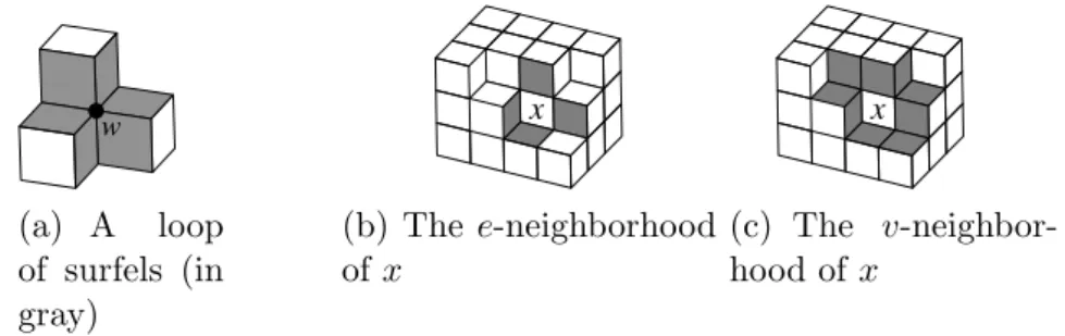
A relation of e−adjacency (see Figure 1(b)) and v−adjacency (Figure 1(c)) can be defined between some surfels that share and edge. Note that the considered adjacency reslation (6, 18) on the set of voxels must be taken into account when defining the e−adjaceny and v−adjacency relations ([8]). In this way, a surfel has exactly 4 e−neighbors, but has a variable number of v−neighbors.
Next, we define a loop in a digital surface Σ as an e-connected component of the set of the surfels of Σ which share a given vertex w. For example, if Σ is the surface of the object depicted in Figure 1(a) (which is made of three voxels), then the vertex w defines two loops: one that contains the six gray surfels, and another one in the back with three surfels. Two voxels are v-adjacent iff they belong to a common loop of Σ.
w (a) A loop of surfels (in gray) x (b) The e-neighborhood of x x (c) The v-neighbor-hood of x
3 On-surface convolution
The work presented in the next sections illustrates the use of on-surface
con-volution, which we introduce here. In the sequel of the paper, Σ is a digital
surface and S is a vector space over R. We define the space of digital surface
filters over Σ as the set of functions from Σ× Σ to R.
Definition 1 (Generalized convolution operator) For f : Σ −→ S and
F : Σ× Σ −→ R, we define the operator Ψ as follows:
Ψf,F : Σ −→ S
x 7−→ ∑
y∈Σ
F (x, y)· f(y)
Intuitively, Ψ acts like a convolution of the values of f on the surface with a convolution kernel whose values should depend on the relative positions of two surfels. We also define the iterated operator Ψ(n).
Definition 2 (Iterated convolution operator) The iterated convolution
operator is defined for n∈ N by:
Ψ(0)f,F = f Ψ(n)f,F = ΨΨ(n−1) f,F ,F if n > 0.
Next, we define an averaging and two derivative filters which we will use in section 4.1 to estimate the normal field on a digital surface.
3.1 The averaging filter
In order to define convolution filters on an arbitrary digital surface, we define some local masks, and then obtain larger masks by iteration. We define a local averaging mask Wavg : Σ×Σ 7→ R. This mask should be seen as a wrapping of
the 2D classical mask (Figure 2(a)) which follows the local shape of the digital surface. The choice of this mask is a heuristics. We tried several masks but this one appears to give particularly good results relating to the Riemannian metrics (see Section 4.2). Intuitively, we define this mask as a generalization of the 2D local mask (and indeed they coincide on a planar surface). The weights are the same as in 2D for the e−neighbors, but for the strict v−neighbors (i.e.
v−neighbord which are not e−neighbors) the weight of what would be a unique
pixel in 2D is split and distributed over the several strict v−neighbors of the loop. The global mass of the mask remains unchanged.
More precisely, let x and y be two surfels of Σ such that y ∈ Nv(x). If y
is v-adjacent but not e-adjacent to x then there is a single loop L of Σ that contains both x and y. In this case, we define δx(y) = card(L)−3. The number δx(y) is used to take into account the number of surfels in a loop containing x which are not e-adjacent or equal to x. Within a loop, all these surfels will
end up with a total contribution of 161.
If there are no such surfels, the weight 1
16 is spread among the two e-neighbors
of x in the loop. Thus, if y is e-adjacent to x, then y has exactly two e-neighbors in Nv(x), say s and t. We define γx(y) as the number of surfels in {s, t} which
are e-adjacent to x.
Now, let x be a surfel of Σ. For any surfel y∈ Σ we define the weight Wavg(x, y) as follows: Wavg(x, y) = 1 4 if y = x, 1 8 + γx(y) 32 if y∈ Ne(x), 1 16·δx(y) if y∈ Nv(x)\ Ne(x), 0 if y /∈ Nv(x).
One can check that for all x∈ Σ, we have∑
y∈Σ
Wavg(x, y) = 1. This may be done
by writing the sum when all the loops that contain x have strict v-neighbors to x, so that γx(y) = 0 for all y ∈ Ne(x). Next, observe that the sum is left
unchanged when one or more loops have only three surfels.
See Figure 2(b) for an example of a v-neighborhood and the associated values of Wavg. 1 1 1 1 2 2 2 2 4 (a) A 2D mask. 2.5 2.5 1 2 2 4 0.5 0.5 0.5 0.5
(b) A surfel x (in gray) and the values of 16 ·
Wavg(x, y) for the surfels
y of Nv(x)∪ {x}. s 0 1 3 2 3 1 E1(s) 2 0
(c) Ordering of vertices and edges for a given surfel s.
Fig. 2. Illustrations of the masks definition.
3.2 The first order derivative filters
We introduce here two directional derivative masks which may be used with the convolution operator to obtain two orthogonal differentiation operators.
as illustrated by Figure 2(c), following the coherent orientation around the outward normal. We denote by Ei(s) the e-neighbor of s that shares with s
its ith edge. Then, we define the derivative masks Du(x, y) and Dv(x, y) for x, y ∈ Σ as follows: Du(x, y) = 1 2 if y = N0(x), −1 2 if y = N2(x), 0 otherwise. Dv(x, y) = 1 2 if y = N1(x), −1 2 if y = N3(x), 0 otherwise.
Given the derivative masks Duand Dv, we may define two derivative operators
Ψf,Du and Ψf,Dv which act on a function f defined on Σ.
4 Normal estimation
In this section, we address the problem of estimating the normal vectors on the surface of a digital object. This estimation is achieved using iterated convolu-tions of the surfel centers with the averaging mask Wavg, followed by a step of
differentiation using the derivative filters Du and Dv defined in section 3.2.
4.1 Surface normal estimation
For different purposes, such as shading methods for visualization or for area estimation, it is interesting to compute normal vectors on the surface of a obtained by digitization of a differentiable surface embedded in R3. In so
doing, our goal is that the computed normals will be as close as possible to the normals on the surface of the underlying differentiable surface. More precisely, the difference between the normals estimated from the digital surface and the normal to the underlying differentiable surface should get smaller when the digitization resolution decreases. Roughly speaking, this property is what is called multigrid convergence in the literature. Several surface normal estimation methods have been proposed, among which we may cite [13,19,11], but no method has been proved to be convergent in that sense so far.
Here, we show that the normal vectors of a digital surface can also be estimated by first averaging the positions of the surfel centers using the iterated convo-lution operator, then computing approximations of two partial derivatives to obtain vectors in the tangent space to the surface, and finally computing a normal vector by a simple cross product of the tangent vectors.
More formally, using the iterated convolution operator Ψ, the averaging mask
for n∈ Z such that Γ(n)(s) is the estimated normal vector of Σ at the center
of s (after n on-surface convolutions). We define the function Γ(n) for n ∈ Z by: Γ(n)(s) = ∆ (n) u (s)∧ ∆(n)v (s) k∆(n) u (s)∧ ∆(n)v (s)k with ∆(n)u = ΨΨ(n) σ,Wavg,Du (resp. for ∆(n)v ) (1)
where ∧ denotes the cross product of two vectors. As the initial averaging process is iterated, the size of the neighborhood taken into account grows accordingly and the precision of the estimate increases as we get closer to the optimal number of iterations. (This number is discussed in section 4.3.)
From the definition of the operator Ψ(n), we see that Γ(n)(s) is the result of a
computation which involves all the surfels of Σ whose distance to s is at most
n in the v-adjacency graph of Σ. In fact, the size of the neighborhood taken
into account when computing Γ(n)(s) grows with n but the weights tend to
follow a geodesic distance which does not coincide with the distance in the
v-adjacency graph. This point, which we claim is a good point, is discussed
in the next section. (The way the weights are distributed when the number of iterations increases is illustrated by Figures 4 and 3(b).) We will present in section 4.3 the results of some experiments.
4.2 Comparison with Papier’s averaging process
In [17,16], Papier et al. define averaging weights on possibly large neigh-borhoods obtained using a breadth-first visiting algorithm of the surfels v-adjacency graph. Their approach generalizes the one of [1] who used only the
e-neighborhood to estimate the normals by averaging the elementary normals
(among the six possible ones). Both methods are based on the averaging of the canonical normals ν(s) of the surfels to estimate the exact normals. This point slightly differs from our method since we are not averaging the normal vectors but simply the surfel centers.
Furthermore, when considering a large neighborhood in an averaging process, one should expect that the mask’s isocurves should be close to the isodistance curves from the center of the mask for the Riemannian metrics of the under-lying differentiable surface. We call this property the Riemannian isotropy of
the mask.
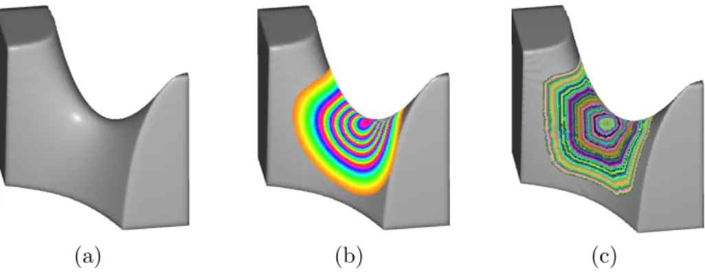
As depicted in Figure 4(a) on a digitized plane with normal vector (1, 1, 1), as well as in Figure 3(c) on a digitized paraboloid, neighborhoods obtained by a breadth-first traversal of the surfels graph do not share the former prop-erty. Therefore, we think that the neighborhoods used by Papier et al. are not optimal when they become large. Our experiments will show that the
neighborhoods should indeed extend when the resolution increases.
(a) (b) (c)
Fig. 3. (a) View of a paraboloid shaded using normals estimated with our method. (b) Response of the iterated averaging filter over the paraboloid compared with a breadth-first traversal (c). (The volume size is 150× 150 × 150 and has 104, 926 surfels.)
In our case, the neighborhood taken into account by the averaging process grows after iterations of convolutions with a local mask, designed to adapt itself to the local geometry of the surface (Section 3.1). Although the actual size of the masks resulting of iterated convolutions also follow the v-adjacency graph, we observe that the weights in these masks have good Riemannian isotropy properties. In order to illustrate how the averaging mask grows, we use a diffusion process: with S =R we choose a surfel s0 ∈ Σ and define the
function δs0 : Σ−→ R such that δs0(s0) = 10
30and δ
s0(s) = 0 for s∈ Σ\{s0}.
Then, we compute Ψ(n)δ
s0,Wavg for a given n. Results of this diffusion process
that we call an impulse response of the averaging filter Ψ(n)f,Wavg are depicted in Figure 4 for the same plane as mentioned previously. Another example is given on the paraboloid depicted in Figure 3(b) with the surfel s0 at the saddle
point, where one can get convinced that the impulse response of our iterated convolution mask behaves as if following a geodesic distance function on the surface.
4.3 Experiments
We have evaluated the precision of the estimation that can be achieved with our method. For this purpose, we have used digitized spheres and tori with several radii and measured the average angular error between the estimated and the exact normal vectors for all surfels. Note that since the estimator relies on an averaging process, we cannot expect it to be precise in the neighborhood of discontinuities of the normal field (edges) or in areas with high curvature. Therefore, it is not suitable for polyhedral shapes, reason why we do not use such shapes in our experiments.
(a) Breadth-first traversal (left) and iterated convolution response (right) over a digitized plane x + y + z = 0.
(b) Plane x + 2y + 3z = 0. (c) Plane 4x + 6.5y + z = 0.
Fig. 4. Breadth-first traversal of the surfels graph (a) and iterated convolution re-sponses (b,c,d).
In the case of 1D functions, a theoretical result is given in [14, Th. 1] which specifies which size should be used for the convolution mask depending on the pixel size or digitization step. The given mask size, or number of convo-lution iterations, guarantees a convergence rate of h23 for the first derivative
estimate, where h is the pixel’s width. However, in our case, no such result has been stated yet. Thus, we address experimentally the problem of finding what convergence speed may be obtained and for which choice of iterations numbers.
In a first series of tests we have measured experimentally the number of con-volution iterations that yield the smallest average angular error in the esti-mation of normal vectors on digitized spheres. The result of this experiment is presented in Figure 5(a). This figure clearly shows an almost linear relation between the radius of the sphere and the optimal number of convolution iter-ations that yield the smallest average angular error of the normal estimation. We thus conjecture that the optimal size for the averaging kernel is in fact linked to the maximal curvature found on the surface.
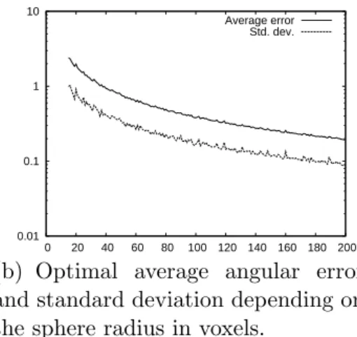
On the other hand, Figure 5(b) shows, on a logarithmic scale, the evolution of the optimal average angular error in degree when the sphere radius increases. As expected, it appears that the method actually achieves a better estimation when the digitization step decreases. This tends to indicate that our estimator is multigrid convergent.
0 20 40 60 80 100 120 140 160 0 20 40 60 80 100 120 140 160 180 200 Optimal iteration number
Linear regression
(a) Optimal number of convolution it-erations depending on the sphere ra-dius in voxels. 0.01 0.1 1 10 0 20 40 60 80 100 120 140 160 180 200 Average error Std. dev.
(b) Optimal average angular error and standard deviation depending on the sphere radius in voxels.
Fig. 5. Normal estimation on digitized spheres.
As a comparison, tests conducted on spheres by Papier in [16] do not clearly show an improvement of the precision when the radius of the sphere increases. Furthermore, they only used umbrellas of order 1 to 5. It is however obvious that the size of the mask should be set according to the resolution, as shown by the measures reported in Figure 5(a). With the approach mentioned in the introduction, the best result given by Lachaud and Vialard in [11] is obtained on a sphere with radius 100 and an average error of 1.51◦ (std. dev. 2.34), when the average error of our method is 0.38◦ (std. dev. 0.17). On a sphere with radius 50, they obtain 2.19◦ (std. dev. 3.46) when we have 0.62◦ (std. dev. 0.26). The earlier paper by Tellier and Debled-Rennesson [19] reports the best average error of 2.84◦ (std. dev. 2.24) for a sphere with radius 25, when our method obtains 1.55◦ (std. dev. 0.71). These results are summarized in Table 1. Figures reported for our method have been obtained using optimal mask sizes.
Radius Papier99 Lachaud03 Tellier99 Our method
θ σ θ σ θ σ θ σ
25 0.96◦ 0.56◦ – – 2.84◦ 2.24◦ 1.55◦ 0.71◦ 50 – – 2.19◦ 3.46◦ – – 0.62◦ 0.26◦ 100 – – 1.51◦ 2.34◦ – – 0.38◦ 0.17◦
Tab. 1. Results comparison with other methods.
However, spheres are not general enough to put to the test a surface normal estimator. This is at least because a sphere has a constant and positive Gaus-sian curvature. Therefore, we have tested our method on several tori with increasing radii, rotated along the three axes. Tori are nice for this test be-cause they have both positive and negative Gaussian curvatures. The results are depicted in Figure 6, where each torus had a small radius of half its large
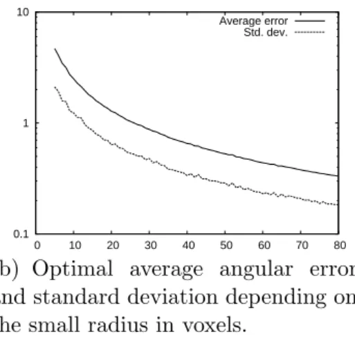
one. Again, the average angular error and its standard deviation decrease with an increasing resolution, as show by Figure 6(b).
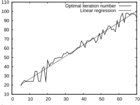
Figure 6(a) still shows a linear dependence between the optimal convolution kernel size and the small radius of the torus. Again, this tends to confirm the link between the optimal size and the maximum curvature which, in the case of a torus, is precisely the inverse of its small radius. Indeed, a change in the ratio between the large and the small radius of the tori has no significant influence on the slope depicted by Figure 6(a). This point has been checked on tori with different ratios: the result is presented in Figure 7(a) which shows that the relation between the optimal number of iterations and the small radius is not altered by a change of the ratio. The same remark does not apply when considering the link with the large radius (Figure 7(b)).
0 10 20 30 40 50 60 70 80 0 10 20 30 40 50 60 70 80 Optimal iteration number
Linear regression
(a) Optimal number of convolution it-erations depending on the small ra-dius in voxels. 0.1 1 10 0 10 20 30 40 50 60 70 80 Average error Std. dev.
(b) Optimal average angular error and standard deviation depending on the small radius in voxels.
Fig. 6. Normal estimation on digitized tori.
0 10 20 30 40 50 60 70 80 90 0 10 20 30 40 50 60 70 80 90 2 2.5 3
(a) Optimal number of iteration ac-cording to the small radius.
0 10 20 30 40 50 60 70 80 90 0 50 100 150 200 250 2 2.5 3
(b) Optimal number of iteration ac-cording to the large radius.
Fig. 7. Optimal number of iterations on tori with different parameters. The ratio between the large and the small radius of each torus is respectively 3, 2.5 and 2.
4.4 Sensitivity to noise
Since our method is based on an averaging process that may be seen as a low-pass filtering, it is expected to be less sensitive to noise than methods based on the recognition of geometric primitives such as digital lines or planes. In order to measure the sensitivity of our estimator, we have repeated the measures of the last section but on noisy objects.
For that purpose, we used digitized spheres and tori on the surface of which
simple voxels have been added or removed. Intuitively, simple voxels are voxels
the removal or addition of which does not change the topology of a discrete object. (See [10,6] for a definition and characterization of simple points in 3D.) A given percentage of the simple voxels are randomly chosen to be removed or added. This percentage will be called here the “noise level” and has been set to 20% in our tests. The noisy counterparts of the sphere and torus of Figure 8(a) are depicted in Figure 8(b). Note that the tori used in our tests do not have a trivial orientation but are rotated along the three coordinate axes.
(a) Digitized sphere and torus (b) Noisy version of the digitized sphere and torus. (Noise level is 20%.)
Fig. 8. Spheres and tori used for the tests.
Results of our experiments are depicted in Figure 9. In Figure 9(a) the optimal number of iterations for the (best) normal estimate is depicted according to the radius of the digitized spheres. The corresponding average and standard deviation of the angular error for each radius is given in Figure 9(b). The same measures on tori are depicted in Figure 10.
In both cases we observe that the average angular error still decreases when the resolution increases, while the standard deviation of the error is almost constant: about 25◦ for the spheres and 10◦ for the tori. A closer look at the angular error distributions shows that they are clearly localized around the mean values but have several outliers which degrade the standard deviations. In fact, outliers come from degenerated surfel centers configurations that ap-pear after smoothing in regions with high curvature, i.e. at the scale of a few voxels. In these regions, the vector products used to compute the estimated normal vectors take into account very small vectors whose directions are not
representative, hence we get a very poor result for the normal. Furthermore, the noise level being a constant percentage of the size of the surface, the amount of degenerated configuration tends to follow the total number of sur-fels, hence we observe the stability of the standard deviation: the more surfels there are, the more outliers there are too.
10 20 30 40 50 60 70 80 90 100 110 0 10 20 30 40 50 60 70 Optimal iteration number
Linear regression
(a) Optimal number of convolution it-erations depending on the sphere ra-dius. 1 10 100 0 10 20 30 40 50 60 70 Average error Std. dev.
(b) Optimal average angular error and standard deviation according to the sphere radius.
Fig. 9. Normal estimation on noisy digitized spheres.
0 50 100 150 200 250 300 0 10 20 30 40 50 60 70 Optimal iteration number
Linear regression
(a) Optimal number of convolution it-erations depending on the small ra-dius. 1 10 100 0 10 20 30 40 50 60 70 Average error Std. dev.
(b) Optimal average angular error and standard deviation according to the small radius.
Fig. 10. Normal estimation on noisy digitized tori. The large radius of the tori is twice the small one.
4.5 Computation times
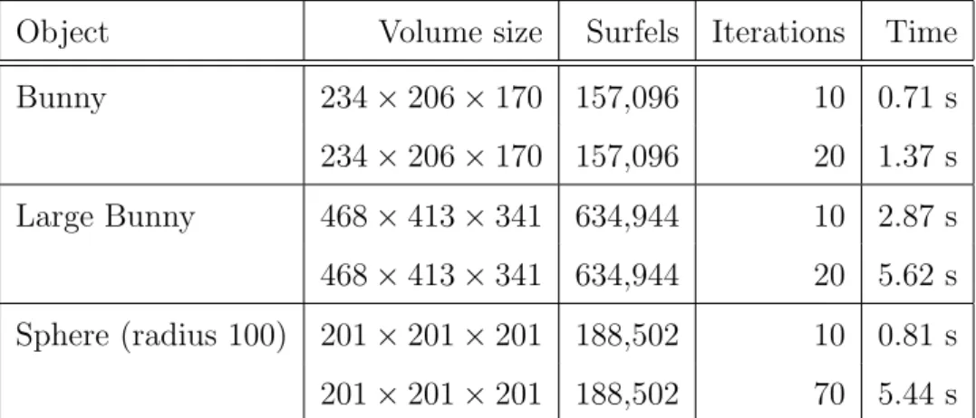
The complexity of our normal estimator is O(m.n) where m is the number of surfels of the surface and n is the number of iterations of the averaging process. In order to give an idea of the effective cost of the method, we provide in Table 2 the computation times obtained with several objects on an Intel Core 2 Duo T5600 processor, 1.83Ghz.
Object Volume size Surfels Iterations Time Bunny 234× 206 × 170 157,096 10 0.71 s 234× 206 × 170 157,096 20 1.37 s Large Bunny 468× 413 × 341 634,944 10 2.87 s 468× 413 × 341 634,944 20 5.62 s Sphere (radius 100) 201× 201 × 201 188,502 10 0.81 s 201× 201 × 201 188,502 70 5.44 s
Tab. 2. Computation times on several objects.
4.6 Surface shading using estimated normals
Precise normal estimates may be used together with a lightening model to render the surface of a 3D volume. In this kind of rendering, only three different primitives are used since at most three kind of surfels are visible depending on the point of view. Such renderings are depicted in Figure 11 where we used our estimated normals (with an arbitrary iteration parameter) to compute the diffuse reflection. A comparison with a rendering found in [11] is given by Figure 12.
(a) The Al volume. Volume size is 150×368×400 and the surface is made of 346,936 surfels.
(b) The Stanford bunny volume. Vol-ume size is 468×413×341 and the sur-face is made of 634,944 surfels. Fig. 11. Surface shading using the normals estimated with our method.
(a) Flat shading. (b) Shading with diffuse reflection according to the normals at surfels estimated with our method.
(c) Shading illustration extracted from [11].
Fig. 12. Surface shading comparison with the normal estimate by Lachaud and Vialard. The sphere has a radius of 30 voxels.
5 Conclusion and perspectives
We have defined an averaging operator based on a convolution over the surface of a digital object, as well as directional derivative operators. When combined, these operators may be used to precisely estimate the normal vectors on the surface of a digitized object as shown by our experiments. The implemen-tation of this method is straightforward (as compared to methods based on arithmetical digital planes recognition of even contruction of a mesh from the digital surface). Although we used floating point arithmetic in our implemen-tation, the averaging filter may be defined using integers-only operations with a delayed normalization step.
We also have estimations of partial differentials, and we can try to estimate higher order partial differntials. Based on this idea, some estimates of Gaussian curvature, mean curvature, and max curvature have been obtained ([7]). This will be tackled in future works.
A link was experimentally established between the maximal curvature on an object and the optimal size of the averaging mask that yield to the best normal estimate. This link should be further investigated. Indeed, no way has been given in this paper to determine the optimal number of iterations for a real-world object.
Finally, a mathemaical proof of multigrid convergence, and eventually a com-plete theory of differential calculus on a digital surface should be the ultimate goal. However, this appears to be a rather difficult task.
References
[1] L.-S. Chen, G. T. Herman, R. A. Reynolds, J. K. Udupa, Surface shading in the cuberille environment, IEEE Journal of computer graphics and Application 5 (12) (1985) 33–43.
[2] D. Coeurjolly, F. Flin, O. Teytaud, L. Tougne, Multigrid convergence and surface area estimation, in: Geometry, Morphology, and Computational Imaging, vol. 2616 of Lecture Notes in Computer Science, Springer, 2003. [3] D. Coeurjolly, R. Klette, A comparative evaluation of length estimators of
digital curves, IEEE Transactions on Pattern Analysis and Machine Intelligence 26 (2) (2004) 252–257.
[4] I. Debled-Rennesson, J.-P. Reveill`es, A linear algorithm for segmentation of digital curves, International Journal of Pattern Recognition and Artificial Intelligence 9 (4) (1995) 635 – 662.
[5] L. Dorst, A. W. Smeulders, Length estimators for digitized contours, Computer Vision, Graphics, and Image Processing 40 (3) (1987) 311–333.
[6] S. Fourey, R. Malgouyres, A concise characterization of 3D simple points, Discrete Applied Mathematics 125 (1) (2003) 59–80.
[7] S. Fourey, R. Malgouyres, Normals and curvature estimation for digital surfaces based on convolutions, in: DGCI, vol. 4992 of Lecture Notes in Computer Science, Springer, 2008.
[8] G. T. Herman, Discrete multidimensional Jordan surfaces, CVGIP: Graphical Models and Image Processing 54 (6) (1992) 507–515.
[9] R. Klette, H. J. Sun, A global surface area estimation algorithm for digital regular solids, Tech. rep., Computer science department of the University of Auckland (Sept. 2000).
[10] T. Y. Kong, A. Rosenfeld, Digital topology: Introduction and survey, Computer Vision, Graphics, and Image Processing 48 (3) (1989) 357–393.
[11] J.-O. Lachaud, A. Vialard, Geometric measures on arbitrary dimensional digital surfaces, in: Discrete Geometry for Computer Imagery, vol. 2886 of Lecture Notes in Computer Science, Springer-Verlag, 2003.
[12] J.-O. Lachaud, A. Vialard, F. de Vieilleville, Fast, accurate and convergent tangent estimation on digital contours, Image and Vision Computing 25 (10) (2007) 1572–1587.
[13] A. Lenoir, R. Malgouyres, M. Revenu, Fast computation of the normal vector field of the surface of a 3-d discrete object, in: DGCI’96: Proceedings of the 6th International Workshop on Discrete Geometry for Computer Imagery, Springer-Verlag, 1996.
[14] R. Malgouyres, F. Brunet, S. Fourey, Binomial convolutions and derivatives estimation from noisy discretizations, in: Discrete Geometry for Computer Imagery, vol. 4992 of Lecture Notes in Computer Science, 2008.
[15] R. Malgouyres, A. Lenoir, Topology preservation within digital surfaces, Graphical Models 62 (2) (2000) 71–84.
[16] L. Papier, Poly´edrisation et visualisation d’objets discrets tridimensionnels, Ph.D. thesis, Universit´e Louis Pasteur, Strasbourg, France, in French (1999). [17] L. Papier, J. Fran¸con, ´Evalutation de la normale au bord d’un objet discret 3D,
Revue de CFAO et d’informatique graphique 13 (1998) 205–226.
[18] I. Sivignon, F. Dupont, J.-M. Chassery, Discrete surfaces segmentation into discrete planes, in: International Workshop on Combinatorial Image Analysis, vol. 3322 of Lecture Notes in Computer Science, Springer, 2004.
[19] P. Tellier, I. Debled-Rennesson, 3D discrete normal vectors, in: Discrete Geometry for Computer Imagery, vol. 1568 of Lecture Notes in Computer Science, Springer-Verlag, 1999.
[20] G. Windreich, N. Kiryati, G. Lohmann, Voxel-based surface area estimation: from theory to practice, Pattern Recognition 36 (11) (2003) 2531–2541.