A latent process model for dementia and psychometric tests.

HAL Id: inserm-00177033

https://www.hal.inserm.fr/inserm-00177033

HAL is a multi-disciplinary open access archive for the deposit and dissemination of sci-entific research documents, whether they are pub-lished or not. The documents may come from

L’archive ouverte pluridisciplinaire HAL, est destinée au dépôt et à la diffusion de documents scientifiques de niveau recherche, publiés ou non, émanant des établissements d’enseignement et de

A latent process model for dementia and psychometric

tests.

Julien Ganiayre, Daniel Commenges, Luc Letenneur

To cite this version:

Julien Ganiayre, Daniel Commenges, Luc Letenneur. A latent process model for dementia and psy-chometric tests.. Lifetime Data Analysis, Springer Verlag, 2008, 14 (2), pp.115-33. �10.1007/s10985-007-9057-x�. �inserm-00177033�

A Latent Process Model for Dementia and

Psychometric Tests

Abstract

We jointly model longitudinal values of a psychometric test and diagnosis of dementia. The model is based on a continuous-time la-tent process representing cognitive ability. The link between the lala-tent process and the observations is modeled in two phases. Intermediate variables are noisy observations of the latent process; scores of the psychometric test and diagnosis of dementia are obtained by catego-rizing these intermediate variables. We propose maximum likelihood inference for this model and we propose algorithms for performing this task. We estimated the parameters of such a model using the data of the five-year follow-up of the PAQUID study. In particular this anal-ysis yielded interesting results about the effect of educational level on both latent cognitive ability and specific performance in the mini men-tal test examination. The predictive ability of the model is illustrated by predicting diagnosis of dementia at the eight-year follow-up of the PAQUID study based on the information from the first five years.

Key words: latent process, Brownian motion, joint model, ordinal data, mul-tivariate data, dementia, Alzheimer’s disease, prediction.

1

HAL author manuscript inserm-00177033, version 1

HAL author manuscript

1

Introduction

Alzheimer’s disease is clinically characterized by a progressive decline of cog-nitive abilities and is the main cause of dementia. The progressive nature of the disease has two important consequences for modeling. First it is not possible to say that the disease starts at a particular moment. Diagnosis is made at the time of the neurologist’s examination but this does not mean that the disease started at this precise moment, nor even at any precise moment before examination. The second consequence is that psychometric tests which measure cognitive abilities can provide important information regarding the progression of a pathological process which may lead to a diag-nosis of Alzheimer’s disease or dementia. It is therefore interesting to devise models which link the two types of information (diagnosis of dementia and psychometric tests) with three main objectives: to better understand this link, to increase the power for detecting risk factors, to predict dementia using previous observations of psychometric test scores.

The problem can be tackled through joint modeling of an event (onset of dementia) and a longitudinal marker (scores of a psychometric test). Joint modeling of CD4 cell counts and onset of AIDS or death has been proposed by Faucett and Thomas (1996) and Wulfsohn and Tsiatis (1997). Concerning dementia a model has been proposed by Jacqmin-Gadda, Commenges and Dartigues (2005), with the specific aim of estimating a change-point in the regime of cognitive decline. Approaches based on a stochastic process frame-work are particularly well suited to grasp the dynamics of diseases. Hender-son, Diggle and Dobson (2000) proposed a model in which a latent process

acts as a time-dependent variable in a proportional hazards model. Other ap-proaches to joint modeling represent the event as the crossing of a barrier by the latent process (Whitmore, Crowder and Lawless, 1998; Lee, DeGruttola and Schoenfeld, 2000). This approach was developed by Hashemi, Jacqmin-Gadda and Commenges (2003) and applied to joint modeling of dementia and a psychometric test: in this model the latent process was interpreted as representing cognitive ability. The present paper proposes an extension of this work with important differences which make the model much more flex-ible, and thus more usable; in particular, for technical reasons, the Hashemi-Jacqmin-Gadda-Commenges model was restricted to linear time-trends for the latent process.

We propose a new model which enables the diagnosis of dementia and scores on a psychometric test to be analyzed together. The model looks particularly non-standard for dementia because we do not model onset of dementia but diagnosis of dementia at the time of visit. This is in fact more realistic (although interval-censoring was treated in the Hashemi-Jacqmin-Gadda-Commenges model) because onset of dementia is an abstraction; cog-nitive decline is in fact most often progressive. Thus our basic model is that a neurologist diagnoses dementia if the subject has a latent process below a certain threshold at the time of visit. As for scores on the psychometric test, we consider a grid of threshold values cm, such that the subject has score m

if his latent process falls between cm and cm+1 at the time of the visit. This

is a refined model compared with previous work, which treats ordinal scores as continuous. With this approach, both diagnosis of dementia and score on the psychometric test are categorized observations of the latent process.

This is reminiscent of probit models for ordinal data (McCullagh and Nelder, 1989; Chib and Greenberg, 1998), but here the underlying latent process al-lows us to capture the dynamics of the phenomenon under study. Our model is in fact slightly more complicated than the above description, as will be described later.

In section 2 we present a general form of the model which could be applied to contexts other than cerebral aging. In section 3 identifiability is studied and the likelihood is derived. In section 4 we describe the specific model used for dementia and the Mini Mental Score Examination: we begin by describing the PAQUID study, a large cohort study on aging which provides the data we used; then we describe the model, present a small simulation and give results, particularly on the predictive ability of the model. We end with a short conclusion.

2

Model and observations

2.1

Outline of the model

We propose a general model for multidimensional longitudinal data based on a latent process. The observation of type k for subject i at time tij will be

denoted Yk

ij (in our application we will use observations of two types: k = 1:

diagnosis of dementia, k = 2: a psychometric test). As in Dunson (2003) we propose a hierarchical structure where the observations Yk

ij are possibly

coarsening transformations of latent variables θk

ij, and these latent variables

are related to common latent elements.

The common latent element in our model is a latent process Λi(t) which

is defined in continuous time (in contrast with Dunson’s model). In our

application it is natural to suppose that, at any time t, not just measurement times, subjects have a certain cognitive ability quantitatively represented by Λi(t) . Our approach allows unequally spaced observations which may

differ from subject to subject. The model for the latent process, driven by a Brownian motion, yields a natural correlation structure for the intermediate latent variables θk

ij, without introducing additional parameters which would

have to be estimated.

Another feature of our model is that it may be non-linear in the parame-ters. In the next section we present the model in its most general form that can be easily treated with our approach because it preserves the normality of the θk

ij. Finally the model is a kind of multivariate probit model (Chib and

Greenberg, 1998): it has a more direct interpretation than assuming that the θk

ij are related to the canonical parameters of a distribution in the

exponen-tial family, and it is related to threshold models already used by Hashemi, Jacqmin-Gadda and Commenges (2003) in this application. Moreover it leads to simpler numerical integrals.

Because of the central role of the latent process in our model, we will start by describing it, explaining afterward how it can be observed by specifying what we call “observation equations”.

2.2

Latent process

For each subject i we introduce Λi = (Λi(t))t≥0, a continuous-time stochastic

latent process; in our application Λi(t) will represent the global cognitive

ability of subject i at time t. This latent process is modeled as a function of

explanatory variables as:

Λi(t) = f (β, xi(t)) + F (γ, zi(t))ai+ Wi(t), (1)

where Wi = (Wi(t))t≥0 is a standard Brownian motion. The q-vector of

random effects ai has a multivariate normal distribution: ai ∼ N (0, A); ai

and Wi are independent and the sets (ai, i = 1, . . . , n) and (Wi, i = 1, . . . , n)

are sets of independent random vectors and processes; the functions f (., .): Rp _{× R}l _{→ R and F (., .): R}p _{× R}l _{→ R}q _{are differentiable and possibly}

non-linear; β and γ are vectors of coefficients (some of which may be in-terpreted as regression coefficients, others of which are used to parameterize the non-linearity) and xi(t) and zi(t) are vectors of time dependent covariates

including t itself.

A linear model for the latent process Λi(t) = xi(t)Tβ + zi(t)Tai + Wi(t),

is a particular case of model (1). Note that in a linear model there is no parameter γ.

In the application we might consider the non-linear model: Λi(t) = β1+

β2xi2 + (β3 + β4xi2)xi1(t)β5 + ai1 + Wi(t), where xi1(t) = t is time itself,

xi2 represents educational level. This model is non-linear in both time and

the parameter β5. Introducing this parameter provides more flexibility in

modeling changes over time.

2.3

Observation equations.

We consider that the values of “tests” at different time points are indirect observations of the latent process; in our application the “tests” include both psychometric tests and diagnosis of dementia. We model the link between the latent process and the tests in two phases: first we introduce, for subject

i, intermediate random variables θk

ij which can be seen as potential

mea-surements for each test k = 1, . . . , K of Λi(tij); secondly we represent the

values of the tests as functions of these intermediate variables. The reason for differentiating these two phases is that the θk

ij are linear in Λi(tij) and

have normal distributions while the test functions may be non-linear and discontinuous. The times tij will be treated as deterministic. They might be

random but under the condition that the mechanism leading to incomplete data is ignorable, a condition under which the likelihood treating these times as fixed leads to the same inference as the correct likelihood. We make the same assumption for possibly missing data.

2.3.1 Definition of θk ij.

The intermediate variables for subject i and for test k are defined as: θijk = Λi(tij) + gk(βk, xki(tij)) + Gk(γk, zik(tij))dki + ²

k

ij, (2)

for j = 1, . . . , ni, where gk(., .) and Gk(., .) are analogous to f (., .) and F (., .)

in the definition of the latent process but are specific to the kth _{test; d}k i is

a rk-random vector with normal distribution: dki ∼ N (0, Dk); the

measure-ment errors ²k

ij are identically independently distributed (i.i.d) variables with

normal distributions: ²k

ij ∼ N (0, σ²2k), for all j. The triple (Λi(tij), dki, ²kij) is

a set of independent variables for any choice of i, j, k. A linear model for the intermediate variables θk

ij = Λi(tij) + xki(tij)Tβk+

zk

i(tij)Tdki + ²kij is a particular case of model (2).

2.3.2 Link between θk

ij and the data: the test functions

For subject i, we denote Yk

ij the random variable representing the observation

of the kth _{test on the occasion of the j}th _{visit at time t}

ij. We will consider

the cases of ordinal (including binary) longitudinal data. We consider a test k for which Mkordered values are possible (m ∈ [0, Mk− 1]). Observation of

Yk

ij = m provides the information that θijk lies between two thresholds, that is,

Yk

ij = m if and only if ckm ≤ θkij < ckm+1, with c0 = −∞ and cMk = +∞. The

test function (which is the function of θk

ij that equals Yijk) is in this case a step

function. The cut-off points ck

m are not known and must be parameterized or

estimated directly according to the number of possible values Mk. Generally

we shall represent ck

m as a function of parameters ηk, the dimension of which

may be less than Mk − 1 in order to obtain a more parsimonious model:

ck

m = τk(m, ηk), ∀m ∈ [1, Mk− 1], where τk(.; ηk) is a monotone function.

Binary data are simply a special case of ordinal data for which we only need one cut-off point, ηk

0 for instance. For a binary test, Yijk= 1{θk ij≥η

k 0}.

3

Likelihood Inference

To establish the likelihood we will first study the distribution of the interme-diate variables. Then we establish the likelihood for the case where the tests are ordinal variables as in our application.

3.1

Joint distribution of the intermediate variables

We shall study the distribution of the Kni vector Θi = (θkij; k = 1 . . . , K; j =

1, . . . , ni). It is to be noted that in equations (1) and (2) linearity in the

random effects is assumed: this requirement is important to remain in a

Gaussian framework; that is to say Θi ∼ N (µi, Σi). Thus computing the

distribution of Θi comes down to computing its mean vector µi and variance

covariance matrix Σi. The expectation can easily be computed since we have:

E(θk

ij) = f (β, xi(tij)) + gk(βk, xki(tij))

The variance of Θi is the sum of the variance coming from the latent

process Σi,Λ, the variance of the test specific random effects Σid and the

variance of the noise term Σiε:

Σi = ΣiΛ+Σid+Σiε=    Σ0 iΛ . . . Σ0iΛ ... ... ... Σ0 iΛ . . . Σ0iΛ   +    Σid1 0 0 0 . .. 0 0 0 ΣidK   +    σ2 ε1I_ni 0 0 0 . .. 0 0 0 σ2 εKIni   , where Σ0

iΛ = FiT A Fi+ Γi, and Γi is the covariance matrix associated with

the Brownian motion:

Γi =      ti1 ti1 . . . ti1 ti1 ti2 . . . ti2 ... ... ... ti1 ti2 tini      ,

and Fi =¡F (β, zi(ti1)), . . . , F (β, zi(tini))¢, a q × ni-matrix, and where Σ

k id= Gk i T Dk _Gk i, with Gki =¡Gk(γk, zik(ti1)), . . . , Gk(γk, zik(tini))¢, a rk× ni ma-trix.

3.2

Identifiability

Clearly there must be some constraints on the parameters to ensure identi-fiability. A thorough analysis is beyond the scope of this paper, but we give some insight. We can distinguish three sets of parameters: β = (β, βk_{, k =}

1, . . . , K), γ = (γ, A, γk_{, D}k_{, σ}2

k, k = 1, . . . , K) and η = (ηk, k = 1 . . . , , K)

and the whole set of parameters is α = (β, γ, η). We consider the case of the linear model for the sake of simplicity; in the linear model there is no param-eter γ nor γk_{. Clearly in order that β and γ be identifiable from observation}

of the Yk

ij they should be identifiable from the observation of θkij.

Let us now look at sufficient conditions for this. In the linear model there is a matrix A such that E(Θ) = Aβ. A necessary and sufficient condition for identifiability of β is r(A) = dim(β), where r(A) is the rank of A: this happens if and only if the columns of A are linearly independent. A necessary condition for that is KP ni ≥ dim(β). A sufficient condition of

identifiability of β is:

C1: (i) there is no collinearity of the explanatory variables ; (ii) there are no explanatory variables for one of the equations of the intermediate variable. Point (i) is common in all linear models. That C1 is sufficient for identi-fiability of β can be seen from the structure of the A matrix.

Similarly for the identifiability of γ we consider the condition:

C2: (i) There is no random effect for one of the equations of the inter-mediate variable; (ii) all the matrices FiFiT are not equal.

For instance if there is no random effect for test k we have: varγ(θk i) =

FT

i AFi+ Γi+ σεkI_n

i. If there was non-identifiability there would exist γ

′ _{6= γ}

such that varγ′(θ_ijk) = varγ(θ_ijk), which would entail: F_iT(A′− A)F_i = (σ′

εk−

σεk)I_n

i. However the rank of the left-hand side is q while the rank of the

right-hand side matrix is ni. So unless ni = q for all i, this equality holds

only if A′ _{= A and σ}′

εk = σεk. If n_i = q for all i, we could solve the equation

to find (A′ _{− A) as a function of F}

i leading to the additional requirement

that FiFiT be the same for all i.

As for the identifiability of the whole set of parameters from the observa-tion of the Yk

ij it is difficult to prove a sufficient condition. There is at least

an obvious non-identifiability case that can be detected, and thus avoided. For fixed γ the distribution of the Yk

ij depends only on the ckl − Eβ(θijk) for

l = 1, . . . , Mk−1, k = 1, . . . , K. If the model for the cut-off points makes

it possible to find η′k _{such that: c}k

l(η′k) = ckl(ηk) + ∆ for l = 1, . . . , Mk−1,

k = 1, . . . , K and if there is an intercept (β1) in the equation of the latent

process, then the distribution of the Yk

ij specified by α′, where α′ is defined

by η′_{, β}′

1 = β1+ ∆ and the other parameters equal to those of α, is the same

as that specified by α. To avoid this non-identifiability case we may for in-stance give a fixed value to one cut-off value or the intercept β1, a condition

we call “C3”.

In practice we recommend that conditions C1, C2 and C3 be applied, or analogous conditions since these are particular cases of constraints that may be put on the three levels of the model.

3.3

Likelihood

We will first establish the individual contribution to the likelihood Li(α).

for any subject i. We denote by yk

ij the (realized) observation relative to the

kth _{test on the occasion of the j}th _{visit at time t}

ij, a realization of Yijk. Li is

the probability according to the model of the observed trajectory, that is: Li(α) = P [Yi11 = y1i1, . . . , Yin1i = y 1 ini, . . . , Y K i1 = yKi1, . . . , YinKi = y K ini]

We will now define the sets over which integration will be required. Let

Ck

ij be the interval relative to observation yijk and intermediate variable θkij.

Cijk = [c k yk ij, c k yk ij+1]

If we define Ci the orthant concerning subject i, Ci = ni,K

⊗

j=1,k=1C k ij, we

obtain for the entire path concerning subject i Li(α) = P [Yijk = y

k

ij, j = 1, . . . , ni; k = 1, . . . , K] = P [Θi ∈ Ci]

As Θi ∼ N (µi, Σi), we just need to integrate the multivariate normal

probability density function φ(µi,Σi) over the Ci sets:

Li(α) = Z · · · Z Ci φ(µi,Σi)(u)du.

Missing values cause no problem because if value at test k at time tij is

missing, the integration set Ck

ij for this observation becomes ] − ∞, +∞[, so

this simply decreases the multiplicity of the integral by one. It is possible to include a truncation condition by writing a conditional likelihood. See the ap-plication section (4.3) for an illustration. Independence over subjects makes it possible to obtain the likelihood of the sample as L(α) =Qn

i=1Li(α).

3.4

Maximization algorithm

The likelihood is difficult to compute since each Li involves a multiple

in-tegral, which has to be computed numerically (see Evans and Swartz, 2000, for a review). However, an advantage of our model is that the integrals that we have to compute are integrals of normal multivariate densities. Efficient techniques exist for this task: in particular the algorithms proposed by Genz (1992) allow us to compute such integrals up to a multiplicity of 20. The

multiplicity of the integral for computing Li is Kni. For instance in our

application we have K = 2 and ni = 4, which leads to a multiplicity of 8, a

feasible problem with the Genz algorithm.

Maximum likelihood estimators can be obtained by using quasi-Newton algorithms. We have considered a Marquardt algorithm (Marquardt, 1963) and an algorithm used by Heddeker and Gibbons (1994) and Todem, Kim and Lesaffre (2007), in which the Hessian of the log-likelihood is replaced by the estimated variance matrix of the score. This algorithm has been further stud-ied and called “Robust-variance scoring” (RVS) algorithm by Commenges et al. ( arXiv:math.ST/0610402, http://arxiv.org/abs/math/0610402). An ad-vantage of the RVS algorithm is that it needs only first derivatives of the log-likelihood, and the standard errors are obtained from the estimated vari-ance matrix of the score at the maximum. Our experience shows that the RVS algorithm is more than twice as fast as the Marquardt algorithm in our problem.

4

Application

4.1

The PAQUID study and the studied sample

The proposed approach was applied to the joint modeling of diagnosis of de-mentia and a psychometric test, the Mini Mental State Examination (MMSE) (Folstein et al. 1975), using the data of the PAQUID cohort.

The PAQUID program on cerebral aging is based on a large cohort ran-domly selected in a population of subjects aged 65 years or older, living at home in two administrative areas of southwest France (Gironde and Dor-dogne). Our analysis bears on the first eight years of the follow-up of this

study. In addition to the initial visit, subjects were seen approximately after one, three, five and eight years in Gironde and after three, five and eight years in Dordogne; the successive visits are denoted by T0, T1, T3, T5 and T8. At each visit the MMSE was measured and diagnosis of dementia was made by neurologists, based on the DSMIII-R criteria (for details see Leten-neur et al., 1999). We will use the first five years to fit the model and the eight-year follow-up to assess the predictive ability of our model.

Our sample was composed only of women who were not demented at the initial visit. It is safer to analyze men and women separately because the dynamics of aging seems to be quite different between the genders (see Commenges et al., 2004). Because there are more women than men in the PAQUID sample we chose to focus on women. We introduced the condition of being non-demented at the initial visit because it is doubtful that the PAQUID sample is representative of the whole population (demented and non-demented): demented subjects are often institutionalized. The condi-tion of being non-demented at entrance must be taken into account in the likelihood (see section 4.3). At the initial visit there were five cases which, although not diagnosed as demented, obtained a MMSE score of zero (this can be seen in Figure 1): these subjects had cognitive impairment due to causes other than dementia (stroke, psychiatric illness); we have chosen to keep them in the sample.

We thought that the evolution of cognitive ability may be strongly af-fected by dementia and it was not our aim to describe this evolution; in consequence, further observations of the MMSE after diagnosis of dementia were not taken into account. This artificial right-censoring is ignorable: the

reason is that it is done on the basis of an observed variable included in the model and this can be proved using results of Commenges and G´egout-Petit (2005).

Finally, our study sample was composed of 2131 women aged 65 years or older and who were not demented at the initial visit. During the 5-year follow-up we had 5622 observations of the MMSE. We had also 5742 assessments of the demented status; among them, 126 were diagnoses of dementia.

4.2

The model applied to the PAQUID sample

4.2.1 The explanatory variables

The different components of the model we developed may depend on educa-tional level and a variable indicating whether the test was administered for the first time (to take into account a possible practice effect): educational level has been shown to be a risk factor of dementia (Letenneur et al., 1999) and a practice effect of the MMSE has been found (Jacqmin-Gadda et al., 1997). Moreover, there has been debate about the necessity of correcting the MMSE for educational level in order to determine cognitive impairment, a prognostic factor of dementia.

The most difficult problem is to define what time is in our model. Since we wish to relate cognitive decline to age it is natural to determine a time-scale for each subject closely related to age. We could consider that the time that is relevant for a subject is the time elapsed since her birth, that is, age. However, in this model we do not wish to model the evolution of cognitive ability from birth (we would have to develop a much more complicated model)

but only the decline of cognitive ability from an age at which we think that this phenomenon may start for a non-negligible fraction of the population. We took as origin the age of 65 for the two following reasons: (i) we have observations from age 65, making it awkward to take a later origin, which would lead to negative times: particularly in a non-stationary (due to the Brownian motion) and non-time-homogeneous (due to the non-linearity in t) model this would not make sense; (ii) we have tried earlier time origins but this yielded lower likelihoods.

Educational level is represented by the binary variable that we will denote by Edi so that Edi = 1 if subject i has obtained a primary school diploma

and 0 if not. Practice effect, denoted by Prai, is defined as: Prai(t) = 1 for

t ≤ ti1 and Prai(t) = 0 for t > ti1.

For clarity of interpretation we will describe the model directly in terms of t, Edi and Prai(t) rather than using the general notations.

4.2.2 The latent process

In this application of our model, the latent process represents cognitive abil-ity: diagnosis of dementia and MMSE will be considered as indirect mea-surements of this. The latent process is defined by equation (1) in which we specify f (., .) as:

f (β, xi(t)) = (β1+ β2Edi) + (β3+ β4Edi)tβ5.

As for the function F (., .) we tried: F (γ, zi(t))ai = ¡1, tγ1

¢µ a1,i

a2,i

¶

= a1,i + a2,itγ1. It was natural to assume

γ1 = β5, that is, there is a vector of random effects ai of size q = 2 bearing on

the intercept β1 and the slope β3. However the algorithm failed to converge

when we tried to estimate the two variance parameters and the correlation coefficient of the two random effects, probably due to the presence of the Brownian motion. The algorithm converged if we assumed a diagonal vari-ance matrix for ai: A = µσ

2

a1 0

0 σ2 a2

¶

. We also tried a simpler model with only one random effect obtained with the F (γ, zi(t))ai = ai; since this simpler

model gave nearly the same result, we present this simpler model hereafter. For this model the latent process is defined as:

Λi(t) = (β1+ β2Edi) + (β3+ β4Edi)tβ5 + a1,i+ Wi(t). (3)

4.2.3 Observation equations.

In this application, we jointly model the diagnosis of dementia and the MMSE score, so that K = 2: the first “test” (k=1) is diagnosis of dementia and this is a binary variable; the second “test” (k=2) is the MMSE which has 31 values. The specification of the equations for the intermediary variables is guided by interpretability and identifiability issues.

We have introduced a random effect in the model of the intermediate variable θ1

ij for diagnosis (k = 1). In formula (2) we took g1i(β1, x1i(tij)) = 0

and G1

i(γ1, z1i(tij)) = 1; there was one random effect d1i ∼ N (0, σd21). This

random effect makes it possible that subjects with a low latent process are not diagnosed as demented; this may happen because some subjects have always had low cognitive ability not linked to a neurodegenerative process. We did not introduce additional error term, that is to say σ2

ε1 = 0, nor explanatory

variables (thus satisfying condition C1 in section 3.2). Thus the intermediate variable for dementia is:

θij1 = Λi(tij) + d1i. (4)

To relate this variable to the diagnosis of dementia (which means defining the “test function”) we just need one cut-off value given by the parameter η0: Yij1 = 1 if and only if θ1ij ≤ η0. Our notation here for the parameters η

differs slightly from the general case: we use η0 for dementia and η1, η2 and

η3 for the MMSE, the meaning of which is explained below.

As for the MMSE (k = 2) we took into account both the practice effect and the specific impact of educational level on MMSE. The practice effect is only located on the first visit (j = 1) and we introduced an interaction with educational level (meaning that the practice effect may not be the same for subjects with or without a primary school diploma). Thus in formula (2) we took g2

i(β, xi(tij)) = β12Edi + β22Prai(tij) + β23Edi × Prai(tij). No specific

random effect was introduced in the MMSE equation (condition C2), so G2

i(γ2, xi(tij)) = 0. There was, however, an error term of variance σε22. Thus,

the intermediate variable for MMSE was:

θ2ij = Λi(tij) + β12Edi+ β22Prai(tij) + β32Edi× Prai(tij) + ε2ij. (5)

MMSE takes values between 0 and 30, so we have M2 = 31. It is judicious

to use a model for the family of cut-off points c2

m = τ2(m, η) which is more

parsimonious than considering all the cut-off values as parameters. We have c2

M2 = +∞ and c

2

0 = −∞ and for satisfying condition C3 we fixed c2M2−1

arbitrarily at the value c2

M2−1 = 40. There is no reason that the MMSE scale

be linear with respect to the latent process scale so we used the following model yielding unequally spaced cut-off points: c2

m = 40 − η1(M2− 1 − m)η

2.

We limited this power model to m ∈ [1, M2− 3] and we gave an independent

parameter η3 for c2M2−2, which made it possible to improve the fit as compared

to extending the above model up to M2 − 2. Thus our model for the test

function for MMSE involves three parameters: η1, η2 and η3.

4.3

The likelihood for the application

We computed the likelihood according to section 2. We also had to include the selection condition mentioned in section 4.1: since only non-demented subjects were included, the likelihood is conditional on {θ1i1 > η0} (the event

that subject i is not diagnosed as demented at initial visit ti1); the conditional

likelihood for subject i is Li/P (θi11 > η0). We obtain from the model: θi11 ∼

N ¡ f (β, xi(ti1)) , Σi(1, 1) ¢, so that we have: P (θ1_i1 > η0) = Φ ³f (β, x_i(t_i1)) − η₀ q σ2 a1 + ti1 + σ 2 d1 ´ .

The likelihood was maximized using the RVS algorithm described in sec-tion 3.3.

4.4

A Simulation

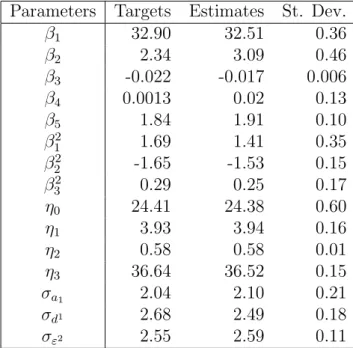
In order to demonstrate the ability of our algorithm to maximize such a complex likelihood we tried it on a simulated data set. We generated a sample of size n = 2131 with the same age distribution at the initial visit and the same proportion of educated and non-educated subjects as in the real data sample from the PAQUID study. We generated 4 visits as in the real data set, the initial visit and visits after one, three and five years. The values of the 16 parameters were taken equal to the values estimated in the real data set. We took as starting values: β2 = β3 = β4 = β12 = β22 = β32 = 0; β1 = 38.5; β5 = 1;

η0 = 30; η1 = η2 = 1; η3 = 39; σa1 = 10

−5_{; σ}

d1 = σ_ε2 = 10. The algorithm

converged in 19 iterations. The results are given in Table 1. We see that the estimated values are reasonably close to the target values and that the .95 confidence intervals include these values. The algorithm converged toward the same point from different starting values. We also verified the quality of the inverse Hessian for giving estimates of the variances of the estimators of the parameters by checking a reasonable agreement between some Wald tests and likelihood ratio tests. On the whole, the algorithm seems to be reliable.

4.5

Model estimated from the PAQUID data

The values of the parameters estimated from the PAQUID sample are shown in Table 2. As expected there is a significant mean trend of decrease of global cognitive ability (see β3) with a shape not far from a quadratic form

(see β5). There is a significant heterogeneity around the intercept (see σa1).

The significant random effect for dementia (σd1) means that some subjects

are not diagnosed demented at repeated visits in spite of low cognitive ability. The value of 0.58 for parameter η2 indicates that a difference of one

point of MMSE corresponds to a larger difference in cognitive ability for high cognitive level than for a low one; in other words, the sensitivity of MMSE is better for low levels than for high levels; this is graphically illustrated in Figure 2 which displays a grid of the cut-off values making it clear that a larger difference in latent process (or rather intermediate variable) values is necessary to make one point of difference for the MMSE for higher rather than for lower levels. This is reminiscent of the mixed linear model applied by Jacqmin-Gadda et al. (1997) to the square-root of 30 minus MMSE (in fact the number of errors).

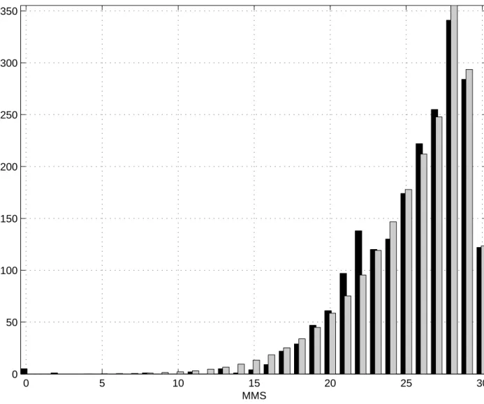
In order to assess the degree of realism of our model for the MMSE we computed the expected numbers of subjects having score m at the MMSE at T0: this was achieved by computing for each subject the probability of having score m and summing the 2131 probabilities. The computation of these probabilities was carried out with the estimated model, taking into account the ages, educational levels and the practice effect, as well as the different variability terms and the use of formulas similar to that used for the prediction in section 4.6. Figure 1 compares the histograms of observed MMSE scores with the histogram of expected numbers; it can be seen that they are quite similar. There is a slight discrepancy at scores 22 and 21: this artefact is due to the screening design for diagnosing dementia in the PAQUID study at T0 which used the threshold 24 and which probably led interviewers to put 22 or 21 rather than 24 for some subjects (to trigger the visit of a neurologist).

We can make an approximate link between the threshold for dementia η0 and values at the MMSE. Taking zero values for the random effect for

dementia and errors for the MMSE, the value of the threshold approximately corresponds to MMSE= 19 and MMSE= 21 for low and high educational levels respectively. (The value 19 is found as follows. For a subject with a low educational level we have from (6): θij2 = Λi(tij) and E(θij1) = Λi(tij);

thus if we consider subjects for which E(θ1

ij) = η0 they have θ2ij = η0; the

corresponding value m0 of the MMSE score satisfies the equation η0 = 40 −

η1(30 − m0)η2).

Our model allows us to distinguish the effect of educational level on the latent cognitive ability on the one hand and on the MMSE score on the other.

Educational level has a significant effect (β2) on the intercept of the cognitive

ability process, but not on the slope (β4); there is a highly significant effect

of educational level (β2

1) for the MMSE. To sum up, (because of the positive

β2

2) subjects with a high educational level tend to have a higher MMSE than

subjects with a low educational level, for the same value of the latent process (true cognitive ability), leading to a diagnosis of the former as demented at higher MMSE levels than the latter; on the other hand (because of the positive β2) subjects with a high educational level tend to have a higher value

of the latent process than subjects with a low educational level, leading to a lower rate of diagnosis of dementia for the former as compared to the latter. Finally, there is a significant effect of practice effect (β2

2)(subjects have a

lower MMSE at the first visit than expected); the interaction of practice with educational level (β2

3) is not significant.

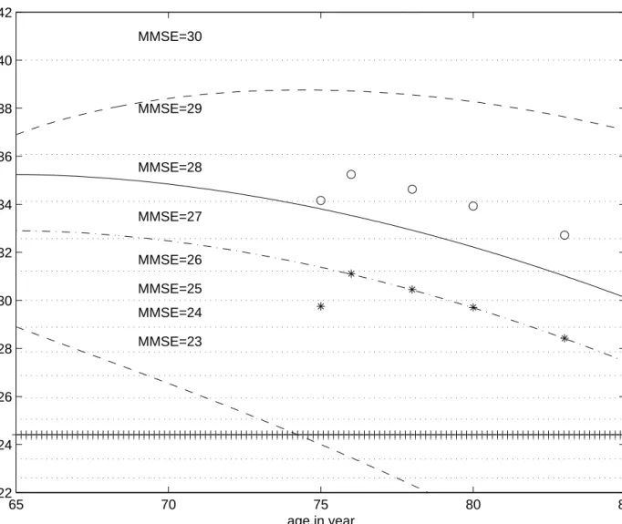
Several features of these results can be best illustrated by a graph. Figure 2 shows, in the latent process scale, both the grid of the cut-off values for the MMSE (horizontal dotted lines) and the threshold for diagnosis of dementia (the horizontal crosses line at η0 = 24.41). It also shows the expected value

of the latent process of cognitive ability for subjects with a low and a high educational level (the curve for low educational level starts at the value of the intercept β1 = 32.90). The curves are approximately parallel and the

curve for low educational level below; this explains that a larger incidence of dementia has been observed in this group (Letenneur et al., 1999). We can see that the decline of this expected value is very slow near the age of 65 and accelerates for older ages for both low and high educational levels. This is rather in agreement with normative values which have been established in the

United States (Crum et al., 1993) and in France (Lechevallier-Michel et al., 2004) although the results can not be compared directly: one main difference is that normative values exclude demented subjects; another difference is that we model the practice effect. Figure 2 also shows the dispersion for the values of the latent process by showing a region in which 95% of the values for low educated subjects lie at each age. The lowest bound curve (dashed line) crosses the threshold value (around 75) and so, it is graphically apparent that a growing number will be diagnosed as demented with older age.

Moreover Figure 2 illustrates the effect of educational level on values of the MMSE (for a given value of the latent process), as well as the practice ef-fect on MMSE scores. It shows the expected values of intermediate variables for MMSE (θ2

ij) for subjects with low and high educational levels entering

at 75 in the study and seen one, three, five and eight years after. In our model these expected values are equal to the expected value of the latent process for subjects with a low educational level (the stars) except for the first visit where the value is lower due to the practice effect: this is because if Edi = 0 and Prai = 0 we have from formula (5) θ2ij = Λi(tij) + ε2ij, so

that E(θ2

ij) = E[Λi(tij)]. As already mentioned, there is a grid indicating the

values of the MMSE obtained as a function of the intermediate variable. For instance a subject with a low educational level who has her intermediate vari-ables equal to the expectations and entering at 75 at T0 would have MMSE values 24, 25, 25, 24 and 23 at T0, T1, T3, T5 and T8 respectively. The ex-pectations of the intermediate variables for subjects with a high educational level are higher than the expected value of the latent process for the same time. The results illustrated in this figure, contribute to the debate

ing the possible correction of the MMSE to take the educational level into account and regarding the effect of educational level on dementia. It appears that educational level has an effect on global cognitive ability (our latent process), and thus on dementia, but also has a specific effect on MMSE.

4.6

Prediction of dementia diagnosis

The model may be used for predicting diagnosis of dementia for subject i at time ti,ni+1, given the MMSE values at the successive visits (1, . . . , ni) and

given that subject i has not been diagnosed as demented up to visit ni. The

information that we have up to visit ni is summarized by the event Θi ∈ Ci.

The probability that subject i is diagnosed as demented at ti,ni+1 is

pi = P [θi,n1 i+1 ≤ η0|Θi ∈ Ci] =

P [(θ1

i,ni+1 ≤ η0) ∩ (Θi ∈ Ci)]

P [Θi ∈ Ci]

.

This expression is not affected by the condition of not being diagnosed as demented up to visit ni as the corrective conditional probability cancels out

in the ratio. In order to compute the numerator we need the joint distribution of θ1

i,ni+1 and Θi. This is a normal distribution with expectation:

µ∗_i = µ µi E[θ1 i,ni+1] ¶ = µ µi f (β, xi(ti,ni+1)) ¶ , and variance matrix Σ∗

i formed by the block Σi augmented by the correlation

between θ1

i,ni+1 and Θi and the variance of θ

1

i,ni+1. These are given by:

cov(θi,n1 i+1, θ

1

ij) = σ2a1 + tij + σ

2

d, for j = 1, . . . , ni+ 1;

cov(θ1_i,ni+1, θ_ij2) = σ2_a1 + tij, for j = 1, . . . , ni.

We selected subjects who had not been diagnosed as demented up to visit T5 and who had been seen at T8: N = 1187 subjects satisfied these

criteria. We computed their individual probabilities pi of being diagnosed

demented at visit T8, using the values of the parameters θ estimated from the follow-up up to five years. One aim was to predict the number Nd of

subjects diagnosed as demented at T8: a natural predictor is the expectation of Nd (conditional on information up to T5) which is

PN

i=1pi. We found

ˆ

Nd = 46.6. A predictive interval can be computed using the fact that varNd=

PN

i=1pi(1 − pi) and treating Nd as approximately normal; we found that the

95% predictive interval was [34.1; 59.2]. We observed 56 new diagnoses at T8, a number inside the predictive interval.

Another way to assess the predictive ability of our model for diagnosis of dementia at T8 was to consider the pi’s as quantitative values on which

a classification as positive or negative could be made according to a cut-off value, as in the theory of diagnostic tests. Sensitivity and specificity can be computed for each cut-off value and the ROC curve relates sensitivities and specificities for the different cut-off values. Figure 3 gives the ROC curve for our prediction of dementia diagnosis. In particular, the area under the ROC curve is a summary measure of performance of the test. The area under the ROC curve of our model is 0.82, a rather good value.

5

Conclusion

We have developed a general model for multivariate longitudinal ordinal data. The reviewers insisted on the need for a thorough study of identifiability in this model. Such a study is challenging: we have given reasonable condi-tions to avoid unidentifiability, which are satisfied by the model used in the application. Moreover the simulation study shows that in the region of the

parameter space considered there is practical identifiability for the model used.

The model could be easily extended to include continuous data: we could use for test k a continuous function hk(.) : Yijk = hk(θkij). Such a test function

could be chosen in a family of functions depending on a parameter ηk_{. For}

instance Proust et al. (2006) in an analogous problem have chosen the family of beta cumulative distribution functions indexed by two parameters.

When modeling cerebral aging one would also have to model death: joint modeling of dementia and death has been achieved by the use of an illness-death model (Joly et al., 2002; Commenges et al., 2004) but cognitive ability was not modeled. It is not possible to rigorously treat the joint occurrence of diagnosis of dementia, psychometric tests and death with existing mod-els. However, approximate inference can be made by considering death as censoring, as has been done in this paper.

Our model is useful for jointly modeling psychometric tests and diagnosis of dementia but could be applied to other epidemiological contexts.

References

Chib S, Greenberg E (1998) Analysis of multivariate probit models. Biometrika, 85:347-361.

Commenges D, G´egout-Petit A (2005) Likelihood inference for incompletely

ob-served stochastic processes: general ignorability conditions. arXiv:math.ST/0507151, http://arxiv.org/abs/math/0507151.

Commenges D, Joly P, Letenneur L, Dartigues JF (2004) Incidence and prevalence of Alzheimer’s disease or dementia using an Illness-death model. Stat Med 23:199-210.

Crum RM, Anthony JC, Bassett SS, Folstein MF (1993) Population-based norms for the mini-mental state examination by age and educational level, JAMA, 18:2386-2391.

Dunson DB (2003) Dynamic latent trait models for multidimensional longitudinal data. J Am Stat Assoc, 98:555-563.

Evans M, Swartz T (2000) Approximating integrals via Monte Carlo and deter-ministic methods. Oxford University Press; Oxford.

Faucett CL, Thomas DC (1996) Simultaneously modeling censored survival data and repeatedly measured covariates: a Gibbs sampling approach. Stat Med 15:1663-1685.

Folstein MF, Folstein SE, McHugh PR (1975) Mini-Mental State. A practical method for grading the cognitive state of patients for the clinician. J Psych Res 12:189-98.

Genz A (1992) Numerical computation of the multivariate normal probabilities. J Comput Graph Stat 1: 141-150.

Hashemi R, Jacqmin-Gadda H, Commenges D (2003) A latent process model for joint modeling of events and marker. Lifetime Data Anal 9: 331-343. Hedeker D, Gibbons R (1994) A random-effects ordinal regression model for

mul-tilevel analysis. Biometrics 50: 933944.

Henderson R, Diggle P, Dobson A (2000) Joint modeling of longitudinal measure-ments and event time data. Biostatistics 1: 465-480.

Jacqmin-Gadda H, Commenges D, Dartigues JF (2006) Random changepoint model for joint modeling of cognitive decline and dementia, Biometrics, 62:254-260.

Jacqmin-Gadda H, Fabrigoule C, Commenges D, Dartigues JF (1997) A 5-year longitudinal study of the mini-mental state examination in normal aging. Am J Epidemiol 145:498-506.

Joly P, Commenges D, Helmer C, Letenneur L (2002) A penalized likelihood approach for an illness-death model with interval-censored data: application to age-specific incidence of dementia. Biostatistics 3:433-443.

Lechevallier-Michel N, Fabrigoule C, Lafont S, Letenneur L, Dartigues JF (2004) Normative data for the MMSE, the Benton visual retention test, the Isaacs’s set test, the digit symbol substitution test and the Zazzo’s cancellation task in subjects over the age 70: results from the PAQUID Study Revue de Neurologie 160:1059-1070.

Lee MLT, Degruttola V, Schoenfeld D (2000) A model for markers and latent health status. J Roy Stat Soc B 62:747-762.

Letenneur L, Gilleron V, Commenges D,Helmer C, Orgogozo JM, Dartigues JF (1999) Are sex and educational level independent predictors of dementia and Alzheimer’s disease? Incidence data from the PAQUID project. Journal of Neurology Neurosurgery and Psychiatry 6:177-183.

Marquardt D (1963) An algorithm for least-squares estimation of nonlinear pa-rameters. SIAM J Appl Math 11:431-441.

McCullagh P, Nelder JA, (1989) Generalized linear models. Chapman & Hall/CRC, Boca Raton.

Proust C, Jacqmin-Gadda, H, Taylor JMG, Ganiayre J, Commenges D (2006) A nonlinear model with latent process for cognitive evolution using multivariate longitudinal data. Biometrics, 62:1014-1024.

Todem D, Kim KM, Lesaffre E (2007) Latent-Variable Models for Longitudinal Data with Bivariate Ordinal Outcomes. Stat Med, 26:1034-1054.

Whitmore GA, Crowder MJ, Lawless JF (1998) Failure inference from a marker process based on a bivariate Wiener model. Lifetime Data Anal 4:229-251. Wulfsohn MS, Tsiatis AA (1997) A joint model for survival and longitudinal data

measured with error. Biometrics 53:330-339.

Table 1: A simulation mimicking the PAQUID study example. Parameters Targets Estimates St. Dev.

β1 32.90 32.51 0.36 β2 2.34 3.09 0.46 β3 -0.022 -0.017 0.006 β4 0.0013 0.02 0.13 β5 1.84 1.91 0.10 β2 1 1.69 1.41 0.35 β2 2 -1.65 -1.53 0.15 β2 3 0.29 0.25 0.17 η0 24.41 24.38 0.60 η1 3.93 3.94 0.16 η2 0.58 0.58 0.01 η3 36.64 36.52 0.15 σa1 2.04 2.10 0.21 σd1 2.68 2.49 0.18 σε2 2.55 2.59 0.11

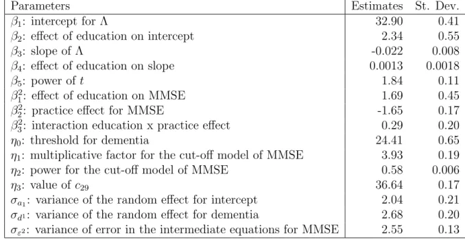
Table 2: Results from the analysis of the five-year follow-up of the PAQUID study

Parameters Estimates St. Dev.

β1: intercept for Λ 32.90 0.41

β2: effect of education on intercept 2.34 0.55

β3: slope of Λ -0.022 0.008

β4: effect of education on slope 0.0013 0.0018

β5: power of t 1.84 0.11

β2

1: effect of education on MMSE 1.69 0.45

β2

2: practice effect for MMSE -1.65 0.17

β2

3: interaction education x practice effect 0.29 0.20

η0: threshold for dementia 24.41 0.65

η1: multiplicative factor for the cut-off model of MMSE 3.93 0.19

η2: power for the cut-off model of MMSE 0.58 0.006

η3: value of c29 36.64 0.17

σa1: variance of the random effect for intercept 2.04 0.21

σd1: variance of the random effect for dementia 2.68 0.20

σε2: variance of error in the intermediate equations for MMSE 2.55 0.13

0 5 10 15 20 25 30 0 50 100 150 200 250 300 350 MMS

Figure 1: Histogram of the MMSE score at the initial visit. Black: observed histogram; grey: expected numbers.

65 70 75 80 85 22 24 26 28 30 32 34 36 38 40 42 MMSE=30 MMSE=29 MMSE=28 MMSE=27 MMSE=26 MMSE=25 MMSE=24 MMSE=23 age in year

Figure 2: Mean evolution of the latent process based on the follow-up of five years in the PAQUID study for low (dashed line) and high (plain line) educational level; the band (delimited by the dashed lines) shows a region where 95% of the values for low educated subjects lie; horizontal line with crosses is the threshold value for dementia; expected intermediate variables for subjects of low (stars) and high (open circles) educational level entering at 75 years in the study and seen at T0, T1, T3, T5 and T8; the grid shows the values of the MMSE obtained for specific values of the intermediate variable.

0 0.1 0.2 0.3 0.4 0.5 0.6 0.7 0.8 0.9 1 0 0.1 0.2 0.3 0.4 0.5 0.6 0.7 0.8 0.9 1 sensitivity 1−specificity

Figure 3: ROC curve showing the ability of the model to predict dementia at the eight-year visit based on the follow-up of five years in the PAQUID study