HAL Id: hal-02191403
https://hal-lara.archives-ouvertes.fr/hal-02191403
Submitted on 23 Jul 2019
HAL is a multi-disciplinary open access
archive for the deposit and dissemination of
sci-entific research documents, whether they are
pub-lished or not. The documents may come from
teaching and research institutions in France or
abroad, or from public or private research centers.
L’archive ouverte pluridisciplinaire HAL, est
destinée au dépôt et à la diffusion de documents
scientifiques de niveau recherche, publiés ou non,
émanant des établissements d’enseignement et de
recherche français ou étrangers, des laboratoires
publics ou privés.
To cite this version:
J.R. Burgan, J. Guttierez, A. Munier, E. Fijalkow, M.R. Feix. Group transformation for phase
space fluids. [Research Report] Note technique CRPE n° 47, Centre de recherches en physique de
l’environnement terrestre et planétaire (CRPE). 1977, 50 p. �hal-02191403�
CENTRE DE RECHERCHE EN PHYSIQUE DE
L'ENVIRONNEMENT TERRESTRE ET PLANETAIRE
NOTE TECHNIQUE CRPE/47
GROUP TRANSFORMATION FOR PHASE SPACE FLUIDS
par
J.R. BURGAN, J. GUTIERREZ, A. MUNIER, E. FIJALKOW, M.R. FEIX
C.R.P.E./P.C.E.
45045 - ORLEANS CEDEX
Le Chef du Département P.C.E.
C. BEGHIN
Le Directeur
GROUP TRANSFORMATION FOR PHASE SPACE FLUIDS
J.R. BURGAN, J. GUTIERREzf A. MUNIER, E. FIJALKOW, M.R. FEIX CRPE/CNRS - UNIVERSITE D'ORLEANS
INTRODUCTION
We want to study the time behaviour of Systems where long distances forces are prédominant. Such is the case of plasmas,
accelerator beam (where we are dealing with Coulomb forces plus elec- tromagnetic confinning external fields) and self gravitating gas (galaxy, cluster of stars etc...) where the Newtonian attraction compete against the thermal (ballistic)expansion. In many cases we can disregard the small irregularities due to the grain structure of the matter (with grain as big as a star in a galaxy) and describe the interaction through a continuous field obtained by the solution of the Poisson équation. This is the well known Vlasov Poisson structure where the global description is obtained by considering the distribu-
tion function f (x,v, t) in the 6 dimensional phase space in contra- diction to a regular
gas where we can usually deal with the first moments of f with respect to v (particles density, momentum, energy density etc...). Consequently we call phase space fluids such Systems. A discussion of the relative properties of thèse a priori very différent fluids is given in 111 and 121. From the model's maker point of view adopted hère they présent great similarities.
The non linear solution of the Vlasov Poisson Systems are of course very difficult to obtain analytically and most of the
studies resort to numerical simulation. As soon as we introduce nume- rical algorithme the problem is raised of the correction of the long time behaviour. From our expérience with differential équations this problem is best solved if we can find asymptotic séries based on a
systematic study of the différent terms. As a matter of fact we begin to mix both analytical and numerical method and find in this case possi- bility of following some Systems during thousands of period.
Our group is developping ideas along this line and preliminary en- couraging results are exposed in 131 141.
Another "cornerstone" upon which this paper is built is the existence of singular solutions of the équations. As indicated by their names singular solutions are to be opposed to the regular (usual) solutions. Singular solutions hâve a spécial ordinarily simple strucutre which is preserved during the motion. The problem is to know if thèse singular solutions are never représentative of the others (which at the beginning do not possess the spécial structure) or on the contrary are very représentative of the regular solutions which could for example go asymptotically to the singular solutions. There questions are of course pratically unanswered. In plasma physics the BGK structures 151 provides examples of such singular solutions. They are periodic steady state eventually moving at a constant velocity and self supporting.
Their stabilities is a very complex problem 111 and they can be "transient asymptotic" solution as shown by numerical experiments 161.
Steady state structures are usually not too difficult to obtain (although their number and their variety is a puzzle in plasma physics). Solutions involving the time are still more difficult.
Recently the group technique has been used both in plasma physics (but on fluid models of non linear waves rather that on Vlasov-Poisson
System) and on models which represent one dimensional équivalent of
Navier Stakes fluid Systems (Burger's, Kortweig De Vries équations etc...)
Although in there cases self similar group techniques solve the problem it is fair to mention that usually the problem had been already solved. Such is the case of the famous solitons structures 181 191. Incidently
the method must be traced back to Boltzmann who use it to solve the
heat diffusion équation.
Some confusion exists about the usefulness of the group method and the way the method should work. Usually we check tht symetry of the équations with respect to continuous transformation group. We subsequently, use this symmetry to reduced by one the number of variables. Numerical solutions are easier and sometimes analytical solutions are
- 3 -
one degree of freedom ve cannot say how thèse solutions are
affected by a modification of the initial (or boundaries) conditions.
We will consider the self similar transformations of the
phase space and more precisely we will consider the transformation
which will be justified later on. The meaning of the
transformation is such that the x,v?t dépendance can be condensed into a t,yT\ transformation where � and r) are the rescaled coordinates of the phase space and describe motion ao simple that the time behaviour can be consequently taken into account by this rescaling. In (1) T is an arbitrary time and it is convenient to consider that the initial time is not t = 0 but t = T. From the following considération it is clear that we are going simply to obtain généralisation of the BGK (steady state) structures.
In fact an interesting new point of view is to introduce both a rescaling like (1) and keep a time variation through the intro- duction of a new also rescaled time. In fact we will introduce the follo-
wing transformations
with a proper choice of 0(t), A(t), B(t) and C(t) \nder a slightly différent form. This transformation has an old story Introduced by
1101 it has been rediscovered by R.H. Lewis 1111. Our group has pointed out some of the interesting properties both from theoretical and
pratical point of view 131 1121. Now it appears under a new aspect and we will learn how to use the freedom
left (2) being really a continuous Lie group of
Now we end up this lengtly introduction with the title of the différent sections. In I we will review quickly some of the results of the classical self similar group theory applied to the Vlasov Poisson System (with the absorption of the time variation in the rescaling of the new phase space). In JT we will introduce the complète time phase space rescaling and will show the mathematical group structures. In III we will apply it to a very intriguing
problem of cosmological theory the structure of a self gravitating System when the gravitational constant G varies with time, and we will show that the Dirac hypothesis with G varying inversely with the âge of the universe corresponds to a very simple problem. In IV it will be shown that the problem of the motion of a charged particle in a unifarm in space, time varying magnetic f ield. is very similar to the precee- dings. In V we will généralise the group transformation introduced in III to the quantum case and in VI we will come back to the Vlasov Poisson System for plasmas (we will study non Linear oscillations for plane cylindrical and spherical geometry) self gravitating gas and the problem of the expansion of a beam under the space charge forces.
- 5 -
I - SELF SIMILAR GROUP
We consider a one dimensional collisionless phase space fluid described by the Vlasov Poisson System. This fluid may be an electronic plasma (where for simplicity we suppose a motionless ion background of density No) or a one species population beam. The two cases are respectively labelled P and B. The gravitational case labelled G is identical to the B case with a
chaînée of sign in the Poisson law. Consequently we hâve three independent variables x,v, and two fonctions f(x,v;t) the phase space distribution and E(x, t)
the electric field connected by the following Systems of équations
For simplicity we took e = m = £ = 1
As we mentionned already we introduce the transformation group
To get the formai invariance of the System we must consider the four following invariants.
in (4) a is a real arbitrary number. T is a characteristic time and it is useful to consider the time origin at t = T. At this time
From
(5) we see that the transformation is possible in the B case but not in the plasma case because the variable t is still présent in (5). Nevertheless a solution can be found in the following way we translate the time origin at T writing t = T+T. Assuming T -+ °° and keeping T finite (otherwise as large as we like) we see that 9.(t/T )2 - N0.AIoreover to avoid the trivial time indépendant solution
in (5) we must let ct - - with a/T =6, The transformation (4) becomes
and the Vlasov Poisson system becomes
Now équations (5) and
(7) should be discussed and f possible solved in the B and P case. This has been partly done in 1191 and 1201. An interesting solution is obtained taking a = -1 for the B case. Assuming that the self consistant field has the form
we get for the solution of F
This is the"phase space stick"structure discussed in 120 and generalised for a plasma in 1431. We see immediately that unphysical boundaries
conditions appear at � = ± - where particles whith infinité velocity are allowed to appear. It has been shown in \te\ that thèse difficulties can be partly overcame through the concept of contamination which is based on the fact that particles on the extremities do not contribute
to the field (as long as symetry is conserved). In fact this concept is going to be generalised and reiatroduced injjf and we will not discuss it any longer for the moment.
- 7 -
II - A USEFUL GROUP OF TRANSFORMATION
A) Dérivation of the transformation
Let us consider the transformations given by (2) where x and v are the coordinate and velocity of a particle. We hâve
We impose on'the transformation two conditions
1) The phase space élément should be conserved i.e.
implying that the Jacobian of the transformation must be unity ; this imposes
computing dv/dt and taking (9) into account.
2) We want to keep the Hamiltonian formalism.Consequently
Yld 19 = /7J and the new force ez àkf\/AQ must be a function of Ç and 9 only. Consequently, in the expression of aW/d9 the friction term i.e. the sum of the second and third terms in the left handside of
(10) must be zéro.
x and v being canonically conjugate we must again equal to zéro (B + -t-) v and consequently B = - dC/dt. From this last relation and (11) we deduce
which together with (9) defines completely the transformation cha-
racterised by the arbitrary function C(t). The "new field" Ë. acting on the particle in the new phase space, new time system is given by (12)
Sometimes we will need the divergence of e for Coulomb forces i.e. »
forces for which
From (14), x = � C and the relations
we obtain
in the B and G cases with d the dimensionality of the system (d = 1, 2, 3 respectively for one, two, three dimensional Systems) The case of an electronic plasma with a continuous ion neutralizing background of density No introduces a supplementary term
- 9 -
We will use extensively Eqs. (16) and (17). In the Vlasov description
�L �ft | -jF.J is replaced by 5..[(JJ"l.6) dl{ The fact that é\ Â*?- d7d"i/ shows that
f(ît, \J, t) - F Y? ', ^/�) and the Hamltonian équations = a 0 E= d^l/dO means that in the new phase space (with the new time) we keep invariant the Vlasov équation
B) Group structure of the transformation
Each élément of the transformation is characterised by the function C(t) which transforms
x,v, in Ç,r\,0. We can reiterate with another transformation characterised now by D(8) which
transforms � 11 6 in A y T. For a dimensional system introuucing
the unit matrix of rank d,i.e. I. We hâve for the product of the two transformations, for the new time,
For the new phase space the matrix transforming directly x_,v in Aj\i written.
The "new field" is given by
Taking into account
(22) can be written
From (19) (20) (21) and (23) we see that the successive applications characterised by C(t) and D(0) are équivalent to the application characterised by CD. This demonstrates the abelian group structure
of the transformation. Moreover being characterised by an arbitrary function C(t) the group is continuous.
C) Time and Forces renormalisation
In the new time, new phase space the motion équations are invariants and we can use ail the mathematical models developped up to now the only change will be in the computation of the force through Poisson law from (16) or (17). The new field is now the sum
of three fields.
The self consistent field of the System given through Poisson low is'computed in the same way except a multiplying factor C 4-d which varies with time.
� In the P case the background ion field is multiplied
by C .
- Moreover we must introduce a transformation field given
by
On the other hand the new time is given by
and we see that the time is rescaled. Since we want study the long time behaviour of the System we can choose C(t) such that 0 varies very slowly with t. In fact we can sélect C(t) in such a way that 6 goes to a limiting value
a renormalization of the time. This implies C(t) -+ °° with t and, of
course,this time renormalization is obtained at the expense of a force increase. We show that in some physical problems we can sélect C(t) to
renormalize) i.e. hâve a new time going to a finite limit, or at least si ow down considerably the time without introducing inf inities in the forces.
III - GRAVITATIONAL SYSTEM WITH TIME VARYING GRAVITATIONAL CONSTANT
We hâve seen that one conséquence of the transformation was to introduce a function C(t) which,elevated at a proper power,
scales the force. If a physical constant describing the interaction decreases with time C(t) can be selected as time increasing with
a balance between the two effects while 8 may go to a finite limit. In fact,for the Dirac hypothesis fthe problem of the dynamical évolution is very much simplified as if the Dirac law was an example invented to show the iâteres tof the group method. The Dirac hypothesis [141 1151 states that the gravitational constant varies with time accordingly
where t is the âge of the uni verse. We prefer to �hift the time and consider the présent time as origin. Then replacing t by t+ T with T = Q-I
From (16) considering a 3D system we can consider that in the new phase space the field is affected by the factor G(t) C(t). Taking G(t) C(t) = Go gives C(t) = 1 + fit and consequently the transforma- tion field vanishes But the new time 6 is now.
and goes to the finite limit 0, when t - 00. Consequently the study for ail time of a N body gravitating problem in the Dirac's hypothesis
is identical to the study of a N body gravitating System where G remains constant during a finite time interval equal to fi We
hâve been able to renormalize the time without introducing infinities in the force due to the time decreases of G. The Dirac law is the only one which allows to get rid of the variation of G without intro- ducing a transformation field. Ue hâve two possibilities : either we stick to the
x,v� space and introduce (25) or we consider the £ j.r|,0 space and consider G as strictly constant.
We will, of course, refrain from claiming that one space is more physical than the other. We must simply point out that 8 is
the éphémères time computed with the hypothesis of constant G. This time should be compared with the time given by an atomic clock,i.e. a time connected to the motion of électrons governed by electrostatic forces. The comparison of the two times was made by Van Flandern. Although it is very difficult get rid of the différent corrections,
this last author claims a residual différence between the two times supporting the Dirac's ideas with an fi = 101 years.
Coming back to the more technical problems of computing orbits when G varies with time,we consider the motion of mass point in 3 dimensions attracted by the origin with a gravitational constant given by
We sélect C(t) to be able to deduce the asymptotic properties and more precisely
-
To avoid increasingin time transformation field and G(e)
� Within this last constraint to compress the time as much
as possible with, if possible,a limiting
8,, Table 1 gives the
choice of C(t), the expression in the new variables 8^Ç,of the trans- formation field, of the gravitational constant
and^f inally, the relation
- 13 -
TABLE 1
For a..:?1the transformation field is
zerc� G(0) is constant or goes to zéro and 6 -
î - As a conséquence £ goes to a
limiting value ^ and the asymptotic trajectory is x = ^ (1+fit) with x increasing proportionally to the time.
In the case 1/2 �a �1 the gravitational constant decreases exponentially with 0 and the dominant field is fi 74 t. The asymptotic solution for � is consequently.
Combining with x = CÇ the selected value of C(t) in this case and coming back to the time t, we find that again x increases as fit. Consequently for a � 1/2 the asymptotic state corresponds to freely going particles with a uniform velocity. This is not surprising since G(t) - 0 when t -»- but this last condition is not sufficient. Indeed for a � 1/2 we will see that another type- of trajectory is possible. G(0) being a constant and the répulsive transformation field going to zéro for 0 - °°,we can predict two typer of trajectories. For the open one the gravitational field goes to zéro as Ç -2 while the transformation field goes to zéro as
Ç/02^ and in the case of � varying at least as 8 the transformation field, although going to
The asymptotic time évolution is given by solving
Seeking a solution of (29) of the form � = A8 we obtain Since for a �1/2^3 � 1 the domination of the transformation field is enhanced. Now introducing x = C� = ACe and expressing 6 as a function of t we obtain again an asymptotic solution in t for x.
But, of course, the initial conditions of the problem can be such that in the plane the trajectories are of closed type
The transformation field decreasing with 0 the asymptotic trajec- tory is an ellipse in � and altough G(t) - 0 the particle is still influenced by the center of attraction, turning around it with a distance going to infinity as (1+fit) .
IV - MOTION OF A CHARGED PARTICLE IN A UNIFORM IN SPACE, TIME VARYING MAGNE TIC FIELD
If a time varying G(t) is a simple hypothesis, the problem of a time varying magnetic field is certainly important from a practical point of view. Let as assume a uniform in space time varying magnetic field^B(t) = B(t) e.where e is a unit vector. Now a time varying B implies an electric field E = - 9A/3t. Since the vector potential is
we deduce
(30) must be handled with care. The electric field dépends obviously of the point of origin and is zéro on the line parallel to "e* and passing
through that origin. A priori B(t) being uniform it seems possible to take any point as the origin. The paradox is raised if we consider more carefullyhow the uniform magnetic field can be created.
- 15 -
Hère we consider a solenoid of length L and redius R where both L and R go to infinity. This configuration imposes a cylindrical symetry in the induced field and the axis of the Solenoid is
naturallv the line where E = 0. From
we obtain
Introducing (30) we see that
If we take C(t) in such a way that B(t) C 2 (t) = Bo (33) cancels and we obtain
and we hâve to treat the motion of a particle in a constant magnetic field Bo with the usual transformation field. Note that now C(t) is imposed by the relation
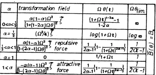
We investigate more precisely the case where
and we list on table II the value of the transformation field and the relation between 6 and t. [ln aH cônes the new magnetic field is Bo and C(t) = (l+fit)a ] .
TABLE II
In the new phase space for a � 1/2 the transformation field goes to zéro and the asymptotic trajectory is a circle (since B = Bo). Consequently, although the magnetic field goes to zéro, the particle will always feel its présence.
The case a = li/2 is quite interesting,(34) is written
Decoupling the motion in a first one perpendicular to the magnetic field (characterised by �l and �2) and another parallel (this last one is a trivial displacement at uniform velocity) we get the eigenfrequencies of the perpendicular motion w2
Solutions of (38) are .(¡ w = 1 E Bo+ Yst-Ji1 J . We must remember that due to the choice of units e = m = 1. Bo stands
for the cyclotron frequency (e/m) Bo. We find two possibilities.
- 17 -
1°) Bo � � ail theeigenvalùes are real and the particle undergoes oscillations in the £ plane. In the x plane x increase as aJL* Slt.
2°) Bo � fi two of the eigenvalues are complex and one corresponds to a growing instability in �. The particle has an asymptotic motion closer to the free motion. For B0 = 0 we recover of course the ballistic motion.
The asymptotic solutions for the case 1/2 �a � 1 is obtained noticing that the force is répulsive and that for 6 - 0 the motion is dominated by the transformation field
We seek a solution of the form
^ - A and obtain (3 = {cC-L)f(^oc - i) Taking into account the relation between 0 and t. this gives an
asymptotic solution for x = C� of the form x « fit indicating that the final-- motion of the particle is a ballistic free motion.
The last case a � 1 implies an attractive force. If we suppose that th� transformation field is still dominant (we will check a posteriori) we get the same équation (39) and the same value for 3 (but now is positive and the particle falls on the origin). The transformation field decreases like {9(-^)'J*�-^' _ (0f -8j "i« -4. while the magaetic force decreases as the velocity i.e.
(9* -6) "*�*-"�� "^ The ratio of the two forces (transformation/magnetic) varies as
lQf-9) and indeed for 6 - Of the transformation field is the dominant
one £ -� 0 as (0^- 9) �K*'(;'(i'3t"') and x = C� varies as fit împlymg in the regular x space a ballistic motion for large t.
Figures 1 to 5 illustrâtes this différent concept.
Figure 1, 2 and 3 shows what happens when a =.45. In ail cases -Q--4., For Bc = 10 the particles are nicely trapped in the plane indi- cating an expanding spiral motion in x. Notice that for Bo = 0.1
- 18 -
the particle gets on its circular orbit around 6 = 140. Such a value corresponds to t � 1012. This is an astonishing long time (and inci- dently supposes that the field stays uniform on the very large
corresponding distances).
4 4 and 5 illustrâtes the case a = .55. Hère the case B
= 10 is the interesting one. We see 14 révolutions in the t plane followed by the rather sudden escape of the particle". Again
the corresponding time is very large 6 = 8. t = 357 and practical space and time limitations will limit the possibility of seeing thèse transitions Nevertheless if is interesting to see that the Ç n 8 space with its high degree of compression in space and time is indeed the best suited for description of the motion.
V - THE GROUP OF TRANSFORMATION IN QUANTUM KECHANICS
A) Transformation of the Schroedinger équation
Let suppose one dimensional (to simplify) motion of a particle in a potential V(x). The description is through the Schroedinger équation
we introduce the
transformation ïrxC but dealing with the
Schroedinger formalism we cannot yet consider a relation between � and x and v (we will see later on).
Now we introduce the following transformation on ty
with
Computing -�i/0k ~ 3 //�// and introducing thèse results we obtain for the Schroedinger équation (40).
the "new Schroedinger équation" we want to write
consequently in (43) = (44) we must suppress the temr in
moreover equating the first terms in the right hand side of (43) and (44)
Finally getting rid of the terms in i�
Combining (46) (47) and (48) we obtain
while the potential V in (45) becomes
We see that as in the classical case the new potential is the sum of the rescaled physical potential V plus a transformation potential.
- 20 -
If we introduce the fields
i - � r - 9. r- -3 A
(52) is strictly identical to (14)
B) Introduction of the Wigner distribution function
How can we recuperate the second of équation (31) i.e. the relation between � and v and x ? The question is interesting and is answered by considering the Wigner distribution function 1161
-fCXiV).
It must be pointed out that the ^nysical meaning of this fonction is not clear since this function has not ail the good properties
characterizing such a distribution (the biggest difficulty being that f can be negative). From a Schroedinger � function Wigner defines a distribution in phase space through the relation
from (41)
We introduce (52) in (51) and use (50)
we introduce C -0 A and notice (49) that B C = 1 . We pbtain
Defining as in the classical case
and the phase space distribution is invariant as in the classical case. This is indeed the great advantage of the Wigner distribution:
The classical concepts can be used but of course the Wigner dis- tribution does not obey a classical Vlasov équation.
C) Application to the problem of quantum Harmonie oscillator with varying frequency
To end this section an quantum transformations let us consider a potential for a one dimentional oscillator given by
the classical problem involves the solution of the équation
Although the following resuit has already been established by Eewis and Riesenfeld 1171 let us show that if we know a solution
of (58) we can solve the quantum case. We transform the équation through a given C(t) and from (57) and (51) we get
If we choose C+jfL C. =� 0/ V - O ancj the problem is reduced to the problem of free particles. But a difficultyoccurs if C(Tj = 0
\ov fc -~Y 6 goes to infinity and we cannot pass t = T. Since another easy to solve problem is the quantum oscillator
with a fixed frequency 0. (t) = W2 we can sélect C as a solution of
and we hâve
y=iiOLç a problem with a known
solution. We must
simply solve (59). It can be shown that if C(0) � t) the solution of (59) never goes to zéro.
- 22 -
VI - VLASOV POISSON SYSTEM
A) One dimensional problem beam
We go back to the Vlasov Poisson system. We begin by considering a one dimensional beam problem B with an initial
condition as indicated on Fig. 6. It must be pointed out that we hâve put a limit V0 on the modules of the possible velocities.
Although physically such an absolute eut off does not exist the number
of particle with velocities greater than
saySVT is very small and can be supposed equal to zéro. Moreover the beam is limited in space from x=-Ltox=L and is homogeneous in this interval. To compute
its évolution we sélect a C(t)
such that C(0) = 1 and (dC/dt) -0 exfc (t = 0). At initial time
t = 0 =0 the two phase spaces x, v and Ç, r\ coincides. The
Poisson équation (17) can be
written FIG. 6 In thetplane at 6 = 0 F Lf , "\) - F("jJ /�** - L � | � £ |_ and the density] F d-it = N We sélect C such that*.
with C(0) =
1, dC/dt (0) = 0 . We get of course
If we remember that we took e = m = co = 1 we see that Q,2 is simply the plasma frequency associated to a density half of the initial density of the beam. Now the possibility of selecting such C(t) has two important conséquences.
The new field c is zéro and since the beam is uniform it will stays zéro. Being homogeneous and with no field acting on it the plasma is on a steady state with no time évolution.
In fact things are more complex. The steady state character of the beam implies a infinité length of the beam. If boundaries
exist,as they do; we must use the concept of contamina- tion already introduced in 181. We briefly remind it.
Due to the one dimensional character of the problem supposing moreover a space symmetry, particles outside a limited région do not create any field r.nside; this property remaining true in cylindrical. and spherical symmetrical structures. As long as thèse particles do not penetrate physically into this zone 'fhey will not influence the behaviour of the particles in this zone . VJhen particles located initially respectively in the inner and outer zones
cross a "contamination process" is generated. Obviously the évolution of the contaminated zones is given by the évolution of the two boun- daries and more precisely by the (symétrie) trajectcjfies of point A and B of Fig. 6. Now the trajectory of point A for example is a simple uniform motion (in the �, n, espace) with
and the régions |Ç| � ÇA is the uncontaminated zone. The interesting point is that:when t - 00 6 - limit et and the contamination will stop if L � V0 6, leaving the central zone 1 ç � L
-\Qg always
uncontaminated. Introducing (31) in (13) we obtain the relation
between 8 and t
and when t m- 1 A � ~^% . The percentage of uncontaminated particles in Fig. 6 is consequently 4 - "^ va mSLL
Fig. 7 and 8 shows an illustration of this concept. It can be noticed that in the usual phase space we hâve a simple expansion. Fig. 3 indicates that îndeed ai is an invariant. The computer experi- ments are of Lagrangian type with plane
superparticlesthe motion of
j*«3 7 -
[Evolution in the phase spaces xv (right) and xv (left) of an horizontal water bag rod. At t = 0 the cutt off velocities are ± Vo and the rad length is 2 L. We define Q as the plasma frequency corresponding to the density A Vo = 1/2 of the density at t = 0. (A being the value of the phase space density inside the bag). The problem is entirely characterized by the value of the parameter La/Vo (hère equal to 2). Figures are respectively given for Qt = a) 0 ; b) 0.5 ; c) 1.0; d) 1.5; e) 2.0. The uncontaminated zone is indicated only on the xv phase space and is a rectangle delineated by the straight lines ± Vo and the two vertical hnes whose abscisses are given by
± xJL = 1 - V,12 QL(t(1 + t2) + Arc tg r).
Hère for r -» ao the percentage of uncontaminated particles go to 1 - zV014 QL = 0.607 3.]
FiG.0
� Même diagramme xv que pour la figure 1 avec indication de l'évolution de 7 groupes de particules dont les vitesses initiales sont Vo, ± 2 V013, ± y a/3 et 0. On voit que dans la zone non contaminée û est un invariant.
B) One dimensional problem-plasma
For a plasma the corresponding Poisson équation (17) is written
Starting from a uniform électron plasma P as in Fig. 6
with an initial density n^ for the électrons and N for the mO�Û.t5nless ions we sélect C(t) satisfying C(0) = âJr(o) = 0 and
introducing the plasma frequency -O-p = N. e. /m Ê. the solution is
We see two things
If
ne/No � 1/2, C(t) will take the value 0 and for this value of the time, will be infinité. We will not be able to compute the behaviour beyond.
If
nD/No� � 1/2 C(t) is always positive but does not increase with timejwhen t - 00,8 + 00 and the contamination is alwavs total, irrespective of the System. The time of total contamination is L/V in the 8 scale. For the uncontaminated zone the density varies
°
-1 as n = n C (t)
The results are very similar to the cold plasma case 1181 with density in the centre oscillating at frequency �p. We notice that since C(U � �0im^(.�«» e-'7 o�J we always hâve total contamination before n(t) blows up in the case n /N o � 1/2.
- 25 -
C) One dimensional problem-gravitating gas
The case of gravitating gas with an initial situation described as in Fig.6 is similar to the B case except a sign
in front of N
= \Fdrn
and a solution for C(t) given by
fi is now the Jean's frequency associated to a" density equal to half the initial density of the System.
As in the B case the System is stationary in the �, n phase space with
n being an invariant in the uncontaminated zone. Of course the contamination becomes total in a time always smaller than Çl since the relation between 9 and t is now
If 2L is the length of the system the time of total contamination is given by the solution of the équation L/V
0 = 6. At time t the density in the incontaminated zone is N("f-..i2}.t2-;-1 and for a sufficiently large N a very large increase of the density
is consequently possible.Fig. 9 shows the situation for L SX./ U�� 4.. The invariance of n and the shrinking of the uncontaminated zone are well illustrated.
gravitational horizontal At initial time the boundaries are x = x = + L, v = v = + V . Hère the parameter characterizing the problem is ISi/V * 4. Figures, obtained using 3 000 a particle code are res- pectively given for Qx = a) 0. ; b) 0.3 c) 0.6 ; d) 0.9. In this case, the collapse and the crossing of ail particles in the neighbourhood of the center bring a total contamina- tion for JÎT = 0.92. It can be seen that, as long as the particles remain uncontaminated, v is an invariant. We indicate the évolution of seven groups of particles with initial velocities + V , + 2/3 V , + 1/3 V , and 0.
- 26 -
D) Homogeneous Systems in cylindrical and spherical geometry (Beam and gravitational gas)
An advantage of our group transformation analysis is that the results can be generalised to cylindrical and spherical geometry altough it must be pointed out that in order to apply the contamination concept we must deal with Systems where the particles from outside do not create a field for the particle inside who implies a cylindrical and a spherical geometry in respectively 2 dimensional and 3 dimen- sional problems. N being the initial density in the B and G cases with N/2 = fi and n. and N
o fi p the électrons and ion
density in theT case#Ve must select C(t) satisfying; in two dimensions (cylindrical)'.
O-t-
in three dimensions (spherical)
in ail cases C(t) and dC/dt for t = 0 are respectively ] and 0
DI) The two dimensional beam problem
In �he 2D B problem the relations between
C,' t and 6
C(t) 1 and C(t) an always increasing function with time goes to infinity when t - °°. � goes to a finite limit S\-�t = VTr and the contamination is only partial provided,of course, we can put a limit
V to the velocities and that R/V � � 0el The density in the uncontaminated zone is NC and this gives the law of decrease in the density under the influence of space charge and ballistic effect for a cylindrical beam.
D2) The two dimensional gravitating problem
In the two dimensional G problem, relations (73) and (74) are just inversed.
C(t) � 1 and C(t) an always decreasing function, with time equal zéro for -0Lt,=Vtr. Before that time/total contamination has taken places and up to that time we can follow the density increase in the center.
D3) The three dimensional beam problem
In the3dimensional B problem
Equation (72) B can be easily integrated giving
c(t) � 1 is always increasing. (9 goes to the finite limit v 6 SL and the contamination is partial. NC -3 gives the évolution of the density in the center of the spherical System.
D4) The three dimensional gravitational problem
In the 3D G problem, the intégration is quite similar to the preceeding one. We get
C(t) �� 1 is always decreasing. Contamination is total in a time always smaller than -CL't^ = IV \/J/F .
E) Plasma case : two and three dimensions
The plasma case is a little bit more difficult. We must solve(71)P,d being the dimension (d = 2 or 3)
Deriving (81) we get and cl1n/^t2-
Introducirig d^/^taken from (71) and (72) in (82)
we write P = dn/dt
Introducing (84) in (83) we obtain the first degree équation (P function, n variable)
The solution of which being
We must distinguish between d = 2 and d = 3
d = 3 gives no problem in the last intégration of (86) K is obtained noticing that for t = 0
n m- m. a~�L d n-/dt -~P= 0
We finally obtain the relation between t and n
The denominator of (88) cancels for n = n . It is easy to find the other values for which it is zéro. One is négative and without interest, the other is
(taking S\-=i,~i)
If rL. and if 11, �1 7), 4. A Consequently the density is periodic and oscillâtes between thèse two values. The period
is given by twice the intégral (88) taken between the values n o and n, 1 (or n, 1 and n0). In contradistinction to the plasma
case riç can be as small as we like without appearance of a maximum
n going to infinity (In the plane case n =
n /(2n -1). d = 2 is the last case to be treated. In (86)
(_,~a/�L iM
i *. Again we get
K throught t=0 //71-'7'La*el'I?=0.
- 30 -
t is obtained by intégration between n and n
As in the preceeding case the expression between bracketscancels for x =
n and x = n, (one greaterthe other smaller than N ) the density oscillâtes between thèse two values and is periodic with
the half period given by the intégral (91) taken from
n to n.
(or
n. to n ) . As in the 3 dimensional
cases no restrictions are put on the value of n ;and n infinity appear. (88) and (91) indicate that in cylindrical and spherical geometry the frequency of oscil- lation is a function of n in contradistinction to the resuit ob-
o
tained for plane geometry as given by (67)
where fi is
the oscilla-
tion frequency and does not dépend of n .
Nevertheless in the linearised limit we recover n
the 3 cases the plasma frequency � . The equation for C can be written
we suppose that Il. = II. (A t- E. ) =
XI.* (..4+ ê- ) and e is small
since n is very close to N . Introducing fi t = ~5 we rewrite (92)
we write C = 1 + � and linearize neglecting terms in i))2 1jJ3... (92) becomes
The solution of (94) with � = 0
Introducing (95) in n =
N ( J + £ ) C4 + t) -J.... and reta:LIli-I1g only the first terms in � we get
APPENDIX
SELF ADJUSTED TRANSFORMATION
1-. INTRODUCTION
We show in this appendix that the time rescaling of formulas (13) is a particular case of a more general theory of self adjusted transformation where we work directly in 4 dimensional space time
with the. coordinates and the time expressed as function of a parameter We indicate that it is possible to find a generalised canonical transformation for x y z*-««l "),.
2. CONFIGURATION SPACE C
Let
«=^o�y the generalized coordinates (1,4 =- t, h, "lit) they are indépendant variables in C space is then the set of ail the points M of coordinates q. Let us now hâve a relation ship between the q . This is the same as to give a parameter À, the variation of which des- cribes a curve in C. Thus each point M can be said to belong to a curve I of C, the position of M or Pis given by �, and the curve r itself dépends on the initial position of M.
A tangent vector along the curve H is
Thus : give a set of curves (i.e. a parametrization, i.e. trajectories), and get a tangent space.
The tangent base is ��.
Any tangent vector can read then x= 4 �=Tâ2
The dual tangent base is ci 9'
- 32 -
The exterior derivative of a scalar function f, along a vector field u is defined as :
2. PHASE SPACE W
According to Lagrangian formulation mechanics in Space- time trajectories dépend upon intégration of 4 second order partial differential equationl, thus dépend on 8 parameters.
Therefore we are bound to work in an 8 dimensional space (space and there coordinates, and momentum and Energy coordinates) Mechanical lows in 1E space are then given by
-
the knowledge of the Hamiltonian function H(p,q) - the application of a variational principe on the
1 form
this gives us the trajectories in phase space
which is nothing else than Hamilton's équations
3. GENERALIZED CANONICAL TRANSFORMATION
We know that Hamilton's équations are invariant under any canonical transformation which means that if we go over to new coordinates
°i�^lp) and
new rnomenta
K [ ^ , p) in such
a way as to hâve a canonical transformation, then
and we see that the parameter is still À.
We are now interested in transformationswhich are canonical in coordinates and moments but which also change the parameter to a new one; 7*
- 34 -
Therefore the transformation is defined by
relationship between � and "X (renormalized parametrization)
and by
generating function .
We restrict ourselves now to transformations
�9 t(çîi\) where the new coordinates do not dépend on the momenta. The trans-
formation is then
change of parameter
change of coordinate
generating function
If we write then
Then the new momenta are given by
and the new Hamiltonian is
The tangent space is generated by the Jacobian
note that in (q,p) space, directional derivative is defined by the )^ parameter, while in (q,p) space, it is defined by the parameter À.
Straight forward calculations give
If Hamilton's équations hold
in Q ( A)^p^) space, d % , H J � O
and
fp, HjrO» they hold too in cj(À)jp~(Â) space. But evi- dently the trajectories do not correspond in the two spaces.
4. APPLICATION TO PLASMA PHYSICS
We choose the following generating function
where p will be the momentum, canonical conjugate of the time variable t, this is the energy.
TrCare spatial momenta
;xLare the spatial coordinates
We hâve then
Therefore
we use now, along a trajectory, t as the parameter, thus A = t and we like to hâve, on the transformed curve X � ^-
Therefore, when we dérive
-f,- a (t}\)
- 36 -
we obtain
this is a ¡5torder partiel differential équation, which we can
integrate .
for A � t and for a judicious choice of constant "a we hâve :
if we now consider Vlasov's equation ;
Maxwell's equations:
with initial condition ;
and with normalization relation
Let us make the transformation :
as we hâve seen in paragraphe (3), Hamilton's équations in the new coordinates give a new Lorentz force
this results directly from the variation of the action S(x,t) which
The transformation law for the Halmitonian function
can be written :
We see that the energy is not conserved in the transformation and if H doestfiot dépend on t, H do dépend on 6. This peculiarity is due to the fact that we are dealing now with a new time parameter 9 which is not uniform.
We are able now to see that if the new electromagnetic field is defined as
Then Vlasov's équation is the same in the new variables.
The new electromagnetic field does not dépend on n, which was to be expected, since we like to hâve in the new variables a field depending only on the variables
(gr -
Clearly, two of Maxwell's équations are also immediately
satisfied :
The charge density becomes
and the current density becomes
The normalizing condition is also conserved, since the trans- formation is canonical and lets volume élément of phase space invariant.
- 38 -
CONCLUSION
We hâve seen in the body of the paper that the time rescaling was an interesting concept allowing to predictJana- tytically or numerically,certain asymptotic properties of a physical System. Usually we work in coordinate-momentum space and the time t is considered as the parameter, coordinates and momentum being expressed as function of t. Nevertheless, in
some situations (especially in problems involving general rela- tivity) it is simple to consider the time as a coordinate and to express everything as a function of a new parameter (proper time). We hâve shown that a rescaling of this parameter leaving invariant the canonical transformation formalism is also possible.
ACKNOWLEDGEMENTS
For fruitful discussions and coopération on the numerical simulation work the authors wish to thak Dr. M. NAVET.
We would like also to thank Miss F. FOURNIER for the ardous and meticulous typing of the manuscript.
1]1 M.R. FEIX, Some problems and methods in computational plasma physics. Proceedings of the Culham S.R.C. Sympo-
sium on turbulence and non linear effects in Plasma B.E. Keen and E.W. Laing Editors, pages 139-183.
J21 M.R. FEIX, Crossfertilization between Plasma, Stellar
Dynamics and Hydrodynamics,Dynamics of stellar Systems A. Hayli Ed.,Reidel 1975, pages 179-194.
131 J. BITOUN, A. NADEAU, J. GUYARD, M.R. FEIX, Jour. of Comp. Physics 12, 315-330, 1973.
141 A. NADEAU, J.P. VEYRIER, M.R. FEIX, Numerical and Analytical alternative to the Krylov Bogoliubov method. Applications to slightly non linear autonomous and monautonomous
Systems. 2nd European Conférence on Comp. Physics. D. Biskampf Ed. Munich April 76.
151 BERNSTEIN I.B., GREENE J.M. and KRUSHEL M.D., Phys. Rev. J08, 546 1957.
161 MORSE R.L. and NIELSON C.W., Phys of Fluids 12, 2418, 1969.
171 HSUAN H.C.S., LONNGREN K.E. and AMES W.F., Journal of Engineering Mathematics Vol 8, 303,1974.
181 SHEN H. and AMES W.F., Phys. Letters 49A, 313,1974.
191 ZABUSKY N.J. and KRUSKAL M.D., Physical Review Letters 15, 240,1965.
1111 LEWIS H.R., Jour. of Math. Phys., _9 1976, 1968.
1121 GUYARD J, NADEAU A., BAUMANN G., FEIX M.R., Jour.
Maths. Phys. 12, 488, 1971.
1131 BURGAN J.R., GUTIERREZ J., FIJALKOW E., NAVET M.,
FEIX M.R., Journal de Physique lettres
38, L 161
1977.
1141 DIRAC P. A. M. Proc. Roy. Society, A 333, 403, 1973.
1151 DIRAC P.A.M., Proc. Roy, Society, A 155 , 199, 1938.
|l6| J.E. MOYAL, Proceedings Cambride Philosophical Society, 45, 99, 1949.
1171 LEWIS H.R. and RIESENFELD W.B., Jour. Maths. Phys.
10, 1458, 1968.
1181 G. KALMAN, Anan. Phys 10, 1, 1960.
1191 V.B. BARANOV, Sov. Phys. Tech. Phys. 21, 720, 1976
1201 BURGAN J.R., GUTIERREZ J., FIJALKOW E., NAVET M.,
FEIX M.R., "Self Similar solutions for Vlasov and Water Bag Models". To be published.