Publisher’s version / Version de l'éditeur:
Vous avez des questions? Nous pouvons vous aider. Pour communiquer directement avec un auteur, consultez
la première page de la revue dans laquelle son article a été publié afin de trouver ses coordonnées. Si vous n’arrivez pas à les repérer, communiquez avec nous à PublicationsArchive-ArchivesPublications@nrc-cnrc.gc.ca.
Questions? Contact the NRC Publications Archive team at
PublicationsArchive-ArchivesPublications@nrc-cnrc.gc.ca. If you wish to email the authors directly, please see the first page of the publication for their contact information.
https://publications-cnrc.canada.ca/fra/droits
L’accès à ce site Web et l’utilisation de son contenu sont assujettis aux conditions présentées dans le site LISEZ CES CONDITIONS ATTENTIVEMENT AVANT D’UTILISER CE SITE WEB.
Gene Regulation and Systems Biology, 1, pp. 91-110, 2007-01-01
READ THESE TERMS AND CONDITIONS CAREFULLY BEFORE USING THIS WEBSITE. https://nrc-publications.canada.ca/eng/copyright
NRC Publications Archive Record / Notice des Archives des publications du CNRC :
https://nrc-publications.canada.ca/eng/view/object/?id=85f8f1a7-55dd-436f-a892-37e7d5237572 https://publications-cnrc.canada.ca/fra/voir/objet/?id=85f8f1a7-55dd-436f-a892-37e7d5237572
NRC Publications Archive
Archives des publications du CNRC
This publication could be one of several versions: author’s original, accepted manuscript or the publisher’s version. / La version de cette publication peut être l’une des suivantes : la version prépublication de l’auteur, la version acceptée du manuscrit ou la version de l’éditeur.
For the publisher’s version, please access the DOI link below./ Pour consulter la version de l’éditeur, utilisez le lien DOI ci-dessous.
https://doi.org/10.1177/117762500700100010
Access and use of this website and the material on it are subject to the Terms and Conditions set forth at Computational systems biology in cancer: modeling methods and applications
Correspondence: David S Wishart, 2-21 Athabasca Hall, University of Alberta, Edmonton, AB, Canada
T6G 2E8. Tel: 780-492-0383; Fax: 780-492-1071; Email: david.wishart@ualberta.ca
Computational Systems Biology in Cancer: Modeling
Methods and Applications
Wayne Materi2 and David S. Wishart1,2
1Departments of Biological Sciences and Computing Science, University of Alberta
2National Research Council, National Institute for Nanotechnology (NINT) Edmonton, Alberta,
Canada
Abstract: In recent years it has become clear that carcinogenesis is a complex process, both at the molecular and cellular
levels. Understanding the origins, growth and spread of cancer, therefore requires an integrated or system-wide approach. Computational systems biology is an emerging sub-discipline in systems biology that utilizes the wealth of data from genomic, proteomic and metabolomic studies to build computer simulations of intra and intercellular processes. Several useful descriptive and predictive models of the origin, growth and spread of cancers have been developed in an effort to better understand the disease and potential therapeutic approaches. In this review we describe and assess the practical and theoretical underpinnings of commonly-used modeling approaches, including ordinary and partial differential equations, petri nets, cellular automata, agent based models and hybrid systems. A number of computer-based formalisms have been implemented to improve the accessibility of the various approaches to researchers whose primary interest lies outside of model development. We discuss several of these and describe how they have led to novel insights into tumor genesis, growth, apoptosis, vascularization and therapy.
Keywords: cancer, computational systems biology, simulation, modeling, cellular automata
Background
Living organisms are complex systems. Nowhere is this complexity more evident than in the genesis and development of cancer. While cancer may originate from genetic and molecular changes that occur in a single cell, the subsequent proliferation, migration and interaction with other cells is crucial to its further development. In their landmark paper, Hanahan and Weinberg described six hallmarks they thought necessary for the transition from normal cells to invasive cancers (Hanahan and Weinberg, 2000). These included: 1) self-suffi ciency in growth signals, 2) insensitivity to growth inhibitory signals, 3) evading apoptosis, 4) limitless replicative potential, 5) sustained angiogenesis, and 6) tissue invasion and metastasis. While genetic instability was not explicitly included in this list, it was included as an implicit enabling alteration that might start a normal cell down a mutagenic pathway leading to the acquisition of one or more of these essential characteristics.
The molecules that govern the cell growth and division cycle in response to external and internal signals are numerous and interact through complex, multiply-connected pathways over a wide range of temporal and spatial scales. Tumors refl ect this complexity in that they are composed of several different cell types that interact to create malignant growth (Burkert et al. 2006). Despite the widespread acceptance of this complexity, the majority of biological and biomedical studies still utilize a strictly reductionist approach, focusing on the interactions of at most a few genes or proteins in each experi-ment. Systems biology, an integrative discipline that attempts to describe and understand biology as systems of interconnected components, has arisen partly as a response to these traditional reductionist approaches. Systems biology is a young fi eld made possible by the explosion of data from genomic, transcriptomic, proteomic and metabolomic techniques developed within the last decade (Hollywood et al. 2006; Bugrim et al. 2004; Jares, 2006).
Computational systems biology, which is a sub-discipline of systems biology, has developed both as a tool supporting the processing of these massive amounts of data and as a modeling discipline, building upon this “omic” data in order to predict biological behavior (Ideker et al. 2001a; Alberghina et al. 2004). Not surprisingly, both experimental and computational systems biology approaches have provided fruitful insights into cancer.
Please note that this article may not be used for commercial purposes. For further information please refer to the copyright statement at http://www.la-press.com/copyright.htm
This review provides an overview of how computational systems biology can be, and is being used to model cancer at multiple levels and scales, ranging from molecules to cells to tissues. Specifi -cally, we begin with a general description of the different computational modeling methods that can be used along with a discussion of their relative strengths and weaknesses. Following that, we describe some of the emerging formalisms, software and standards for representing biological systems. Finally, we provide a number of examples illus-trating how computational systems biology has enriched our understanding of a variety of cancer-related processes including genetic instability, tumor growth, apoptosis, angiogenesis and anti-cancer therapy. Overall it is our hope that this review will provide an improved understanding of modeling issues and thereby assist the reader in selecting an appropriate method for their own research.
Approaches to Computational
Systems Modeling
To be truly useful to a biologist or physician, computational modeling should: 1) produce useful predictions or extrapolations that match experi-mental results; 2) permit data to be generated that is beyond present-day experimental capabilities; 3) allow experiments to be performed in silico to save time or cost; 4) yield non-intuitive insights into how a system or process works; 5) identify missing components, processes or functions in a system; 6) allow complex processes to be better understood or visualized and 7) facilitate the consolidation of quantitative data about a given system or process.
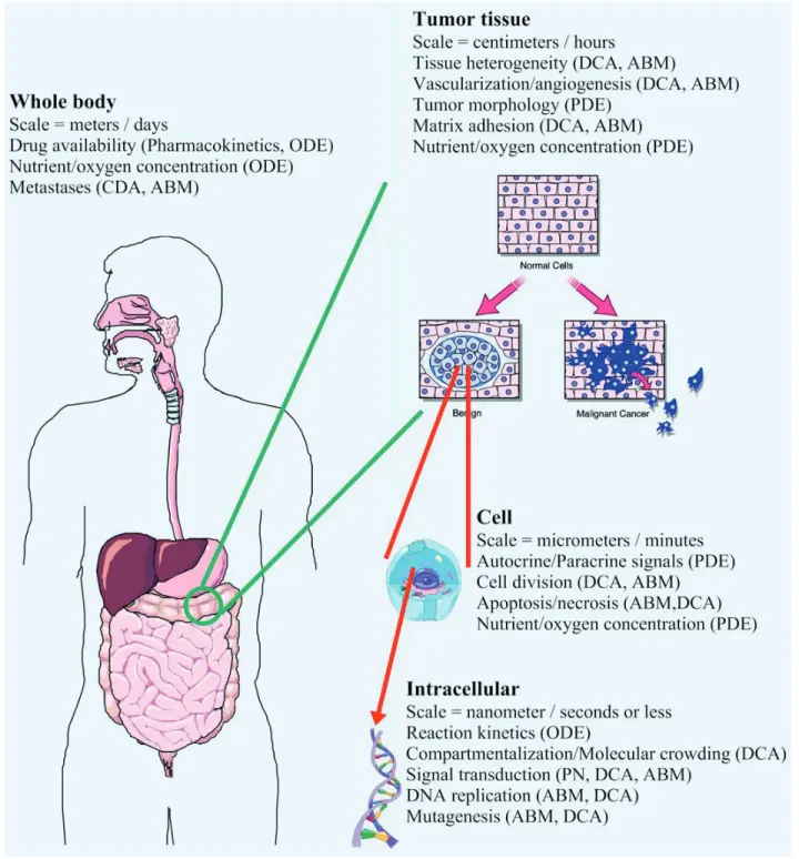
Simulations encompass many different spatial and temporal scales, ranging from nanometers to meters and nanoseconds to days (Fig. 1). Processes that occur over very small dimensions (nm) or short time periods (ms) are often referred to as “fi ne grain” models, while processes occuring over longer time periods (s) or larger (mm or cm) dimen-sions are called “coarse grain” models. A funda-mental challenge to computational systems biology is to develop models and modeling tools that can deal with this wide range of granularity. In this review we will describe some of the newer or more innovative modeling techniques that are being developed to permit both temporal and spatio-temporal modeling over this wide range of scales, including: 1) systems of ordinary differential
equations (ODEs), partial differential equations (PDEs) and related techniques, 2) Petri nets, 3) cellular automata (CA), dynamic cellular automata (DCA) and agent-based models (ABMs) and 4) hybrid approaches. Figure 1 presents an overview of scaling issues in modeling cancer and indicates which approaches are particularly well-suited to dealing with each area.
Building models of complex biological processes is an iterative process that requires considerable attention to detail. The network topology or struc-ture of a model may arise through literastruc-ture surveys or directly by computational analysis of high-throughput data (Wang et al. 2007—[Epub ahead of print]). In many instances such analyses may reveal novel regulatory or signal transduction interactions whose kinetics and stoichiometry is unknown (Janes et al. 2005; Kumar et al. 2007). Quantitatively accurate modeling requires explicit values for many variables including molecular concentrations, cellular distribution of molecules, reactions rates, diffusion rates, transport rates and degradation rates. While many of these can be estimated from the literature or various online databases, a number of parameters often remain unknown at the start of any simulation. As a result, many modeling processes require that one provide estimates for key parameters. Usually “best guess” fi rst order estimates can be used and then fi ne-tuned using a well-understood instance of the model as a comparison. Parameters are iteratively adjusted on subsequent simulations until the model accu-rately refl ects the known test case (Ideker et al. 2001a; Kunkel et al. 2004; Ideker et al. 2006). This period of validation is always required where any unknown parameters exist. However, a detailed discussion of network discovery and the model refi nement/validation process is beyond the scope of this review.
Computational modeling using
differential equations
Biological systems are essentially multicomponent chemical reactors and thus can be represented as systems of chemical reactions. This view permits mathematical analysis using powerful techniques developed from chemistry. Many standard biochem-istry texts provide thorough derivations of ordinary differential equations (ODEs) for both simple and complex reactions. In fact, ODE based modeling is the most common simulation approach in computational
systems biology, refl ecting both its rigor and adapt-ability (Kitano, 2002; De Jong, 2002).
Simple ODEs may have exact solutions. However, most complex ODEs do not have exact solutions and must be solved numerically. Based on methods fi rst derived by Newton and Gauss,
numerical integrators utilize linear approximations of smooth curves over small time intervals to compute subsequent values of reactant concentra-tions. Improving the accuracy of these linear esti-mates may require using smaller time intervals, leading to computationally intense processes that Figure 1. Issues of scale in modeling cancer. From whole organism to tumor tissue to individual cells to the molecules of replication and
metabolism, modeling tumors spans about nine orders of spatio-temporal magnitude. Shown above are some of the modeling issues which need to be addressed at each level of simulation. Each text box includes the relevant spatio-temporal scale and modeling issues encountered at that level. Appropriate modeling approaches to address each issue are shown in brackets. Building hierarchical systems of inter-related models is still a primary challenge to modern researchers. ODE – Ordinary differential equation system, PDE – Partial differential equation system, DCA – Dynamic cellular automaton, PN – Petri net system, ABM – Agent based model.
use considerable machine time. Various methods have been derived to improve the speed and compu-tational accuracy of these approximate methods, including Runge-Kutta algorithms and implicit methods (for so-called “stiff” differential equa-tions). These algorithms are encapsulated in such publicly-available packages as the LSODA (Liver-more Solver for ODEs with Automatic method switching for stiff and non-stiff problems) or CVODE (C Variable-coeffi cient ODE solver) inte-grators (http://www.llnl.gov/CASC/odepack/).
In addition to improved methods for solving general systems of ODEs, models of biological systems can take advantage of features specifi c to such systems. One such class of ODEs is called delay differential equations (DDEs). DDEs can reduce the computational effort required to model signal cascades, such as phosphorylation-dephosphorylation cycle networks (Srividhya et al. 2007). This allows the modeler to replace an intermediate signaling molecule (and all the ODEs associated with it) with a time delay term in the ODEs immediately preceding or following in the pathway. As long as the concentration of the inter-mediate is not a molecule whose concentration is tracked within the system, this results in no loss of information. By removing terms representing intermediate components in multi-stage processes, such as signal transduction cascades or mitosis, this approach reduces the number of equations to be solved and leads to more effi cient processing.
Systems of ODEs have been used to mathemat-ically model a wide variety of processes including metabolic pathways (Ideker et al. 2001b), mitosis in yeast (Tyson, 1991) and genetic regulatory circuits (Elowitz and Leibler, 2000). For example, as a representative MAP kinase signal transduction cascade, the ERK/MAPK pathway has been modeled independently by several researchers using ODE systems (Orton et al. 2005). Surprisingly, differences in construction details of various models, including number of molecular species and reactions, still led to similar results and predictions. It has been suggested that this is likely an indication of the general robustness of the ODE approach (Orton et al. 2005). Alternatively, this may refl ect the inherent robustness of biological systems themselves.
In many cases of biological or chemical modeling the kinetics can be described by a series of loga-rithmic or power law functions. As a result power law approximations of ODE systems have been
developed to improve the computational processing of this very common class of kinetic models. In this approach the rate of a reaction in the steady state can be estimated using Taylor series approximations of ODEs (Savageau, 1991). This leads to a system of non-linear equations where each rate is a product of non-integer powers of reactant concentrations and a coeffi cient. In a logarithmic coordinate system where the slope of the line represents the kinetic order of a particular reaction, the non-linear equa-tions can be readily transformed into a system of linear equations which can be numerically solved with little computer effort. These so-called S-systems have been used to model the TCA cycle in Dictyostelium discoideum (Shiraishi and Savageau, 1992; Shiraishi and Savageau, 1993) and to compute strategies for improving L-carnitine production in E. coli by altering media and biore-actor conditions (Sevilla et al. 2005).
S-system models can also be used to estimate coeffi cients and exponents associated with indi-vidual components when reaction rates are unknown. One such model used simulated annealing (SA), a process whereby initial estimates of coeffi cients and exponents are stochastically perturbed while the system is slowly “cooled” from an initial high pseudo-temperature (Gonzalez et al. 2006). SA methods permit the system to explore beyond local minima while the pseudo-temperature is high, then to converge towards local minima upon cooling. During the cooling period, model outcomes are compared to actual biochemical profi les using a least-squares error analysis. If the error for the current simulation is equal to or lower than that for the previous simulation, the current simulation is automatically accepted. If the new error is greater, it may still be accepted with a probability that is proportional to the pseudo-temperature.
Issues in ODE-based models
Both conventional systems of ODEs and their Power Law approximations do not automatically refl ect compartmentalization, transport and diffu-sion of molecular species unless explicitly speci-fi ed. This is because reaction kinetics equations, upon which these mathematical models are formu-lated, assume steady-states in well-mixed solutions with abundant reactants and few enzymes. The simplifi cations in standard representations of enzy-matic reactions (such as Michaelis-Menton equa-tions) incorporate assumptions about the relative
rates of intermediate steps which are independent of transient localized differences in concentrations. In reality, the cellular space even inside bacteria is crowded with macromolecules, having 300 to 400 g/l of macromolecules (e.g. protein and RNA) occupying 20 to 30 percent of cytoplasmic space, compared to the 1 to 10 g/l under which biochem-ists normally study reaction kinetics (Ellis, 2001). Macromolecular crowding strongly affects assump-tions about diffusion implicit in ODE-based modeling systems. For instance, one basic assump-tion in most models is that local concentraassump-tions of reactants or catalytic enzymes within the compart-ment are homogeneous. Even if local concentra-tions are explicitly modeled, diffusion rates for species of considerably different physical size are often assumed to be identical. Clearly, under crowded conditions, small molecule diffusion will be less impeded than that of larger proteins and protein complexes (Ellis, 2001).
Macromolecular crowding also affects reaction kinetics. Equilibrium rate constants for macromo-lecular association reactions under crowded conditions can increase by two to three orders of magnitude compared to dilute concentrations (Ellis, 2001). Thus the net effect of crowding on enzyme-catalyzed small-molecule reactions is a complicated function of the reduction in the rates of reactant diffusion and the promotion of enzyme-reactant transition complexes and is different for each reaction.
Within the cell, macromolecular crowding also leads to the formation of numerous non membrane-bound three-dimensional compartments and one-dimensional channels where reactions may occur. In addition, membranes can act as two-dimensional surfaces, leading to localized concentrations of proteins and complexes (Clegg, 1984; Srere et al. 1989). While conventional ODE systems and Power Law approximations do not inherently incorporate macromolecular crowding, they can be readily adjusted to a more accurate form using so-called “modifi ed fractal-like kinetics” (Schnell and Turner, 2004; Kopelman, 1988). This adjust-ment introduces a time-independent rate constant that refl ects the dimensionality of the reaction chamber (a measure of macromolecular over-crowding and compartmentalization).
Many biological molecules are present in very low concentrations (1 – 10 nM within the cytoplasm, which translates to fewer than 100 molecules per cell). Classical ODE solvers are highly unstable
and may fail to accurately refl ect the granularity and discrete system behaviour typically found at such low concentrations. Because of this, some modelers have added “noise terms” to their systems of equations by using so-called stochastic differ-ential equations (SDEs) (Meinhardt and De Boer, 2001; Chen et al. 2005). An alternative and widely-used approach to introducing stochasticity into a system of ODEs is to introduce a “master equation” derived from a “grand probability function” (Gillespie, 1976). The Stochastic Simulation Algo-rithm (SSA) is a simple method for selecting which reactions will occur in a given time interval based on such a master equation. For each reaction, the SSA method calculates P(t,µ), the reaction prob-ability density function; where P(t,µ)dt = the probability that, given the state (X1, X2, … Xn) at time t, the next reaction, will occur in the infi ni-tesimal time interval (t + τ, t + τ + dτ). For any reactant in any time interval in a chemical reaction system P(τ,µ) can be calculated in a straightfor-ward fashion from a uniform pseudorandom generator (see Gillespie (1976) for a complete derivation).
SSA methods have been used to model a variety of processes, including PKC signal trans-duction (Manninen et al. 2006), MAPK signal transduction (Chatterjee et al. 2005), and Hox gene expression in the developing vertebrate hindbrain (Kastner et al. 2002). Although SSA methods are accurate, they are computationally intensive. Chatterjee et al. have developed an explicit bino-mial tau-leap method to accelerate SSA models by two to three orders of magnitude and demonstrated this improvement in a MAPK cascade simulation (Chatterjee et al. 2005). This algorithm computes transition probabilities per unit time for a reaction system, then allows a “bundle” of events sampled from a binomial distribution to occur simultane-ously in the next time interval τ. This bypasses the dominating effects of fast kinetics reactions in the SSA model and emphasizes slower reactions that are likely of more interest to the modeler. Gillespie has recently reviewed several improvements to the original SSA method as well as implicit tau-leap methods (Gillespie, 2007). He has also introduced slow-scale SSA methods, an approximation that is applicable only for stiff ODE systems but which also result in accelerations of two to three orders of magnitude in solution time.
A key limitation of ODE-based models is that they only allow for one independent variable in a
system. As a result, most ODEs represent changes in the concentration of some chemical species varying over the independent variable time. Systems of partial differential equations (PDEs) must be used if one wishes to incorporate explicit spatial distribu-tion of components into a model. PDEs have been used to model several processes in cancers, including chemotactically-directed tumor growth (Castro et al. 2005), growth factor-stimulated glio-blastoma growth (Khain and Sander, 2006), the tumor-immune system interaction (Matzavinos et al. 2004), and tumor growth along tubular structures (Marciniak-Czochra and Kimmel, 2007). Due to the increased complexity and number of variables, PDE solvers are even more computationally intensive than ODE solvers.
Historically, the effort and mathematical skill required to set up a useful ODE or PDE model put this approach beyond the reach of most experi-mental biologists. However, recent advances in graphical interface (GUI) design, improved stan-dards in displaying and generating reaction models along with the development of standardized mark-up languages such as SBML (Systems Biology Mark-up Language) and Cell-ML (Cell Mark-up Language) are making the generation and exchange of interesting biological models relatively simple (Schilstra et al. 2006). A large repository of ODE-based Cell-ML metabolic and cell signaling models has been compiled at the Cell-ML model repository website (http://www.cellml.org/examples/reposi-tory/) as well as in the JWS online system (http:// jjj.biochem.sun.ac.za) which is part of the silicon cell project (http://www.siliconcell.net) (Snoep et al. 2006). Additionally a large number of SBML models are located at the BioModels website (http://www.ebi.ac.uk/biomodels/). Table 1 provides a list of common ODE simulation pack-ages, many of which are compatible with SBML or Cell-ML.
Computational modeling using
petri nets
Petri nets are a discrete alternative for representing time-dependent processes such as those occuring within biological systems (Moore et al. 2005). Petri nets, which were originally developed in the 1960’s, have long been used to model discrete distributed flow systems such as data-communications networks and manufacturing processes. It wasn’t until 1993 that biologists realized that this modeling
approach could be easily adapted to representing biological systems (Reddy et al. 1993). A Petri net contains two kinds of nodes, called “places” and “transitions”, represented graphically by circles and rectangles, respectively. In a molecular model each place is a species of molecule with some number of tokens inside, representing the number of mole-cules or concentration of that species (called the “marking” of that place). Transitions represent reactions. Places are connected to transitions by arrows (or “directed arcs”) either from source (input) places into the transition or from the transi-tion to product (output) places. The stoichiometry of a reaction is indicated by a weight on the arc. Because it is a discrete system, it is driven in step-wise fashion by implicit time increments. A transi-tion “fi res” (i.e. the reactransi-tion occurs) when the markings at all its input places are greater than the weights on its input arcs (ie when there are enough source molecules), producing product of the appro-priate weights on its output arcs (which are subse-quently stored in the product places).
Petri nets were originally designed to model discrete processes but later enhancements have added the ability to deal with continuous quan-tities (Goss and Peccoud, 1998; Matsuno et al. 2003). In addition, the basic Petri net formalism has been extended to deal with many of the complex issues that also arise in ODE-based models (Pinney et al. 2003). Hybrid Petri Net and Functional Hybrid Petri Net (FHPN) models allow markings in places to take either discrete or continuous values, thus permitting equivalent modeling power to ODE-based systems (Doi et al. 2004; Matsuno et al. 2003). Timed Petri Nets allow the implicit incorporation of deter-ministic delays in firing transitions, similar to those incorporated in DDE systems. Stochastic Petri Nets control transition firing with an expo-nentially-distributed time delay, equivalent to “chemical master equation” approximations of stochastic behavior in ODEs (Goss and Peccoud, 1998; Kurtz, 1972). Colored Petri Nets, which are an extension of Hybrid Petri Nets, allow for the definition of mathematical relationships inside transitions governing the rate of firing (Lee et al. 2006). Finally, Hierarchical Petri Nets are intended to support the composition of more complex models using combinations of previous models. No single implementation provides support for all variations. Further, compartments can only be represented explicitly, where
different places represent the same chemical species in different compartments.
Petri Nets have been used to model a wide range of biological processes, including qualitative modeling of apoptosis (Heiner et al. 2004), iron homeostasis (Sackmann et al. 2006) and the yeast mating response (Sackmann et al. 2006). FHPNs have been used to model several biochemical processes, including the E. coli lac operon (Doi et al. 2004), urea cycle disorders (Chen and Hofestadt, 2006) and p53 transcriptional activity (Doi et al. 2006). Koh et al. have used FHPNs to model the AKT and MAPK pathways (Koh et al. 2006). Using an evolutionary parameter selection technique and pathway decomposition these authors were able to determine optimal parameters for the model. Subsequent simulations suggested that Akt-MAPK crosstalk is required for enabling the Akt-MAPK pathway. Colored Petri Nets have recently been used for quantitative modeling of the EGF signal transduction pathway in an effi cient and dynamic manner using rate equations inside transitions that are highly reminiscent of ODE-based SBML or CellML systems (Lee et al. 2006).
Computational modeling using cellular
automata and agent based models
An alternative approach to modeling the complex systems of discrete molecules that are
found in living organisms is to use cellular automata (CA) to represent individual molecules and the rules that govern their interactions. Cellular automata (CA) are simple computer simulation tools that can be used to model both temporal and spatio-temporal processes using discrete time and/or spatial steps. Cellular automata were invented in the late 1940’s by von Neumann and Ulam (Rucker and Walker, 1997) who conceived of an infinite lattice of points (or cells), each capable of a finite number of states. Each cell is connected to a finite number of neighbors whose collective states at time tn induce it to assume a new state at time tn+1 in a specified manner. In biological systems the lattice represents two- or three-dimensional volumes in space and each cell can contain one molecule or biological cell (or sometimes more). So-called “lattice-free” systems use the lattice to represent real, physical space and individual entities may span more than one cell (i.e. more than a single x,y,z coordinate). Time is a discrete entity in CA models. At time tn the state and neighbors of each cell are tallied and rules applied to determine the state transition for that cell in the next interval tn+1.
Rules of varying complexity govern the interac-tions between adjacent or nearby molecules. Rules may be quite simple, for example, specifying binding of adjacent molecules with a certain probability
Table 1. Partial list of computational systems biology simulation software packages.
Method Package URL and reference
ODE, PDE, SSF Cell Designer http://www.celldesigner.org/index.html (Kitano et al. 2005) CellWare www.cellware.org (Dhar et al. 2004)
Dynetica http://www.duke.edu/~you/Dynetica_page.htm (You et al. 2003) E-Cell http://www.e-cell.org/ (Tomita et al. 1999)
Gepasi http://www.gepasi.org/(Mendes, 1993)
SmartCell http://smartcell.embl.de/ (Ander et al. 2004) VCell http://www.vcell.org (Loew and Schaff, 2001)
MesoRD http://mesord.sourceforge.net/index.phtml (Hattne et al. 2005)
Dizzy http://magnet.systemsbiology.net/software/Dizzy/ (Ramsey et al. 2005) Petri Net, Snoopy http://www-dssz.informatik.tu-cottbus.de/index.html?/software/snoopy.html
CPN Tools http://wiki.daimi.au.dk/cpntools/cpntools.wiki (Lee et al. 2006)
Cell
Illustrator-Animator http://www.gene-networks.com(Peleg et al. 2005)
DCA and ABM CancerSim http://www.cs.unm.edu/~forrest/software/cancersim/ (Abbott et al. 2006) MCell http://www.mcell.cnl.salk.edu/ (Stiles and Bartol, 2001)
SimCell http://wishart.biology.ualberta.ca/SimCell/ (Wishart et al. 2005)
AgentCell http://fl ash.uchicago.edu/~emonet/biology/agentcell/ (Emonet et al. 2005) Hybrid Cell++ http://www.compsysbio.org/CellSim/ (Sanford et al. 2006)
(Wishart et al. 2005). Alternatively, more complex rules can be formulated. For example, interactions of molecules may take place in a distance-dependent manner, representing biophysical relationships more accurately (Broderick et al. 2005).
In order to realistically simulate complex systems of reacting molecules, stochasticity needs to be added to the deterministic rules of the original cellular automata formalism. Dynamic Cellular Automata (DCA) permit “Brownian-like” motion of individual molecules through the incorporation of a random number generator which selects a direction of motion in the next time step (Wishart et al. 2005). Depending on the implementation of the DCA algorithm, molecules may move one or more cells in a single time step.
Chemical reaction rates are emergent proper-ties of DCA models although molecular reaction probabilities may be derived from conventional reaction rates. However, given the problems in deriving biologically relevant reaction rates that take into account macromolecular crowding, extremely low concentrations and compartmen-talization, it may be more accurate to compute parameters that match the biochemical profi le of a well-known test model.
DCA models have been used to model a wide variety of processes including diffusion (Kier et al. 1997; Wishart et al. 2005), micelle formation (Kier et al. 1996b), basic enzyme kinetics (Kier et al. 1996a; Wishart et al. 2005), myxobacteria aggrega-tion (Sozinova et al. 2005), osmotic shock (Broderick et al. 2005) and HIV/AIDS progression and treatment in single patients (Sloot et al. 2005). Both metabolic processes and simple genetic circuits have been modeled using estimates for reaction probabilities based on general kinetics or empirical values (Wishart et al. 2005). The results in all these cases have proven to be surprisingly accurate despite the apparent simplicity of the models, proving the power of the DCA approach.
Models of complete cells, even simple bacteria, could potentially incorporate billions of indi-vidual molecules. Interactions between molecules must be specifi ed in a computationally effi cient manner if such models are to compete with solu-tion times for the mere hundreds of equasolu-tions potentially found in comparable ODE systems. Nonetheless interactions must be fi rmly based on real forces or accepted approximations. For example, a recent DCA model of lipid bilayer dynamics in a 60 nm diameter proto-cell with
over 10,000 individual components used the Lennard-Jones potential as the basis for attractive and repulsive forces to realistically model the membrane (Broderick et al. 2005).
Agent Based Modeling (ABM) is similar in concept and design to Dynamic Cellular Automata. In ABMs genes, proteins, metabolites or cells can all be “agents”. Agents are allowed to interact with each other over space and time according to a pre-defi ned set of rules. The motions may be directed or random (Brownian) and the rules may be simple or highly complex. Unlike CA models, agent based systems do not formally require spatial grids or synchronized time steps, although practical coding considerations usually force these constraints on ABMs. Space is usually represented in a lattice-free grid. ABMs share many of the same advantages and disadvantages as DCA or CA models. Agent-based models have been used to simulate bacterial chemotaxis (Emonet et al. 2005), to model the calcium dependent cell migration events in wound healing (Walker et al. 2004) and to predict clinical trial outcomes of different anti-cytokine treatments for sepsis (An, 2004).
Hybrid Approaches
ODE, Petri Net, DCA and ABM approaches all have their unique advantages and disadvantages. While DCA and ABM systems have molecular-grain accuracy and implicit simulation of compart-mentalization, diffusion and stochasticity, they can also be computationally more intensive as the number of components in a model can increase rapidly (Ridgway et al. 2006). ODE systems ideally represent dilute reactants in single compartments, though effi cient methods have been developed for approximating more biologically realistic models. Nevertheless, ODE systems do not generally capture the true granularity or stochasticity of living systems and do not usually provide adequate visual feedback so important to developing clear conceptualization (Wishart et al. 2005).
A number of researchers have recommended hybrid or hierarchical hybrid systems to combine the strengths of both discrete and continuous approaches (Coveney and Fowler, 2005; Ridgway et al. 2006; Sorger, 2005). For example a simula-tion of bacterial biofi lm development was devel-oped where soluble substrates were represented by PDE systems in four spatio-temporal dimensions while bacterial cell growth was modeled seperately
defi nition (specifi cation available at http://source-forge.net/project/showfi les.php?group_id=71971) which incorporate Content MathML (http://www. w3.org/TR/MathML2/) and Resource Description Framework (RDF – http://www.w3.org/RDF/) for metadata description, only made this situation worse. Fortunately a large number of support programs have enabled biologists to define components of an SBML system using simple graphical descriptions of reactions and compart-ments that are much more easily interpretable. Links to web-sites supporting SBML models can be found at http://www.sbml.org.
For simulation purposes SBML is strictly ODE-based. Despite this restriction, a large variety of SBML-related modeling programs have arisen for the purpose of actually running simulations defi ned in the formalism. SBML handles compartmental-ization of reactants through its use of a KineticLaw reaction defi nition which incorporates compart-ment volumes into standard reaction rate equations (Finney et al. 2006). However, while rate equations for simple compartmentalized reactions may be converted easily to a corresponding KineticLaw, more complex reactions may require specific knowledge of compartment transfer rates. Both continuous and discrete models can be defi ned in SBML though they require different representa-tions of the corresponding rate equarepresenta-tions. A repository of published and unpublished SBML models is maintained at http://www.ebi.ac.uk/ biomodels/ which can also be reached from the Biomodels web site http://www.biomodels.net/ (Le Novere et al. 2006).
CellML is a an example of another XML-based formalism developed through the International Union of Physiological Sciences (IUPS) Human Physiome Project (Hunter et al. 2002; Lloyd et al. 2004). CellML models networks of interconnected components whose behavior is described by math-ematical equations written in Content MathML 2.0, a subset of which is embedded within the CellML framework. These features make CellML particu-larly amenable to modeling electrophysiological systems though it readily incorporates chemical reactions and gene networks. In addition, CellML provides for the inclusion of metadata (i.e. data describing the model, itself) within the model. This may include data derived from publications and ontological or semantic descriptions, such as keywords. Many of these features have now been incorporated into SBML Level 2 as well. with a deterministic CA (Picioreanu et al. 1998).
This model accurately refl ected global oxygen consumption as well as the concentration profi les of substrate and biomass. The distribution of the bacterial cells in relation to substrates and inocula-tion density were also accurately predicted. A primary benefit from hybrid models is the ability to integrate processes that occur rapidly (e.g. diffusion) with processes that can take days (e.g. cell growth and migration). This mixing of scales of time and space is normally one of the most significant impediments to accurately modeling biological processes using reasonable computer power (Coveney and Fowler, 2005).
Biological systems can also be viewed as complex control systems whose rules can be repre-sented using so-called “fuzzy logic” (Sproule et al. 2002). Fuzzy logic permits the use of qualita-tive terms such as “high” or “low” concentration to be incorporated into models. A hybrid model incorporating inference rules and fuzzy logic has recently demonstrated the utility of this approach by modeling sonic hedgehog signaling in the development of medulloblastomas (Bosl, 2007).
Formalisms for Representing
Biological Systems
Most biologists are not comfortable representing molecular systems using many of the mathemat-ical tools described above. Further, most models have been developed without consideration for integration with models developed by other groups. To address these issues, Hucka, Finney and others formed a Software Platforms for Systems Biology forum in 2000 where they fi rst proposed the development of SBML or Systems Biology Markup Language (Hucka et al. 2003; Finney and Hucka, 2003). SBML is a simple formalism (language) for describing networks of chemical reactions occurring inside biological entities. It uses the widely-accepted XML (eXten-sible Markup Language) representation to defi ne compartments, molecular species, reactions, parameters and rules (Webb and White, 2005).
Representing a simple reaction such as
A B+ →k1 C is not a trivial process in SBML.
Even ignoring supporting statements, describing this single chemical equation still requires a rela-tively large amount of SBML code. In addition to being long, the code is largely unreadable to the novice. Level 2 enhancements to the SBML
An important part of the CellML philosophy (besides providing a clear, consistent, verifi able formalism) is to encourage hierarchical composi-tion of models. This allows one to combine previously developed models in workable combi-nations (Lloyd et al. 2004). CellML’s encapsulation grouping structure is somewhat reminiscent of modern object-oriented programming languages. Version 1.1 of CellML also introduced the import feature to allow for components and connections to be reused in new models.
The modeling power of CellML is based on the ability to explicitly defi ne the mathematical rela-tions between all components. Compartments within a cell are considered components into which other components may be grouped. Thus, move-ment of components between compartmove-ments must be defi ned explicitly. Stochastic modeling is not yet supported by CellML nor is the modeling of discrete objects. The CellML and SBML project teams are cooperating to incorporate each other’s strengths, where possible, and to provide for models in one formalism to be translated into the other (Schilstra et al. 2006). Complete specifi cation of the CellML language can be found at http:// www.cellml.org/specifications and over 350 models are currently contained in a repository at http://www.cellml.org/models/.
No single formalism represents the Cellular Automata approach to modeling Usually the defi ni-tion of each CA formalism is encapsulated in its specifi c implementation. Recently, however, some effort has been made to formalize a more consistent approach to generating and sharing hybrid CA models of cellular processes (Cho et al. 2005). This hybrid approach allows both discrete and continuous components, constraints, stochasticity, regulation of transcription and mutations in a mathematical framework. However this system has only been used to model a small reaction system and it is uncertain whether it could be readily extended to more complex processes. Overall the CA fi eld continues to be dominated by insular approaches to specific problems. This should not be too surprising given the fact that the cellular automata approach is more concerned with an implementation philosophy rather than notational representation. On the other hand proponents of CA emphasize that continuous values are actually emergent properties of discrete processes and that a CA approach would result in truer models (Wolfram, 2002). Others have suggested that multiple formalisms incorporating,
for example, ODEs for physiological and chemical changes but CA formalisms for discrete cells in a tissue may lead to the best compromise between biologic accuracy and implementation speed (Defontaine et al. 2004).
Frequently, translation into a specifi c formalism is the most diffi cult step in converting a drawing of some process into a formal model for that process. The notation systems for all formalisms look nothing like the diagrams that biologists and biochemists are used to (with the exception that biochemists may be somewhat familiar with ODE representations of chemical reactions). Fortunately computer-based graphical tools have been devel-oped permitting the entry of a model with symbols familiar to biologists (or easily learned) and subse-quent machine conversion into a particular formalism. A number of these are listed in Table 1 along with web sites from which they can be down-loaded or run.
In addition to defi ning a model, simulation requires some computer program to run the model over a period of time or iterations producing output for interpretation. Output usually consists of graphs of the concentration of some component over time (or number of molecules, for discrete models) but may also include dynamic representations of the system or other analysis. The programs listed in Table 1 all include or can be linked to a variety of simulation modules. Reviews comparing specifi c features of some of these systems have been published (Peleg et al. 2005; Alves et al. 2006). In addition, a number of specifi c SBML tools have been developed, including SBML ODE Solver (Machne et al. 2006), MathSBML (Shapiro et al. 2004), SBML ToolBox (Keating et al. 2006), SBW-MATLAB interface (Wellock et al. 2005), SBML-PET (parameter estimation tool) (Zi and Klipp, 2006), and various other tools for programmers wishing to connect to SBML or the Systems Biology Workshop (SBW) (Gillespie et al. 2006). The availability of these tools (http://sbml.org/ index.psp) should make computational systems biology far more accessible to a much larger community of life sciences researchers.
How has Modeling Informed us
About Cancer?
As was noted earlier biological simulations should not be considered as simple academic exercises. Rather they should aim to inform researchers about
some unobvious characteristic of the simulated process. It is appropriate to ask, then, how models of cancer have led to novel insights into the disease. In the following section we review how modeling and computational systems biology has contributed to our understanding of the underlying molecular, cellular and tissue-level mechanisms of cancer.
Genetic Instability
The contribution of genetic instability to the devel-opment of cancer is controversial. Estimates of the number of mutations acquired in cancer cells range from 104 at the lower limit to a maximum of about 1012 (Abbott et al. 2006). A simple ODE model has been developed to explore the kinetics of tumor progression and to compare the importance of genetic instability compared to other factors such as avoidance of apoptosis, increased growth rate or angiogenic signaling (Spencer et al. 2004). The 17 equations in this model incorporated a muta-genesis rate which resulted in various advanta-geous mutations. Following acquisition of the genetic instability mutation, the global rate of mutagenesis was increased. Surprisingly, the model demonstrated that genetic instability was only important in the development of late-stage sporadic tumors, as it confered no general survival advan-tage to altered cells in the early sadvan-tages of cancer.
A separate study led to a similar conclusion on the basis of examination of the karyotype of populations of cancer cells (Heng et al. 2006). Rather than instability associated with individual genes, large-scale chromosomal instability was shown to make a more important contribution to early development of pre-cancerous cells. Clonal expansion and avoidance of apoptosis was criti-cally required for early tumor development as these characteristic allowed unstable cells to exhibit any acquired survival advantages. These ODE models did not, however, incorporate removing replication limits on cancerous cells nor metastasis, but proposed that agent-based approaches might model these characteristics better.
A direct test of increased genetic instability in tumor tissues has recently been conducted in trans-genic mice that produce mammary tumors with high frequency (Stringer et al. 2005). These mice were also transgenic for a mutant allele of human placental alkaline phosphatase incorporating an insertion of an 11 base pair G:C tract. This insertion caused a frameshift which rendered the protein
inactive. Loss or insertion of base pairs due to an increased mutation rate (resulting from genetic instability associated with cancerous cells) could restore gene function and allow such cells to be visualized in situ in tissue sections. A simple probablistic computer model predicted that many islands of individual staining cells, rather than only a few large clusters of staining cells, should predominate in tumors if genetic instability were more important in early-stage cancers than increased proliferation or apoptotic avoidance (Stringer et al. 2005). In the aggregate, across 17 tumors examined, the frequency of cell clusters of the predicted size matched the predictions of this simple genetic model. However, individual tumors exhibited extreme variability in cluster population, suggesting that hyperproliferation and survival were more important than genetic instability in many tumors.
A more recent stochastic cellular automata model based on Hanahan and Weinberg’s “hall-marks of cancer” was proposed to resolve the issue of the importance of genetic instability (Spencer et al. 2006). A 100 × 100 × 100 grid representing a maximum of 106 cells was initialized with a single cell, a single blood supply for nutrients and a limited growth factor supply. Based on a literature survey and an informal sensitivity analysis, cells were able to acquire mutations at pre-defined probabilites. Acquired mutations included genetic instability (increased rate of subsequent mutagen-esis), insensitivity to inhibitory signals, evasion of apoptosis, limitless replication, self-suffi ciency in growth and sustained angiogenic signaling. Growth of the vascular system under angiogenic signaling was overlaid on the grid.
Simulated early onset tumors in this model were dominated by genetic instability while late onset tumors were driven largely by acquisition of limitless growth. The model further empha-sized the importance to tumor growth of acquiring multiple different mutations and demonstrated large fluctuations in tumor hetero-geneity and size as they developed. However, though it wasn’t required for initiation of tumor formation and development, angiogenesis was found to be the primary factor driving tumor growth beyond early stages. It is interesting that cells supporting angiogenesis did not neces-sarily dominate larger tumors. Instead other cell types with growth or survival advantages would “piggyback” their development off the increased
blood supply stimulated by a nearby angiogenic sub-population (Spencer et al. 2006).
Tumor growth
Pre-vascular tumor tissue growth can be modeled mathematically from macroscopic growth curve data. Tumor size often assumes a sigmoidal growth pattern which many earlier researchers interpreted as demonstrating the dominant role played by surrounding growth inhibitors (Cox et al. 1980). However, replacing inhibitors with an external supply of a hypothetical growth factor resulted in a more accurate simulation of tumor morphology in simple PDE models (Castro et al. 2005). More recent studies have added autocrine stimulatory factors such as EGF to the earlier models to more accurately reflect spatial characteristics of tumor tissue including the thickness of the proliferating rim in tumor spheroids (Bajzer and Vuk-Pavlovic, 2005).
Epidermal growth factor receptor (EFGR, also known as ErbB1) overexpression has been strongly implicated in highly malignant brain tumors. A multi-scale agent-based model has been developed by Deisboeck and colleagues over the past several years to investigate the relationship between EGFR dynamics, tumor cell proliferation and cell migration (Mansury et al. 2002; Mansury and Deisboeck, 2003; Athale et al. 2005). The model simulated intracellular molecular interactions through a system of ODEs in an explicitly-compartmentalized system representing individual cells and incorporating paracrine and autocrine TGFα signaling as well as nutrient supply. This led to a simple representation of the phenotypic decision of the cell; whether to rest, proliferate or migrate. Motility was then simulated by placing cells on a CA-type lattice overlaid with nutrient and signaling molecule concentrations.
The model confi rmed previous experimental fi ndings that increasing EGFR density on the cell surface correlates with an increase in the rate of tumor expansion (Berens et al. 1996). The model also suggested that the early switching of cells in such aggressive tumors from proliferative to migrating behavior may be the result of EGFR signaling and suggested that proteomics data should be added to transcriptional analysis in making predictive assessments of tumor dynamics (Athale and Deisboeck, 2006). A subsequent version of this model explicitly incorporated an updated molecular model of the cell cycle as well as the effects of hypoxia on the division rate and
expanded the lattice into three dimensions, thereby necessitating the use of PDEs (Athale and Deisboeck, 2006). This version largely corrobo-rated the earlier fi ndings. It also led to the recom-mendation that the spatio-temporal dynamics of protein-gene interactions should be monitored diagnostically to distinguish between different molecular network states that nonetheless have highly similar cell phenotypes.
In epithelial tissue, normal growth is regulated by a complex interplay between inhibitory mech-anisms and growth stimulating signals. Many tumors are initiated when cells make a transition from stable epithelial behaviour to expanding mesenchymal growth (Thiery, 2002). A lattice-free DCA biophysical model permitted the simulation of cell- and tissue-shape changes under pressures of adhesion and deformation from neighboring cells and underlying extra-cellular matrix (Galle et al. 2005). Displacement and deformation forces were modeled using Langevin equations incorpo-rating both deterministic intercellular and stochastic forces with constants derived from the literature or directly from experiments. The model was validated using about 104 cells in a full 3-D simulation, though most data was collected using a 3-D monolayer. Growth inhibitory cell-cell inter-actions were modeled as well as cell-substrate division inhibition and anoikis, a form of programmed cell death initiated when cells lose contact with their underlying matrix. The strength of the cell-substrate adhesion was found to be critical in inhibiting formation of spheroids atop the epithelial layers (Galle et al. 2005).
In a subsequent paper, the model predictions were compared to growth patterns of cultured tumor cells overexpressing alternative isoforms of the EGF receptor, CD97 (Galle et al. 2006). Over-expression of one particular CD97 isoform (EGF 1,2,5) stimulated single-cell extracellular matrix proteolysis and motility. However, it had no affect on cell-doubling times. Simulations confi rmed these fi ndings and added several other important observations: 1) directed migration away from the tumor center led to much more rapid invasion of surrounding tissue, 2) modifying the endogenous rate of cell cycling or induction of apoptosis from normal cells had little effect on tumor invasion (but, paradoxically, slowing the cell cyle suffi -ciently, permitted more of them to escape contact inhibition and enter a rapid growth phase), and 3) if the rate of migration increased as a result of
reduced contact inhibition from neighboring tumor cells rather than as a result of growth induction from surrounding tissues the clonal population of the simulated tumor matched actual tumors more closely. This was confi rmed by an experiment showing CD97 expression was lower in confl uent (contact-inhibited) cells than in isolated cells in culture (Galle et al. 2006).
At the molecular scale, the dynamics of EGFR ligand binding and receptor dimerization is still largely unknown. A dynamic cellular automata (DCA) model incorporating Monte Carlo methods has been used to simulate EGF receptor activation and to compare the predictions to single-particle tracking studies (Mayawala et al. 2005). Receptors were randomly initiated into two-dimensional lattices of 100 × 100 or 250 × 250 cells (repre-senting the plasma membrane) at high (5,500/µm2) or low (125/µm2) densities. Diffusion probabilities were calculated using random walk theory from diffusivity constants while reaction probabilities were similarly calculated from kinetic constants. To improve computational effi ciency only lattice-sites containing receptors were randomly selected for movement or reaction at each time step. Three possible pathways to EGFR activation were simu-lated: 1) dimerization followed by ligand-binding, 2) ligand-binding followed by heterodimer forma-tion followed by more ligand-binding, and 3) ligand-binding followed by homodimer forma-tion of ligand-receptor complexes. The model demonstrated a dependence on both ligand and receptor concentration as to the specifi c mechanism that was most favored.
Tumors do not always develop in the relatively uniform mesenchymal environment. Lung adeno-carcinomas originate and develop within the epithelia of the alveoli and the resulting tumor has a distinct non-spherical shape (Kerr, 2001). The alveolar epithelia may be modeled as an extended series of tubular sacs and a simplifi ed simulation of tumorous growth along a single sac has been implemented recently in a system of PDEs (Marciniak-Czochra and Kimmel, 2007). In this model, cell proliferation was enhanced by a presumed growth factor which was produced by the surround and bound at the cell surface. The growth factor then spread by an unidentifi ed inter-cellular diffusion process to adjacent cells. The growth factor was not consumed by cells but was supplied continuously. Under these conditions, cells exhibited a long latency period but eventually
entered a phase of exponential increase in some regions with concomitant exponential decrease in others, eventually leading to a “chaotic” growth profi le (Marciniak-Czochra and Kimmel, 2007).
Whether in a mesenchymal or epithelial envi-ronment, tumor growth is actively inhibited by interactions with NK cells and cytotoxic T cells of the immune system. A hybrid CA-PDE model has recently been used to simulate the complex response of tumors to growth signals while under attack by the immune system (Mallet and De Pillis, 2006). Cells were represented on a square grid supplied by nutrients along the top and bottom edges. Each grid square contained only one cell, either a cancer cell, an NK cell, a cytotoxic T cell or a normal cell. PDE equations governed the diffusion of two small-molecule nutrients; one required for cancer cell survival, the other for divi-sion. At each time cycle, diffusion of the nutrients was fi rst simulated and the new concentrations imposed on the grid. Then cells responded to both the nutrient level as well as to neighboring cells according to specifi ed CA rules. The authors found that, while basic tumor growth was accurately modeled, the tumor and immune cell populations were unexpectedly sensitive to different recruit-ment and killing parameters for cytotoxic T cells. Depending on the exact values, both tumor and immune cell populations could oscillate wildly in the model, accurately portraying oscillations found experimentally in diseases such as non-Hodgkins lymphoma (Mallet and De Pillis, 2006).
Avoiding apoptosis
Escaping apoptotic signaling is an important mech-anism cancer cells use to avoid being cleared from the body early in tumor develpoment (Hanahan and Weinberg, 2000; Abbott et al. 2006). In normal cells the apoptotic response can be induced by ligand binding to the membrane-bound FAS/CD95 death receptor which induces formation of the death-inducing signaling complex (DISC) and results in the production of activated forms of caspase 8 and caspase 3, the major apoptotic effectors. A critical survey of the literature and available databases led to the development of a complex ODE model of the CD95-inducible apoptotic pathway which included about 70 molecules, 80 equations and 120 unknown parameters (Bentele et al. 2004). Mitochondria and protein degradation components were subsequently packaged into “black-box” components, defi ned by
their input-output behavior, in order to make a tractable model. A subsequent sensitivity analysis reduced the number of unknown global parameters from 58 to 18.
Application of the model led to the discovery of a threshold mechanism in apoptotic signaling. The c-FLIP protein inhibits DISC activity by strongly binding to the caspase-8 activating site of DISCs. Below threshold levels of CD95 signaling, c-FLIP binding was found to limit the number of active DISCs. As a result no cells died. Above the threshold level, the number of activated DISCs exceeded the cytoplasmic c-FLIP pool and apop-tosis was predicted to occur in all cells. Following chemotherapeutic treatment, many cancers develop apoptotic resistance, which may be due to the abnormally high c-FLIP expression found in certain cancer cells (Micheau, 2003). Subsequent experiments have shown that overexpression of a transcription factor (E2F1) down-regulated c-FLIP in cultured human lung adenocarcinoma cells and sensitized them to FAS-induced apoptosis and T lymphocyte attack (Salon et al. 2005).
NF-κB (Nuclear factor—kappa B) is an important downstream transcription factor also implicated in the regulation of apoptosis as well as in cell signaling, growth and response to stress. It has been identifi ed as a therapeutic target in chronic infl ammatory diseases as well as in cancer (Yamamoto and Gaynor, 2001). An ODE model of the regulatory factors of NF-κB has been developed incorporating NF-κB, three IκB inhibitory isoforms (IκBα, -β and -ε) and the activating IκB kinase, IKK (Hoffmann et al. 2002). The resulting model consisted of 24 ODEs. It included rates of formation, degradation and transport of all biologically-relevant monomers, as well as dimeric or trimeric complexes in explicit nuclear and cytoplasmic compartments. Parameters were derived from the literature, previous experiments or by fi tting to a knock-out cell line using a genetic search algorithm. Finally, parameters were adjusted to fi t wild-type cell data.
Simulations using the adjusted parameters led to the surprising discovery that the different inhibitory proteins (IκBα, -β and -ε) act together to produce different components of NF-κB expres-sion levels. By itself, IκBα results in strongly oscillatory levels of NF-κB expression, while increasing levels of IκBβ and IκBε led to fi rst a dampening of the oscillations and then a levelling out of NF-κB expression at a plateau. This
mechanism predicted that transient stimulation by TNF-α should lead to prolonged expression of NF-κB resulting in sustained production of down-stream genes and protection from apoptosis.
Angiogenesis
In general, the growth of solid tumors is limited to about 0.5 mm diameter without access to an oxygenated blood supply. To develop beyond this size, tumors may stimulate the growth of new blood vessels. This process is called angiogenesis. It is dependent upon the secreted growth factor Angio-poietin 2 (Ang2) binding to the transmembrane Tie2 receptor tyrosine kinase (Bach et al. 2007). In the presence of vascular endothelial growth factor (VEGF), along with other proliferative and migratory signals, this causes sprouting of new vasculature from existing vessels.
An ODE simulation of the effect of this vascular remodeling on tumor growth has recently been developed (Arakelyan et al. 2002). The model incorporated starvation-induced VEGF expression in tumors as the sole angiogenic factor but also accomodated the destabilization of mature vessels and regression of immature vessels by Ang2. While formation of new immature vasculature led to a strictly monotonic exponential growth of tumor tissue, incorporating vessel regression and vascular maturation into the model led to oscillations in both vessel and tumor tissue volumes. This led the authors to suggest that treatment with both anti-angiogenic and anti-maturation drugs might be more effi cacious than mono-therapeutic approaches. This theoretical result was found to be consistent with phase 3 clinical data for the anti-angiogenic drug Avastin (Garber, 2002).
Angiogenic factors are secreted by hypoxic cells on the periphery of the central necrotic region of the tumor (Bach et al. 2007). The cellular response to hypoxia is largely regulated by the α subunit of HIF1, the heterodimeric hypoxia-inducible transcription factor. High nuclear levels of HIF1α have been associated with higher grade gliomas independent of hypoxic induction (Zagzag et al. 2000). Under normal oxygenation levels, HIF1α remains in the cytosol where it is fi rst prolyl-hydroxylated by prolyl hydroxylase domain 2 enzyme (PHD2), then ubiquitylated and subse-quently degraded by the proteasome. As a result cytosoloic HIF1α has a very short estimated half-life (fi ve to eight minutes). In hypoxic conditions
the cytosolic HIF1α escapes hydroxylation and enters the nucleus, where it binds with HIF1β/ ARNT and activates the angiogenic pathway, including VEGF and its receptor VEGFR2/Flk1. Hydroxylation of HIF1α by PHD2 in the nucleus blocks binding to HIF1β/ARNT and reduces tran-scriptional activation by HIF1α.
The hypoxic response pathway was modeled by a system of ODEs refl ecting the molecular kinetics of 17 compounds and validated to data from several independent experiments (Qutub and Popel, 2006). The model demonstrated both a rapid, switch-like response to low oxygen and a slower, more gradual one, depending on the pres-ence of cytosolic iron, ascorbate and PHD2. Based on these fi ndings iron supplementation, ascorbate supplementation, or a combination of both were compared to PHD2 targeting as alternative thera-peutic approaches to increasing HIF1α hydroxyl-ation and reducing its transcriptional activhydroxyl-ation under hypoxic conditions. Ascorbate supplementa-tion alone was found to be very effective at increasing hydoxylation levels of HIF1α, but the effect was considerably reduced (from 60% to only 3%) when iron supplementation was also available (Qutub and Popel, 2006). Iron supplementation and increased expression of PHD2 were equally effective at increasing HIF1α hydroxylation. These fi ndings might suggest that iron supplementation coupled with increased ascorbate should be a cost-effective therapeutic approach to inhibiting HIF1α angiogenesis of hypoxic tumors. However the authors were quick to point out that their model has several significant limitations, including unknown kinetic reaction rates, unknown effects of the acidic tumor microenvironment, different HIF1α binding affi nities for iron versus oxygen and other, recently-characterized proteins that effect the rate of hydroxylation of HIF1α.
Therapeutics
Therapeutic approaches to cancers include surgical removal (in whole or part), partial or whole body irradiation and a vast array of chemotherapies. Chemotherapeutic agents may be broadly classifi ed as cell-cycle phase-specifi c, cell-cycle non-specifi c, or cytostatic/anti-angiogenic (Gardner, 2002). Phase-specifi c drugs include methotrexate and 5-fl uorouracil, both of which act by blocking DNA synthesis during S-phase in rapidly dividing cancer cells. Cylcophosphamide and doxorubicin are
examples of cell-cycle non-specifi c drugs; these drugs interfere with DNA function by covalent modification or non-covalent intercalation. Cytostatic drugs include tamoxifen and herceptin, which act as antagonists to specifi c growth factor receptors whose activity is necessary for tumor development. Avastin and sorafenib are examples of anti-angiogenic drugs which work by inhibiting VEGF activity either by direct binding or by blocking downstream signaling.
Chemotherapeutics are frequently administered in combination, because tumors are comprised of heterogeneous cell populations with different metabolic profi les and susceptibilities to attack by drugs. Gardner developed a kinetically tailored treatment (KITT) model which utilized a pair of ODEs (plus other supporting equations) to incor-porate rates of tumor genesis, growth, apoptosis, necrosis, drug-induced death, development of drug resistance, cytotoxic side effects and drug pharma-cokinetics (Gardner, 2002). Tumor growth was modeled either as exponential or Gompertzian and a variety of treatment regimens were tested, including all possible combinations of six relevant drugs under either standard or alternative schedules. Nearly 27,000 tumors were modeled over a wide range of growth and survival parameters. Including cytostatic drug administration with cytotoxic drugs substantially increased the effectiveness of the treatment whether the cytostatic component was administered under the standard or alternative schedule. In addition, rapidly dividing tumors responded optimally to treatment with two different cell-cycle phase-specific drugs while slower developing tumors responded better to treatment with two cell-cycle non-specifi c drugs.
The effectiveness of this two-component chemotherapeutic approach has been verifi ed by a simple delayed differential equations model, relating tumor growth, immune system attack and drug-induced cell cycle inhibition (Villasana and Radunskaya, 2003). In this model, cells were subdivided into tumor interphase or mitotic subpopulations and immune system components. Treatment with a cell-cycle specific inhibitor arrested cells in mitosis where they could die due to either a failure to complete the cycle or to cyto-toxic immune system effects. This model demon-strated that delaying cells in mitosis may actually lead to instability in cell populations if the delay does not lead to rapid tumor cell death. This confi rmed the previous suggestion that combining