Fluid modeling of the flow and free surface parameters in the Metaullics LOTUSS system

Publisher’s version / Version de l'éditeur:

Vous avez des questions? Nous pouvons vous aider. Pour communiquer directement avec un auteur, consultez la première page de la revue dans laquelle son article a été publié afin de trouver ses coordonnées. Si vous n’arrivez pas à les repérer, communiquez avec nous à PublicationsArchive-ArchivesPublications@nrc-cnrc.gc.ca.

Questions? Contact the NRC Publications Archive team at

PublicationsArchive-ArchivesPublications@nrc-cnrc.gc.ca. If you wish to email the authors directly, please see the first page of the publication for their contact information.

https://publications-cnrc.canada.ca/fra/droits

L’accès à ce site Web et l’utilisation de son contenu sont assujettis aux conditions présentées dans le site

LISEZ CES CONDITIONS ATTENTIVEMENT AVANT D’UTILISER CE SITE WEB.

TMS 2009, 138th Annual Meeting and Exhibition [Proceedings], 2009-02

READ THESE TERMS AND CONDITIONS CAREFULLY BEFORE USING THIS WEBSITE.

https://nrc-publications.canada.ca/eng/copyright

NRC Publications Archive Record / Notice des Archives des publications du CNRC :

https://nrc-publications.canada.ca/eng/view/object/?id=5687463a-3a49-4945-975e-55d7159e2059

https://publications-cnrc.canada.ca/fra/voir/objet/?id=5687463a-3a49-4945-975e-55d7159e2059

NRC Publications Archive

Archives des publications du CNRC

This publication could be one of several versions: author’s original, accepted manuscript or the publisher’s version. / La version de cette publication peut être l’une des suivantes : la version prépublication de l’auteur, la version acceptée du manuscrit ou la version de l’éditeur.

Access and use of this website and the material on it are subject to the Terms and Conditions set forth at

Fluid modeling of the flow and free surface parameters in the

Metaullics LOTUSS system

Bright, Mark; Ilinca, Florin; Hétu, Jean-Francois; Ajersch, Frank; Saliba,

Charbel; Vild, Chris

FLUID MODELING OF THE FLOW AND FREE SURFACE PARAMETERS

IN THE METAULLICS LOTUSS SYSTEM

Mark Bright1, Florin Ilinca2, Jean-François Hétu2, Frank Ajersch3, Charbel Saliba1, Chris Vild1

1

Pyrotek Inc., Metaullics Systems Division, 31935 Aurora Rd.; Solon, OH 44139, USA, www.pyrotek.info

2_{Industrial Materials Institute, NRC; 75 de Mortagne, Boucherville, QC, J4B 6Y4, Canada} 3

Fabmatek Services Inc., 520 Berwick Ave., Mount Royal, QC, H3R 2A2, Canada

Keywords: Aluminum scrap recovery, Fluid modeling, Free surface flow

Abstract

The growth of aluminum product consumption has placed an emphasis on improving the efficiency of processing internally generated scrap. In the Metaullics LOTUSS System (LOw TUrbulence Scrap Submergence), aluminum machining chips can be melted at a rate in excess of 15 tons per hour with very high recovery efficiencies. A computational fluid dynamics (CFD) model has been implemented to optimize the LOTUSS System to further enhance efficiency and maximize melting performance. Preliminary studies of the CFD modeling will be presented outlining the three-dimensional numerical algorithm for solving the turbulent and free-surface flow inside the LOTUSS system. CFD simulations were carried out for melting system conditions and verified against previous experimental studies. The results indicate that the free surface CFD model is an accurate representation of real-world conditions and the predictions for the position and size of the vortex cone compare very well with the measured experimental values.

Introduction

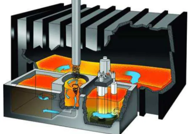
For over a decade, the Metaullics LOTUSS System has been the industry-leading technology for submerging light gage aluminum scrap in a standard reverberatory melting furnace. The LOTUSS System (Figure 1) has been effectively designed to provide rapid submergence of lightweight aluminum chips and turnings into molten aluminum, maximizing liquid metal yields and minimizing detrimental oxide formation. With dozens of international installations, LOTUSS Systems collectively recycle millions of tons of aluminum scrap annually.

In recent years increasing energy constraints have required continual improvements in overall furnace and melting efficiency, and with these stricter demands on energy reduction tighter controls on design characteristics must be implemented on all systems. Hence, advanced engineering tools are being employed to provide more accurate calculations relative to real-world applications.

One such engineering tool is computational fluid dynamics (CFD) simulations. CFD models have been used for many years on industrial applications such as process piping and casting/forming operations, but tremendous increases in computational “horsepower” have made full industrial process simulations faster and more user-friendly.

A series of CFD modeling trials were recently initiated to confirm if the submergence and circulation action within a LOTUSS System could be effectively modeled. The results of the computer models were compared to previous full-size physical water models to verify accuracy of the models.

Figure 1: Typical LOTUSS and circulation pump arrangement in an aluminum melting furnace

Model Equations

The CFD model solves differential equations describing the conservation of mass and momentum in order to evaluate the velocity and pressure in the LOTUSS system. The flow is driven by the incompressible Reynolds Averaged Navier-Stokes equations [1]: [( )( )] 0 T T p t ρ⎛_⎜∂ + ⋅ ∇ ⎞_⎟= −∇ + ∇ ⋅ μ μ+ ∇ + ∇ +ρ ∂ ⎝ ⎠ ∇ ⋅ = u u u u u g u (1)

where ρ, u, p, μ, g denote the density, the velocity, the pressure, the fluid viscosity and the gravity respectively.

The turbulent viscosity μ is computed using the standard kT − ε

model of turbulence [2]: 2 T μ k μ ρC ε = (2)

The turbulence kinetic energy k and its dissipation rate ε are obtained by solving the following transport equations:

( ) T T k k ρ k k P ε t μ μ μ ρ σ ⎡⎛ ⎞ ⎤ ∂ ⎛ _{+ ⋅ ∇} ⎞_{= ∇ ⋅ + ∇ + −} ⎢⎜ ⎟ ⎥ ⎜_∂ ⎟ _{⎜ ⎟} ⎝ u ⎠ ⎢⎣⎝ ⎠ ⎥⎦ u (3) ( ) 2 T εl T ε2 ε ε ε ε ρ ε ε C P C t k k μ μ μ ρ σ ⎡⎛ ⎞ ⎤ ∂ ⎛ _{+ ⋅ ∇ = ∇ ⋅}⎞ _{+ ∇ + −} ⎢⎜ ⎟ ⎥ ⎜_∂ ⎟ _{⎜ ⎟} ⎝ u ⎠ ⎢⎣⎝ ⎠ ⎥⎦ u (4)

where P( )u = ∇u:

(

)

1.44

εl

C = , Cε2=1.92, 0.09Cμ= . Turbulence equations are

solved for the logarithms of k and ε, thus increasing the accuracy and robustness of the solution algorithm [3].

Velocity boundary conditions are imposed on the inlet from the pump and on solid boundaries (walls):

( ) ( )( ) 0 pump pump T T w wall x on p on μ μ τ = Γ ⎫ + ∇ + ∇ ⋅ − = ⎪ _Γ ⎬ ⋅ = _⎪⎭ u u u n n u n U (5)

The wall shear stress τw as well as the turbulence boundary

conditions are given by a law of the wall model [1].

Free Surface Simulation

The scope of the present study was the solution of the free surface flow inside the LOTUSS System. Therefore, in addition to the equations describing the flow inside the computational domain, a numerical approach was introduced to be able to provide the location of the free surface. Two solution algorithms were considered in this work. The first one considered a simplified model in which the free surface inside the LOTUSS was maintained at the initial value by imposing a zero vertical velocity at the respective location. The CFD model then predicted a pressure build-up on the horizontal free surface that could easily be correlated with an equivalent free surface elevation by using the following relationship [4]:

(

)

This approach was very well suited to the case where the free surface exhibits small deformations, thus providing an easy correlation between the surface elevation and the flow dynamics. Because the pressure varies as 2

U

ρ it was obtained that the free surface elevation depends on the Froude number 2

( )

Fr=U / gL , where L is a characteristic length of the LOTUSS system.

The second solution algorithm considered the complete solution of the free surface problem by using a level-set method [1]. For this process a tracking function F was generated which indicated the position of the free surface: F is positive in the regions of the computational domain that are occupied by the liquid metal and negative in the empty regions. Once initialized to correspond to the starting location of the free surface, the tracking function was updated by solving the transport equation:

0 F F t ∂ _{+ ⋅ ∇ =} ∂ u (7)

The CFD model considered different material properties in the flow cells that were occupied respectively by the liquid metal and by the air. In the presence of gravity forces such an approach generated spurious oscillations in the proximity of the free surface because of the inconsistency between the discrete representations of the pressure and gravity forces. One way to improve the solution accuracy was to consider enriched pressure shape functions on elements containing the flow interface [5]. This finite element method produced a discontinuous gradient pressure field in agreement with the gravity force which was also discontinuous across the interface between the liquid metal and the air.

(a) Complete view

(b) Detail of LOTUSS system and mesh Figure 2: Computational domain for the LOTUSS system

Process Modeling

Using three-dimensional modeling software, a geometric representation of the desired 40” LOTUSS System [1-meter I.D.] was created, which included the flow channel from the pump, the internal LOTUSS bowl design, the discharge piping and an external reservoir. Figure 2 shows the computational domain which was analyzed. This domain was discretized using 4-node tetrahedral finite elements with a mesh containing 148,161 nodes and 846,839 elements (see Figure 2(b)). The external reservoir was included to provide the proper hydrostatic pressure in the system. In order to reproduce experimental conditions the analysis was performed using constant material properties corresponding to water at ambient temperature:

• density 3

1000 kg m/

ρ=

Simulations were carried out for an initial water level of 9” [229mm] above the discharge riser level and for pump flow rates of 600 GPM and 1000 GPM [2280 L/min and 3800 L/min, respectively]. For industrial relevance, these flow regimes correspond (respectively) to 360 and 600 tons/hr molten aluminum flow circulation.

Analysis of Numerical Results

Transient state computations were carried out to determine the position of the free surface. The vortex forms quite rapidly inside the LOTUSS System and the size of the vortex stabilizes after 15-20 seconds (which also correlates with field experience in molten aluminum).

(a) Velocity

(b) Pressure

Figure 3: Velocity and pressure distributions for 600 GPM pump flow rate

Figure 3 presents the velocity and pressure distribution in the LOTUSS system for the 600 GPM pump flow rate. The same results are shown in Figure 4 for the 1000 GPM pump flow rate. In both cases the enclosure is shown in transparency and a cut was made along a plane through the center of the enclosure. The velocity is higher at the external region of the LOTUSS enclosure, around the riser corners as well as at the inner curvature of the pipe where the flow is expected to be accelerated. The pressure is zero on the free surface and then increases with greater depth from the free surface.

(a) Velocity

(b) Pressure

Figure 4: Velocity and pressure distributions for 1000 GPM pump flow rate

Figure 5 shows the flow inside the LOTUSS System for the 600 GPM pump flow rate. The enclosure is shown in transparency in order to visualize the flow pattern. The position of the free surface is shown and the flow is illustrated by velocity vectors plotted on the free surface. The vortex shape can be clearly seen. Flow streamlines from points located within the flow from the pump are shown in Figure 5. The color of the streamlines is identified according to the flow integration time; blue indicates that the flow is just entering from the pump, whereas red indicates a longer flow path. Streamlines indicate that the flow from the pump induces a rapid central circulation which generates a strong vortex action, promoting aggressive scrap submergence from the free surface.

Figure 5: Flow pattern at 600 GPM flow rate

Similar results are observed in Figure 6 for the 1000 GPM pump flow rate. The vortex center is much deeper in this case and the outer vortex is higher when compared with the lower flow rate case. The streamlines from points located in the flow from the pump indicate that the flow from this region is rapidly entrained into the exit pipe.

Figure 6: Flow pattern at 1000 GPM flow rate

In order to simulate the possible submergence action of the induced vortex, tracer locations were originated near the free surface and allowed to circulate unrestrained within the LOTUSS. The path of these tracer particles indicates the probable route traveled by a particle (i.e. scrap aluminum chip) placed within the envelope of the vortex cone. As portrayed in Figure 7 (at 1000 GPM flow rate), particles placed closer to the center of the vortex are likely to submerge quicker, whereas particles at the outer edge will recirculate indefinitely on or near the surface of the free vortex. In the future, expansion of this computational model to incorporate thermodynamics and melting reactions may facilitate a complete scrap recovery simulation.

(Close to Center)

(Near Outer Edge)

Figure 7: Circulation path of tracer particles placed on the vortex surface (1000 GPM flow rate)

Next, the geometric vortex parameters of the computational model were plotted to facilitate comparison with previous physical water modeling of a full-size LOTUSS System. As shown in Figure 8, the shape of the vortex of each flow condition is plotted, showing the width of the vortex relative to the vertical position above the discharge riser. It should be noted that the initial bath level (reservoir level) was 9” [229mm] above the riser. The solution for the 600 GPM pump flow rate (shown in red) displays a flatter vortex than the one at 1000 GPM (shown in blue). When solving for the higher flow rate, the center of the vortex (i.e. the apex) penetrates much deeper towards the discharge riser creating a region which is relatively unstable where air is entrained into the outflow. In order to determine the position of the apex of the vortex cone, an estimation was taken of the locations where the width of the vortex equal the element size and twice the element size, respectively. Those two locations are indicated by discontinuous lines in Figure 8.

Figure 8: 40” LOTUSS: Vortex geometry above discharge riser

The numerical results for the size and position of the vortex cone are also compared with experimental data from the previous physical water model. Figure 9 presents the vortex height above bath, which represents the highest position of the vortex cone (along the sidewall) with respect to the initial bath level (9” above riser). The experimental data is shown by the black diamond symbols, whereas the blue and red symbols are from the numerical solution: the red squares indicate the prediction of the simplified small perturbations model and the blue circles are from the complete free surface model. The quadratic approximation that passes through the simplified model prediction at 600 GPM pump flow rate is also shown with a red discontinuous line. As can be seen both models are accurate, as well as the quadratic approximation.

Figure 9: 40” LOTUSS: Vortex height above bath

The results for the total vortex height (i.e. vertical distance from sidewall to apex) are compared in Figure 10. Here again the experimental data are compared with predictions from the two models and to the quadratic approximation of the simplified model solution. For the total vortex height, the simplified model underestimates the measured value by about 30%, whereas the prediction from the free surface model is much closer to the experimental value. However, due to the “violent” nature of the high velocity fluid flow, physical measurements of the experimental model may have +/- 10% variability. For the higher pump flow rate an interval was plotted as determined by the locations where the width at the apex of the vortex equals one and respective two mesh element size (i.e. vortex cone was nearly vertical). Overall, for an initial simulation with limited data, the free surface solution provided an accurate starting point for future models.

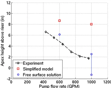
Finally, Figure 11 presents the results for the position of the apex (depth) of the vortex cone with respect to the riser level. In this case the prediction from the simplified model is not sufficiently accurate. However, it is clear that the free surface model is able to accurately predict the apex of the vortex cone.

For the 1000 GPM pump flow rate the numerical prediction is again given in the form of an interval. For this case, the free surface of the vortex is almost vertical on a relatively large region around the apex. This response indicates that air is probably entrained in the outflow by the collapse of small portions of the free surface. Furthermore, it should be noted that in the vicinity of the apex of the vortex cone there are clearly large deformations of the free surface from the initial horizontal position. The results in the Figures 10 and 11 illustrate the limitations of the simplified approach when the free surface exhibits large deformations.

Figure 11: 40” LOTUSS: Apex height above riser

These results verify that the complete free surface model is more accurate and compares very well with the measured experimental values. However, the simplified model may provide useful correlations that can take into account the size of the LOTUSS system and the pump flow rate.

As identified herein, the computational fluid dynamic modeling of the Metaullics LOTUSS System provided an effective representation of real-world molten aluminum circulation scenarios. This simulation system may be implemented immediately as a practical tool for predicting the free surface geometry of a submergence vortex prior to initiating refractory/furnace construction. As additional modeling projects are performed in the future, subsequent data points and statistical analysis will create enhanced accuracy in the overall model.

Conclusions

• It is expected the vortex height to vary according to the square of the inflow velocity and the inverse of the enclosure diameter.

• The computational model provides a valid representation of the flow inside the LOTUSS System and presents a useful tool for visualizing the circulation action.

• The path of tracer particles placed on the vortex surface may offer an indication of the possible submergence efficiency of the system without the immediate need for complicated thermodynamics calculations.

• Both the simplified model and the complete free surface model can accurately predict the vortex height above bath. The position of the apex of the vortex cone is much more difficult to predict, and only the free surface model provides accurate solutions within 10% variation from experimental values.

• The region around the apex of the vortex cone presents a very abrupt descent in the case of the 1000 GPM pump flow rate. As was observed in the simulation, free surfaces of the vortex boundary are very close to each other with a significant curvature that would lead to free surface breakdown; it is expected that air would be entrained by the flow into the exit pipe.

• Overall, these preliminary trials verified the accuracy and efficiency of utilizing free surface computational modeling to perform simulations on the Metaullics LOTUSS System.

References

[1] F. Ilinca, J.-F. Hétu, “Finite Element Solution of Three-Dimensional Turbulent Flows Applied to Mold-Filling Problems,” Int. J. for Numerical Methods in Fluids, 2000; 34: 729-750. [2] B.E. Launder and D.B. Spalding, Mathematical Models of Turbulence, 6th ed., Academic Press, London, 1972.

[3] F. Ilinca and D. Pelletier, “Positivity Preservation and Adaptive Solution of the k-ε Model of Turbulence,” AIAA Journal, 1998; 36(1): 44-50.

[4] M. Piva and E. Meiburg, “Steady axisymmetric flow in an open cylindrical container with a partially rotating bottom wall,” Physics of Fluids, 2005; 17.

[5] A.H. Coppola-Owen and R. Codina, “Improving Eulerian two-phase flow finite element approximation with discontinuous gradient shape functions,” Int. J. Num. Methods Fluids, 2005: 49: 1287–1304.