Analysis of the Los Angeles metropolitan office market

Analysis of the Los Angeles Metropolitan Office Market

by

Norito Makimoto Bachelor of Law Sophia University, Tokyo

1987

Submitted to the Department of Urban Studies and Planning in Partial Fulfillment of the Requirements for the Degree of

MASTER OF SCIENCE in Real Estate Development

at the

Massachusetts Institute of Technology September 1995

@1995 Norito Makimoto All rights reserved

The author hereby grants to MIT permission to reproduce and to distribute publicly paper and electronic copies of this

thesis document in whole or in part.

Signature of the Author

Norito Makimoto Department of Urban Studies and Planning August 11, 1995

Certified by _AWilliam

C. Wheaton

Professor of Economics and Urban Studies and Planning Thesis Supervisor

Accepted by ' .-

-William C. Wheaton Chairman Interdepartmental Degree Program in Real Estate Development

iAACHUSETTS INSTriTE OF TECHNOLOGY

SEP 2 8 1995

Analysis of the Los Angeles Metropolitan Office Market

by

Norito Makimoto

Submitted to the department of Urban Studies and Planning in Partial Fulfillment of the Requirements for the Degree of Master of Science in Real Estate Development

at the Massachusetts Institute of Technology

Abstract

The thesis predicts the future of the Los Angeles metropolitan office market through analysis of the office decentralization in the area, particularly facts and causes. We first look at the real estate data for 43 submarkets in the metro area Through studies of the area's office market, the long term trend of the decentralization was observed. As Los Angeles County declined in share of employment and office stock, other regions grew continuously over the years.

As causes of the decentralization, we focus on wage differentials and commuting time of each subcenter. Estimated wage premia and average commuting time are found to vary significantly over the subcenters. Also positive and significant correlation is found between wages and commuting time, as urban economic theory predicted. Therefore, there is an incentive for firms to move out to the locations with shorter commuting time.

Comparing real estate data directly to average commuting time and estimated wage premia, we estimate relationships between facts and causes. Two equations are adapted to this estimate for scale and growth of subcenters. As a result, larger subcenters are found to have longer commuting time and higher wage premia; shorter commuting time and lower wage premia cause faster growth of subcenters. Thus, smaller subcenters with shorter commuting time and lower wage premia are proved to have a potential for future growth.

Finally, we forecast future vacancy rates and rents of each subcenter. Most of the badly performing subcenters are located in Los Angeles County, whereas the well

performing subcenters are located in peripheral counties. In addition, the total score calculated for each subcenter tells us that the central locations will decline further in future, whereas subcenters at the fringe locations will grow. Therefore, we concluded there is less hope for office markets in the central locations.

Thesis Supervisor: William C. Wheaton

Acknowledgment

I would like to thank the following people for their generous assistant and input in

my completing this thesis;

My advisor, Professor William C. Wheaton, who had provide me with precious

advise and idea throughout the thesis writing process and also accepted me to use the data from his research company.

Mr. Darren Timothy, a doctor student of the Department of Economics, who originally developed the approach of estimating wage premia, which we used in this thesis, and instructed his methodology very kindly to me.

Mr. John A. Southard and Ms. Laura Stone from CB Commercial/Torto Wheaton Research, who helped estimation from the data and also gave me a lot of advises.

TABLE OF CONTENTS

1. INTRODUCTION AND THESIS OUTLINE ... 7

1.1. INTRODUCTION...

7

1.2. THESIS OUTLINE ... 8

2. HISTORY OF THE LOS ANGELES OFFICE MARKET... 10

2.1. THE Los ANGELES METROPOLITAN AREA... 10

2.1.1. Overview...10

2.1.2. Area Definition ... 12

2.1.3. Long Term Trends of Subcenters' Office Stock...14

2.2. LONG TERm TRENDS IN OFFICE EMPLOYMENT ... 14

2.3. RECENT TRENDS OF THE OFFICE MARKETs ... ... 15

2.4. REGIONAL M ARKETS ...--.-... ... 19

2.4.1. Los Angeles County ... 19

2.4.2. Orange County ...-- 21

2.4.3. Oxnard...22

2.4.4. Riverside County/San Bernardino County...24

2.5. CONCLUSION... 26

3. TRAVEL TIME AND ESTIMATION OF WAGE DIFFERENTIALS .... 27

3.1. INTRODUCTION...27

3.3. PREVIOUS RESEARCHES ... 31

3.4. D ATA ... ..- 34

3.4.1. Census Micro Data...34

3.4.2. Public Use Microdata Area...34

3.5. TRAVEL TIME...36

3.6. ESTIMATED WAGE EQUATIONS... 38

3.6.1. Individual Characteristics ... 38

3.6.2. Wage Premia...40

3.7. TRAVEL TIME AND WAGE DIFFERENTIALS...46

3.8. CONCLUSION...48

4. OFFICE DECENTRALIZATION, WAGES AND TRAVEL TIME... 49

4.1. INTRODUCTION... ...- 49

4.2. SCALE OF SUBCENTERS, AND TRAVEL TIME AND WAGE PREMIA ... 50

4.2.1. Equations...50

4.2.2. Results of Estimates ... 51

4.2.3. Comparison: Actual and Predicted ... 53

4.2.4. Findings...54

4.3. GROWTH OF SUBCENTERS, AND TRAVEL TIME AND WAGE PREMIA ... ... 55

4.3.1. Equations...-56

4.3.2. Results of Estimates ... 56

4.3.3. Analysis of the Past Growth: Actual and Predicted ... 58

5. FORECASTING OFFICE SUBMARKET GROWTH... 61

5.1. VACANCY RATE FORECASTS...61

5.2. R ENT FORECASTS... .64

5.3. FINDINGS ... 66

6. CONCLUSION... 69

6.1. SCORE MATRIX...70

6.2. RESULTS FROM THE SCORE M ATRIX ...- 70

1. Introduction and Thesis Outline

1.1. Introduction

Over the past decade the decentralization of office firms from major metropolitan areas in the US has been a common phenomenon. While many American cities still contain large central business districts with numerous high-rise office buildings, office construction activities outside of the central business districts (CBDs) have increased dramatically since

1988. For example, Boston's share of regional jobs in finance, insurance and real estate

(FIRE), and service sectors dropped 12 percentage points from 47% to 37%, while shares of numerous suburban communities rose (DiPasquale & Wheaton 1995).

This current of decentralization caused the CBD market's decline and the suburban location's rise to prosperity in most metropolitan areas. Moreover, the recent property recession spurred this downward trend of the CBD office markets. Office buildings with huge vacant space left are familiar scenes in the central locations nowadays. There seems to be no more bright future in the CBDs, whose skyscrapers once were symbols of American prosperity, but now are becoming real white elephants. Is this really true? Is there really no hope for the CBD office markets?

The object of this thesis is to predict the future of the Los Angeles office market, through analysis of the decentralization in the Los Angeles metropolitan area, particularly facts and causes. Through a study of the office market history, facts of decentralization in the area are first observed. We next examine wages and travel time of workers in various locations of the area. Urban economic theory concluded that wage differentials over subcenters result in decentralization of office locations, and wages are related to travel time in the same location. Thus, estimations of relationships between wages and travel time tell us the trend of decentralization in the area. Finally, by forecasting future office markets,

we not only answer the question, but also suggest what the US metropolitan areas will be like in the future.

1.2. Thesis Outline

The thesis is organized as follows.

Chapter 2 analyzes the history of the Los Angeles metropolitan office market, using the CB Commercial data for 43 submarkets in the area. We explain each county's office market as well as the whole metropolitan area. The long term trends of the area clearly

suggest decentralization of its employment and office stock, although the downtown market still keeps stable share of area's office absorption. Prior to 1987 the area was characterized

by widely differing vacancy rates. But more recently vacancy rates have converged to

more equivalent rates.

Chapter 3 focuses on causes of decentralization, particularly travel time of workers and wage differentials. The approach developed by Darren Timothy is employed. Using the microdata from the 1980 Census and the 1990 Census, average travel time and wage premia of each work location are calculated. The results show travel time and wage premia

vary significantly across work locations of the metropolitan area. Also, there are significant positive correlation between travel time and wage premia.

Chapter 4 estimates relationships between facts and causes of decentralization. Real estate data from the CB Commercial are directly compared with average travel time and estimated wage premia from Chapter 3. Two equations are adapted in order to estimate these relationships in terms of scale and growth of subcenters. The results support urban economic theory; larger subcenters have longer travel time and higher wage premia, and

shorter travel time and smaller wage premia cause faster growth of subcenters.

Chapter 5 forecasts vacancy rate and rents of each subcenter in the metropolitan area during 6 years from 1995 to 2000, using equations estimated in Chapter 4. Los Angeles

County shows the worst performance in terms of both forecasted vacancy rates and

forecasted rents. On the other hand, two of the best performers in terms of vacancy rate is located at Orange County and all of the best performers in terns of future rents are located at either Riverside County or San Bernardino County.

Finally, Chapter 6 concludes the thesis with a summary of the results and findings. The best subcenter and the worst subcenter for investments are presented.

Finally, Chapter 6 concluded the thesis with a summary of the results and findings. The best and the worst subcenters are presented.

2. History of the Los Angeles Office Market

2.1. The Los Angeles Metropolitan Area

2.1.1. Overview

The Los Angeles metropolitan area is ranked as the second largest metropolitan area in the United States, with a population of 14.5 million people' (Bureau of Census 1994). The metropolitan consists of five counties: Los Angeles County, Orange County, Ventura County, Riverside County and San Bernardino County, these counties have a total office employment of 1,123 million people and 238 million square feet of office stock. In the past, the area's unemployment rate was quoted at 10.3% in the third quarter of 1994,

significantly higher than the national unemployment figure of 6.1% (Cushman & Wakefield 1994). Recent quakes, riots and floods plunged the area's fiscal management into harsh conditions. Los Angeles County is suffering from a 1.2 billion dollar budget gap and considering a plan to slash more than 18,000 jobs, 20% of the country work-force (Schine

1995). In the early 1995, Orange County filed for bankruptcy because of failure in

speculative investments. These fiscal problems in the area raise speculations of increasing property tax in near future.

After the property crash of the early 1990s, the office property market in the metropolitan area plunged into recession. In 1991, the area recorded the highest vacancy rate of 21.3%, according to CB Commercial data; this rate is approximately 4% higher than the average of previous five years. Thereafter, the rate has gradually decreased up to

19.5% in 1994, which is slightly smaller than 19.7% in 1993.

Figure 2.1 compares office stock and the annual completion of space as a

percentage of stock in the area. Completion of new office space is not always linked to the

U. S. macro-economy. Completion dropped sharply just after the recession of 1975 and 1990, but continued to rise through the downturns in the early 1980s. This unique

outcome in the early 1980s can be explained by the policy implemented by the Reagan administration. Deregulation of financial institutions had created excess funds available for new investments and the 1981 tax reform had fueled investments in the property market. Figure 2.1 also shows that, in the Los Angeles metropolitan area, the building boom in the

1980s was much smaller than the earlier boom from the late 1960s to early 1970s when measured as a percentage of the existing stock. This implies that the area's office market has matured through the early 1980s; a rapid growth in this area would not be expected

thereafter.

Figure 2.1: Total Stock & Completion as a Percentage of Stock in the LA Metropolitan Area

250- 18.0 16.0 2 0 0 - - - -- - --- - - - - - - --- ---- --- - 14 .0 12.0 6 o 150 -10.0 c 8.0 -" 500 -100 --6.0 0 50--2.0 0 -- 0.0 CD CO r- r__ r. r- I~- Go 00 CO 00 00 CD C Year EM Stock -O-Comp.(%)

2.1.2. Area Definition

"Los Angeles" has three different conceptual meanings:

1) The Los Angeles metropolitan area2

2) Los Angeles County

3) Los Angeles City

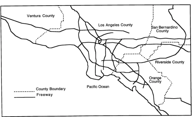
The Los Angeles metropolitan area is shown in Figure 2.2. In this paper, the Los Angeles metropolitan area is used for identifying the Los Angeles office market. This metropolitan area consists of four large regions: Los Angeles County, Orange County, Oxnard (Ventura County), and Riverside County/San Bernardino County, according to the

Figure 2.2: Los Angeles Metropolitan Area

2 In real estate terms, the greater Los Angeles includes four metropolitan statistical areas (MSAs) in

Southern California: the Anaheim-Santa Ana MSA, the Los Angeles-Long Beach MSA, the Oxnard-Ventura MSA and the Riverside-San Bernardino MSA (Crubb & Ellis. 1993).

CB Commercial data. Giuliano & Small (1991) distinguished 32 employment subcenters in the metropolitan area, adapting their empirical criteria for identification. We, however, define this metropolitan area with 43 office submarkets, as shown in Table 2.1, using the data from a real estate brokerage firm, CB Commercial. Since the purpose of this chapter is to analyze the office market, the firm's definition of the area could be more suitable for this purpose3_.

Table 2.1: Office Submarkets & Changes in Their Shares of Stock

SUBMARKETS

Los Angeles Co

Beverly Hills Beverly Hills Triangle Brentwood Corridor Burbank/N. Hollywood Century City

Cerritos Covina/Pomona East Los Angeles

El Monte/Baladwin Pk Fox Hills Hollywood LA Downtown LA Suburban LAX/El Segundo La Puente/Vlly Blvd. Long Beach Marina Del Rey Mid-Wilshire Miracle Mile

N San Fernando Vlly

Olympic Corridor Park Mile Pasadena/Glendale Santa Monica

Sherman OaksNn Nuys Thous Oaks/W'lake Vg STOCK (1000sf) 1974 2277 1785 440 328 3930 779 206 0 682 39 2330 15802 273 2546 0 1614 711 7919 2830 88 60 828 3318 503 2373 Share 3.4% 2.7% 0.7% 0.5% 6.0% 1.2% 0.3% 0.0% 1.0% 0.1% 3.5% 23.9% 0.4% 3.9% 0.0% 2.4% 1.1% 12.0% 4.3% 0.1% 0.1% 1.3% 5.0% 0.8% 3.6% 1994 3483 2574 3294 6116 8507 3611 2971 936 3690 2534 2646 35862 525 11021 1491 7738 1195 9033 4590 1904 1796 1293 13698 6281 8351 Share 1.5% 1.1% 1.4% 2.6% 3.6% 1.5% 1.2% 0.4% 1.5% 1.1% 1.1% 15.0% 0.2% 4.6% 0.6% 3.2% 0.5% 3.8% 1.9% 0.8% 0.8% 0.5% 5.7% 2.6% 3.5% 491 0.7% 1340 0.6% SUBMARKETS Torrance/Carson Warner Ctr/W Vlly West Hollywood West Los Angeles Westwood STOCK (1000sf) 1974 Share 388 0.6% 1251 1.9% 912 1.4% 190 0.3% 1801 2.7% 1994 6893 9078 1121 3032 3168 Share 2.9% 3.8% 0.5% 1.3% 1.3% Total 56694 85.8% 169772 71.2% Orange Co Coastal/ Airport 2699 4.1% 25581 10.7% Ctrl Orange Co 3382 5.1% 12469 5.2% North Orange Co 540 0.8% 4099 1.7% South Orange Co 181 0.3% 4247 1.8% West Orange Co 180 0.3% 3022 1.3% Total 6982 10.6% 49418 20.7% Oxnard Camarillo 75 0.1% 686 0.3% Conejo Valley 193 0.3% 2504 1.1% Oxnard/Pt Hueneme 267 0.4% 1015 0.4% Ventura County 518 0.8% 1827 0.8% Total 1053 1.6% 6032 2.5% Riverside/San Bernardino Co East Valley 441 0.7% 3708 1.6% Pomona Valley 45 0.1% 4084 1.7% Riverside 831 1.3% 5300 2.2% Total 1317 2.0% 13092 5.5%

LA Metro Area Total 66046 100% 238314 100%

Source: CB Commercial/Torto Wheaton Research

3 The Los Angeles metropolitan area is defined with 28 work locations in the Public Use Microdata. We

use this area definition to estimate wage differentials and average travel time in the Chapter 3. In the Chapter 4, we merge 43 office submarkets into 28 in order to fit the Census definition.

2.1.3. Long Term Trends of Subcenters' Office Stock

Total office stock of the area is approximately 238 million square feet in 1994 according to the CB Commercial data. Table 2.1 also shows office stock of each submarket and its share of the metropolitan area both in 1974 and 1994. Bold indicates growth of share in 1994 compared to the share in 1974. Los Angeles County alone decreased its share in the metropolitan area; 13 of its 30 submarkets lost their share since

1974. Particularly the center markets, the downtown and Mid-Wilshire Corridor, declined significantly. In contrast, most of submarkets in the other three regions raised their presence in the area, with an exception of West Orange County.

2.2. Long Term Trends in Office Employment

Decentralization can also be seen by examining the government produced employment data. Figure 2.3 presents changes in total office employment in the

metropolitan area and percentage share of each county of the area during 28 years. Total office employment in the metropolitan area peaked in 1990 at the level of 1,145 thousand office workers. This number had grown rapidly and consistently without a major slump from 424 thousand in 1967; the average annual growth rate of these 28 years was

approximately 4.7%. However, the total figure has hit a plateau these past four years and never come back to the level in 1990.

Figure 2.3: Total Office Employment in the LA Metropolitan Area & Share of Each Region

1200 - - 90 08 -- -00 1 0 0 0 - - -- - - --- --- - - --- --- - ---- - -- -- -- - --- --- ---- - -70 C 00 8 0 0 -- -- - - -- ---- - -- ---- --- --- - . - --- 6 0 E 050 0 600 - --- - - --- --- -- ---0- 40 E W e 400 - - ---- 30 a 0 20 200 - - - - - - - -- x -- - -10 0 10 Year -z-

-Total Em-p. - Los Angeles " Orange I& Qxnard ---- Riverside/San Bernardino

Source: CB Commercial/Torto Wheaton Research

It is also clear from Figure 2.3 that decentralization has been a long term trend in the metropolitan area from the early stage. Los Angeles decreased its share in the area's office employment to 65.3% in 1994 from 82.9% in 1967. On the other hand, although the other three regions gained their shares together in this period, Orange County has grown most rapidly by 12.4 points in its share from 9.8% to 22.2%; its average annual growth rate in these 28 years was approximately 8%.

2.3. Recent Trends of the Office Markets

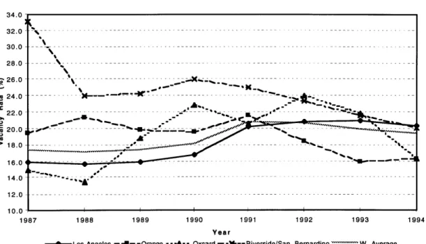
The weighted average vacancy rate in the area has been stable within the range from

17 to 21% since 1987, as shown in Figure 2.4. In the three markets, Los Angeles County,

Orange County and Oxnard, vacancy rates have moved closely together since 1987. Riverside County/San Bernardino County, on the other hand, has consistently shown

Figure2.4: Average Vacancy Rate of Each Region 34.0-32.0 -30.0 28.0 -26.0 : : 22.0 >18.0 16.0 12.0 1987 1988 1989 1990 1991 1992 1993 1994 Year

-- -- Los Angeles - - --Orange - --A-- Oxnard - ---- Riverside/San Bernardino --- W. Average

Source: CB Commercial/Torto Wheaton Research

higher rate than each of the other three markets until 1992, particularly 15.7% higher than the weighted average rate in 1987. Currently, however, data shows that all four markets are in the smallest range of 4% in 1994. This may suggest that the Riverside County/San Bernardino County office market had been independent from the metropolitan market until

1992, but has

joined

Figure 2.54 represents each county's share of net absorption in the area's office market. In 1994, Orange County was a big looser with negative net absorption, whereas the other three regions increased their shares, particularly Oxnard, whose share increased to

29.0% from 4.2%. The Oxnard market, only 2.5% of the area's stock, absorbed a

4 In the data from CB Commercial, vacancy rate of each market is available only from 1987. In order to

calculate the average absorption between 1974 and 1987, we first assumed the vacancy rate of the Los Angeles in 1974, 15.3%, as each submarket's vacancy rate in 1974, since vacancy rate in Los Angeles County is available even during 1974 and 1987. Then, we calculated the average absorption in 13 years from 1974 to 1987 by following equation:

(stock in 1987 x vacancy rate in 1987 - stock in 1974 x 15.3%) / 13 years

This calculation was used for all average numbers during 1974 and 1987 in following graphs of this chapter.

significant amount of space in 1994. Similarly, in the early 1990s, Los Angeles County lost its share of absorption by more than 40 points from the over 60% level in 1990.

Figure2.5: Each Region's Share in Net Absorption

70.0 60.0 50.0 0 40.0 S00 Z, 30.0 - - - - - - -- - - - - - - -- - - - - - - ---- - -o - - - - - -e 20.0 0 0 0 0 _A. X ... -10.0 1974-87 1988 1989 1990 1991 1992 1993 1994 Year

- Los Angeles - 4--Orange - -- --Oxnard - ---- Riverside/San Bernardino

Source: CB Commercial/Torto Wheaton Research

Over the long term, Los Angeles County has lost its share of absorption; it had only

50% share in 1994, although once it had dominated the metropolitan market with an

average share of 70% during the period from 1974 to 1987. The other three regions

(Orange, Oxnard and Riverside/San Bernardino) have grown their market. Particularly, the two peripheral regions, Oxnard and Riverside County/San Bernardino County, have

increased their share enormously up to 29% and 22% respectively in 1994, from their average shares between 1974 and 1987, 4.3% and 3.5%. Orange County also has grown its share rapidly above the 40% level in recent years, which was nearly doubled from the

average share of 24% in the previous 8 years, although the county experienced a strong downward movement in 1994. As a result, the difference of shares among the four regions has been diminished in terms of net absorption.

Figure 2.6: Average Asking Rent of Each Region 22.0 21.0 20.0 19.0 -18.0---A... $ 17.0 .C 16.0 15.0 14.0 13.0 1987 1988 1989 1990 1991 1992 1993 1994 Year

-4---Los Angeles --- Orange ---A-- Oxnard ---- Riverside/San Bernardino-W. Average

Source: CB Commercial/Torto Wheaton Research

Average asking rents in the four markets have decreased continuously and constantly since 1991 by approximately $1 per square foot per year. In addition, those markets have been very well correlated with each other since then. The difference between the highest rent, Orange County, and the lowest, Riverside County/San Bernardino

County, is $3.5 per square foot in 1994 (Figure 2.6). This dollar difference is clearly smaller than that in 1987, which was $5.8 per square foot. Therefore, we could say there was a convergence in the office rent level in the area's market in the early 1990s.

2.4. Regional Markets

2.4.1. Los Angeles County

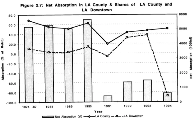
Los Angeles County contains the greatest number of office submarkets in the entire metropolitan area, with 71.2% of the area's total office stock. Downtown LA alone

comprised 15% in 1994. Over the long term, the county has diminished its presence. Figure 2.7 shows that its share of net absorption in the metropolitan area decreased to the

50% level in 1994 from the average between 1974 to 1987, 68.4%. The downtown

market, however, has kept its share stable, with an exception of extreme large negative absorption in 1994. As a result, other submarkets in the county declined in share of absorption particularly during the past several years.

Figure 2.7: Net Absorption in LA County & Shares of LA County and LA Downtown 80.0 . 6000 60.0 - - - --- -5000 40.0 -0.0 ---- -- - 3000--

--

---20

.0-

--

C:===Net Absorption (sf) -- -LA County -- 4I- - LA Downtown

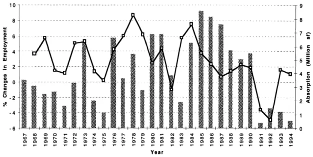
Figure 2.8: Office Employment and Absorption in LA County 9 8 7. 6 5j 4 C 0. 3 -0 .0 2 < 1 0 r- CO mc 0 CI j c M 0t CO I- CO 0) m . No MCo0 co r- Co mc .- oj N Mo (D C Co D r- - - - r- t'- t~ 1- t- t- CD GO CO Co CO Co CO Co CO Co m) m m IM m0 Year

mm Absorption (Million sf) -D-% Change in Employment Source: CB Commercial/Torto Wheaton Research

Figure 2.8 compares annual office employment growth with the annual net

absorption of office space in Los Angeles County. It is observed that office employment in Los Angeles County has reacted sensitively to the national economy, experiencing

significant downturns near the national recessions in 1971, 1975, 1982, and 1992. Figure

2.8 also suggests that net absorption in Los Angeles County is significantly correlated with

its office employment growth. The changes in office employment during the 1970s and 1980s were relatively constant, however, the county's net absorption during the 1980s was much larger than that in the 1970s. One explanation is that the total employment in the

1980s was greater than the 1970s. Another possible explanation for this is that during the 1980s each employee used more space than during the 1970s.

2.4.2. Orange County

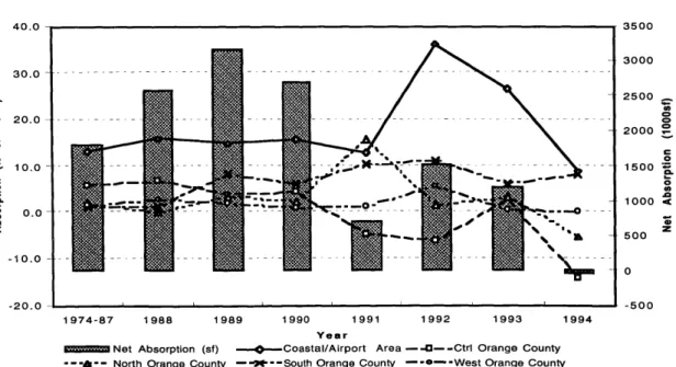
Figure 2.9 shows total net absorption and each submarket's share of the metro area's net absorption in Orange County. As a long term trend, Coastal/Airport Area, the biggest submarket in the region, has grown farther with higher share of net absorption in the area particularly in 1992 and 1993, 36.2% and 26.5% accordingly. In contrast, Central Orange County, which once had the second highest average share of net absorption in the period from 1974 to 1987 has declined, experiencing negative net absorption in 1991, 1992 and 1994. The other three submarkets have grown gradually with a few exceptions for each submarket, especially in 1994.

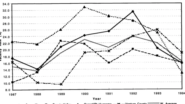
Recently, particularly after the property crash in the early 1990s, vacancy rates in the region have converged at the lower level with an exception of Central Orange County, as show in Figure 2.10. The difference between the highest vacancy rate and the lowest in the region dropped to 4.4 points in 1992 from the largest level of 20.6 points in 1988, as

Figure 2.9: Net Absorption & Each Submarket's Share in Orange County 40.0 - 3500 3000 30.0 -- 2500 2 0 .- - - -- - - ". - - - s - - - - - - - - - --- - -- - - - - - - - - -- --- -- C ) S- .-- 2000

2

Net Absorption (sf) ---- Coastal/Airport Area -- O--Ctr Orange County

-- North Orange County - -M--South Orange County ---- West Orange County

the average vacancy rate in the region decreased. This lowering vacancy rate and

convergence of the vacancy rates in the region are mainly due to the limited amount of new supply coming into the market. The submarkets in the region had new completion of only

216,000 square feet in the past three years.

Figure 2.10: Vacancy Rate of Each Submarket in Orange County

32.0 -30.0 28.0-26.0 24.0- 22.0-o 20.0-10 18.0 16.0 14.0- 12.0-10.0 -1987 1988 1989 1990 1991 1992 1993 1994 Year

-.--- Coastal/Airport Area - -U- -Ctrt Orange County ---A-- North Orange County

- -X--- South Orange County - -6--West Orange County W. Average

Source: CB Commercial/Torto Wheaton Research

2.4.3. Oxnard

The Oxnard office market appeared to be extremely volatile in Figure 2.11, with a considerably small stock of 6 million square feet, showing the lowest net absorption of

-170,000 square feet in 1992, and the highest of 333,000 square feet in 1994.

Consequently, submarkets in the region show unsteady movements, largely due to their limited size of office stock. Over the long term, however, most submarkets in the region have increased their shares of net absorption in the metropolitan area. For example, these four submarkets had the average shares of only 0.4 to 1.7% in the period from 1974 to

Figure2.1 1: Net Absorption & Each Submarket's Share In Oxnard 10.0 12.0- -soo 1 0 . 0 - - - - -- - - -- - - - - - - - -- - -- ---- - -- - - - ---- - - -- - - - - - - -- 300 6 .o -- -- - - - - -- -8.00 - -- - --- -- - - - - - - - - - - - - - - -- - - - - -6.0 - - - --- - -- - --2 .0 - - - -- - - - --- ---- --- ---- -- -1- -0-4.0 9 19 1 0 0.0 f . -100 - 2 . 0 - - - - - - - - - - - - - - - - - - - - - - - - - -- - - - - - - - --4.0 1 i i ii 1-200 1974-87 1988 1989 1990 1991 1992 1993 1994 Year

Net Absorption (sf) ---- Camarillo -- 0--Conejo Valley --- s-- Oxnard/Pt Hueneme - -X- --Ventura County

Source: CB Commercial/Torto Wheaton Research

1987, but in 1994 Oxnard/Port Hueneme and Ventura County recorded over 10% shares

of absorption.

Similar to the changes in shares of net absorption, vacancy rates of the region's submarkets moved widely. Camarillo with only 600,000 square foot stock, for example, varied its vacancy rate from the lowest, 14.2% in 1988, to the highest, 31.5% in 1991, as shown in Figure 2.12. Similarly Oxnard/ Port Hueneme had 1,015,000 square foot stock, whose vacancy rates ranged from the highest of 32.9% in 1992 to the lowest of 12.9% in

1994. However, although each market in the region has been volatile, the region as a whole has been smoothed since 1991. In 1990, for example, there was 13.8% difference between the highest vacancy rate and the lowest in the region. In contrast, in 1994, this difference was only 6.1%.

Figure 2.12: Vacancy Rate of Each Submarket in Oxnard 34.0 32.0 - ---- ---- - - - - --30.0 -28.0 26.0 24.0 22.0 -o 2 0 .0 -e 018.0 10.0 1 4 . - - - - - - -- - -- - - - - - -12.0o - --- - - - -- - - - -1' 0.0 -- - --- - -- -- -1.0 1987 1988 1989 1990 1991 1992 1993 1994 Year

--- 4--Camarillo - --- -Conejo Valley --- Oxnard/Pt Hueneme - -- -- Ventura County -W. Average

Source: GB Commercial/Torto Wheaton Research

2.4.4. Riverside County/San Bernardino County

Riverside County/San Bernardino County is a rather new market and has existing office stock of 13 million square feet, representing 5.5% of the area's stock. This region had over 1.5 million square foot net absorption in 1988 and 1989, which is more than three times bigger than the average net absorption between 1974 and 1987 (Figure 2.13).

Submarkets in the region also have a long term trend of increasing their shares of net absorption in the metropolitan area. Over the period from 1974 to 1987, the existed three submarkets had average shares of only 1.0 to 1.6%. However, most submarkets recorded higher shares in the past seven years, except in 1992 and 1993. As a short term trend, Riverside has grown rapidly, particularly in 1994, gaining a 17.4% share. In contrast, East Valley declined with negative absorption in 1992 and 1993.

Figure 2.13: Net Absorption & Each Submarket's Share in Riverside County/San Bernardino County

1974-87 1988 1989 1990 1991 1992 1993 1994

Year ..

E Net Absorption (sf) 0 East Valley --- Pomona Valley I&-Riverside

Source: CB Commercial/Torto Wheaton Research

Figure 2.14: Vacancy Rate of Each Submarket in Riverside County/San Bernardino County

42.0 -40.0 38.0 -Y 36.0 -34.0 32.0 30.0 28.0 26.0 C 24.0 -22.0 -20.0 18.0 -16.0 -14.0 12.0 -10.0 -1987 1988 1989 1990 1991 1992 1993 Year

- East Valley - --- Pomona Valley ----- Riverside/San Bernardino W. Average

Source: CB Commercial / Torto Wheaton Research 20.0 15.0 10.0 0 5.0 1600 1400 1200 C 1000 C 0 600 0 400 200 0 1994

The region once suffered from extremely high vacancy rates, especially in 1987; Riverside experienced 40.3% vacancy rate in that year, as shown in Figure 2.14. After

1990, however, the average vacancy rate has decreased gradually to 20.4% in 1994, close

to the area's average rate of 19.4%. All markets in this region are very well correlated to each other showing smoothed and stable movements, although Pomona Valley has experienced very high vacancy rate in 1990 and 1991 due to sudden reduction in the region's net absorption in those years. As in the other regions in the Los Angeles metropolitan area, Riverside County/San Bernardino County reduced the range of its

submarket's vacancy rate in recent years.

2.5. Conclusion

As office employment of the Los Angeles metropolitan area grew over the years, Los Angeles County lost its share gradually. Consequently, submarkets in the county diminished their share of office absorption and office stock in the area, due to the rapid growth of suburban submarkets. According to the data, most submarkets in the other three regions showed increases over the long term. Therefore, decentralization is a long term trend of the office markets in the Los Angeles metropolitan area. However, it is worth

mentioning that the downtown market maintains a stable share of absorption in the area, although it lost a significant share of total stock.

In the past several years, particularly after 1990, vacancy rates have converged into a small range in most of the regions, including the whole Los Angeles metropolitan area. This convergence is due to the constraint of new supply in the markets after the property crash in the early 1990s, in addition to the decentralization of office employment in the area. Also, differences in asking rent levels in the area have diminished in this period.

3. Travel Time and Estimation of Waee Differentials

3.1. Introduction

In Chapter 2, we observed a long term trend of the decentralization of office

employment and office locations in the Los Angeles metropolitan area, through analysis of its office market history. In this chapter we focus on the causes of decentralization in the Los Angeles metropolitan area, particularly with respect to travel time of workers. We examine whether wage differentials between work zones result in differences in commuting times, as predicted by the urban economic theory. According to this model, a correlation between wage differentials and commuting time indicates an incentive for cost-minimizing firms to move to the locations closer to their workers.

In the 19th century, manufacturing firms tended to concentrate around the central locations surrounding a regional port or transportation facilities in order to ship and receive raw materials and their goods. Changes in production technology toward more land

intensive production processes have attracted these firms to fringe locations where land is cheaper. In addition, increased reliance on truck transportation has necessitated access to interstate highway systems. This explains, in part, the suburbanization of US

manufacturing firms.

On the other hand, 19th century, office firms had little reason to locate near regional port or transportation facilities, since they did not ship products or receive inputs.

Labor was the dominant and almost exclusive factor used in production for office firms, and therefore, office firms tended to stay in locations where they were able to assemble their work force economically and efficiently. Thus, office firms first concentrated at the CBD where the transportation system for workers was well established.

The suburbanization of urban populations in the U.S. has gradually led many office firms to move out from the center to some locations nearer to the residences of their

employees. In addition, recent improvements in telecommunication and innovation of computer related information technologies have reduced the agglomeration benefit for office firms located in the center. The most important benefits for firms to locating away from metropolitan centers is that suburbanized firms face lower wage expenses in suburban areas than that at the center. This is mainly due to the fact that commuting costs are lower to workers, and they are therefore willing to work for lower wages. We look at these relationships between wages and commuting time in this chapter.

3.2. Theory

When the location of firms is fixed to a single urban center, around which households locate in concentric rings, workers are compensated for commuting to that center through variation in housing rents (Alonso (1964), Mills (1972), Muth (1969)). The longer a worker commutes, the cheaper the housing rents are. The following equation represents a rent gradient for housing in the stylized one center town5

R(d) = (raq + c) + k (b - d), or, r (d) = ra+ k (b -d)/q

5 It is assumed that the stylized town has the following features;

i) Employment is at a single center, to which households commute along a direct line from their residence.

ii) Households are identical, and the number of workers per household is fixed. iii) Housing has fix and uniform characteristics at all locations.

iv) Housing is provided by combining a fixed amount of land per unit (q acre) together with a fixed amount of housing capital (c).

v) Housing is occupied by households who offer the highest rent, and land is allocated to that use yielding the greatest rent.

where R(d) is the housing rent per 1 unit, r (d) is the housing land rent per acre, ra is the agricultural land rent per acre, c is the housing capital per 1 unit, k is the commuting cost per mile, b is the distance from the center to the city boundary, and d is the distance from the center. This equation implies that the shape of the rent gradient will be determined by the commuting cost function. In this town, rents exactly offset commuting cost and

households would no longer have an incentive to move. Figure 3.1 explains this stylized one center town graphically.

Figure 3.1: Components of Housing Rent

Housing Rent: R(d) Location Rent Structure Rent c ---Agricultural Rent Employment b d Center

Source: The Economics of Real Estate Markets (DiPasquale & Wheaton 1995)

Moses (1962), however, noted that wages varied among employment zones due to changes in the commuting cost. Firms moving to locations closer to the residences of their employees, he noted, could pay a lower wage rate to them- workers, employed in the

CBD and employed in the location near to their residence, should achieve the same utility level in equilibrium. Therefore, there should be an urban wage gradient in addition to a land rent gradient.

Figure 3.2 shows the spatial equilibrium model allowing an urban subcenter in addition to the CBD6. In this model, workers at the decentralized firm are paid lower wages than CBD workers since, on average, they have considerably shorter commuting distances. For example, at d5, workers commuting leftward to the CBD or rightward to the

decentralized firm would both pay the same for land, r (d5). On the other hand, those

working at the decentralized firm have much shorter distances to commute than those working at the CBD. Therefore, the decentralized firm needs to pay only a wage w2 which

yields the same net income to its workers as the wage w, at the CBD:

w2 - r (d5) -k [d2 - d5] = w, - r (d5) -k [d5 - d], or, w2 = w1 - k [d2 -d1]

This equation indicates a wage premium at the CBD, relative to the decentralized firm is proportional to commuting time differentials between both workers. If a firm locates further from the CBD, it will be able to pay increasingly lower wages.

The existence of such wage differentials provides a strong incentive for the cost minimizing firms to move out from congested employment centers to suburban location in order to decrease their wage expenses. However, no metropolitan area has reached

complete decentralization. Instead, in most metropolitan areas, decentralized firms are clustered in subcenters. This phenomenon suggests that there is some agglomeration benefit for firms to concentrate up to a certain level. In a stable equilibrium, the decentralizing force and the agglomerating force must balance each other. Decreasing

6 This model has following assumption:

i) Within the CBD commuting cost is zero, so that workers must only pay to commute the edges

of the CBD (d, or d₆).

ii) A firm could decentralize to an alternative location, using the land d2 to d3. iii) All firms and workers are homogeneous.

agglomeration benefits due to changing environments ( e.g., information technology) contribute to further decentralization.

Figure 3.2: Decentralizing Firms

Land Rent do _di Commuting patterns: 4 Decentralizing firm I I I I I I I I I I I I I I I -~ ~-I I I I I d5 d2 d3 d4 ra distance (d)

Source: The Economics of Real Estate Markets (DiPasquale & Wheaton 1995)

3.3. Previous Researches

Moses (1962) attempted to supply a theoretical framework for the analysis of intraurban wage differentials and investigated some of its predictions about travel patterns. He hypothesized that there should be an intraurban wage gradient in addition to the rent

gradient in order to explain intraurban variation in prices. He, however could not formulate a true spatial demand and supply analysis for labor in urban areas.

Madden (1985) used the data from the Panel Survey of Income Dynamics to test for systematic spatial variation in wages. She conducted an empirical study by focusing on changes in wages for individuals who changed job or residence during the previous year. Evidence of the existence of wage gradients was found, based on her finding that

individuals changing jobs requiring more travel time from their homes, earned higher wages.

Ihlanfeldt (1992) used the 1980 Public Use Micro Data to estimate intraurban wage gradients for various groups of workers from the Philadelphia, Detroit, and Boston

metropolitan areas. He estimated wage equations separately for groups of workers and categorized them by occupation, gender, race, and sector (private vs. public). As a result, negative and statistically significant wage gradients were found for most white workers. In contrast, positive wage gradients were not found for black workers.

McMillen and Singell (1992) produced a positive correlation between work and residence location and a negative wage gradient, using the 1980 Census data for the seven major northern metropolitan areas in the US. They first estimated reduced-form probit models for work and residence location choice and found support for their hypothesis that residence location significantly influences work location. Then, they also observed

negative coefficients on the predicted work location in the wage equation, providing strong support for the existence of wage gradients.

Darren Timothy (1994) estimated wage premia on each work location, along with information on individual worker characteristics, using the microdata from the 1990

Census for five large metropolitan areas. He observed that wages vary substantially across employment zones and this variation was significantly correlated with the average travel time of workers in each location.

He estimated the following semi-log wage equation by regression analysis using the Census data. The coefficient of each work place PUMA7 (X) represents wage premia of

each work place in the metropolitan area.

In (Wage) = xX+P'Z

where X is a work zone specific dummy variable and Z is a vector of individual characteristics.

Then, using the same data, the mean commuting time of workers' in each workplace was calculated. Finally, a simple linear regression, where the independent variable is mean commuting time in each zone and the dependent variable is the wage equation coefficient for dummy of each zone, estimated correlation between wage differentials and commuting time in the metropolitan areas.

We duplicate his approach into the Los Angeles metropolitan area. Employing the individual data of the five counties from the 1990 Census and then from the 1980 Census, we estimate the wage equation for each of two occupation categories9 separately.

7 Refer to p.8.

8 Restricted to full time workers who worked for more than 48 weeks per a year and 35 hours per a week.

9 The data was divided into two groups: high technical jobs and low technical jobs, based on types of

occupation in the data. High technical jobs include managers, management related jobs, architects, engineers & scientists, social scientists, lawyers and artists. Low technical jobs include sales representatives, supervisors, secretaries & receptionists and clerical jobs.

3.4. Data

3.4.1. Census Micro Data

The Census Bureau provides this 5% sample of households, using data drawn from the 1990 and the 1980 Census of Population and Housing. The 5% Public Use Microdata

Sample (PUMS) of the 1990 and 1980 Censuses was used for the estimation of the wage equation. This data provides information on both household and individual characteristics, including age, ethnicity, education, income, and employment.

We subtracted particular individual data from the sample, mainly based on PUMA and types of employment, in order to focus on office workers in the Los Angeles

metropolitan area. The number of observations for high-technical (HT) jobs is 28,493 and the number for low-technical (LT) jobs is 23,549.

3.4.2. Public Use Microdata Area

Workplace locations in the metropolitan area are defined by using Public Use Microdata Areas (PUMAs), specified by each state with a minimum population of 100,000 using guidelines set by the Census Bureau. Residential PUMAs (RESPUMAs) are defined as subdivisions of place of work PUMAs (POWPUMAs)'. In this analysis,

POWPUMAs are used for the subcenter boundaries.

10 For example, numbers of POWPUMAs and RESPUMAs of 1990 Census in the four counties in the Los

Angeles metropolitan area are as follows.

POWPUMAs RESPUMAs

Orange County 7 7

Los Angeles County 15 58

Ventura County 1 5

Riverside County 5 15

Definitions of the PUMAs in the Los Angeles metropolitan area changed greatly between the 1990 Census and the 1980 Census. As shown in Table 3.1, in the 1990 Census, there were 28 POWPUMAs in the Los Angeles metropolitan area, whereas only

13 in the 1980 Census. In addition to the difference of the number of POWPUMAs, the

area definitions in the two Censuses did not contain any compatibility with each other. Thus, a simple comparison between the data in 1990 and the data in 1980 is unfeasible.

Table 3.1a: 1990 Census PUMA Definition Metropolitan Area Orange County 6000 4200 Santa Ana 6100 4300 Laguna Beach 6200 4400 Laguna Hills 6300 4500 San Juan 6400 4600 Fountain Valley 6500 4700 Garden Grove 6600 4800 Irvine Los Angeles 5200 5300 5400 5500 5600 5700 5800 5900 County Burbank Glendale Monterey Park East LA Florence-Graham Lynwood El Monte Pomona Ventura Cou 6700 Riverside Co 6800 6900 7000 7100 7200

in the Los Angeles

Carson Inglewood Beverly Hills Pasadena

San Gabriel Valley Los Angeles City Long Beach nty

Ventura Co.

unty & San Bernardino County Moreno Valley

Riverside

Rancho Cucamonga Ontario

San Bernandino

Table 3.1b:1980 Census PUMA Definitio metropolitan Area

Ventura County Orange C

38 Oxnard City 43

39 Ventura Co. 44

Los Angeles County

40 Los Angeles City

41 Long Beach City

42 Los Angeles Co.

45 46 Riverside 47 48 49 50

n in the Los Angeles

ounty

Anaheim Santa Ana Garden Grove Orange Co.

County & San Bernandino County

San Bernandino City San Bernandino Co. Riverside City Riverside Co.

3.5. Travel Time

In the 1990 Census, the average travel time for employees in each POWPUMA varies significantly from 21.6 minutes to 31.7 minutes across work zones, as shown in Table 3.2. Among PUMAs, Los Angeles City shows the longest travel time of 29.8 minutes, with an exception of 31.7 minutes in Pasadena. Also, the average travel time in Los Angeles County is the longest in the area, 28.3 minutes; this is significantly longer

than any of the other four counties which shows the average travel time from 21.6 minutes to 24.1 minutes. This longer travel time in Los Angeles County suggests that it attracts workers from other counties to commute in, and consequently, the traffic congestion tends to be the highest in the metropolitan area.

In the 1980 Census, the average travel time varies between 16.4 minutes for Ventura County and 36.2 minutes for Riverside County. In Riverside County, however, only 27 observations for HT jobs and 22 for LT jobs were available; thus, the data in this

PUMA is not quite sizable. Except Riverside County, Los Angeles City shows the longest

average travel times (27.9 minutes) among subcenters. Correspondingly, Los Angeles County had the significantly longer average travel time relative to other counties.

Therefore, both in the 1990 Census and the 1980 Census, it is proved that the larger center location maintained longer travel time, as a theory predicted.

Table 3.2: Tabulation of Travel Time in 1990 PUMA and 1980 PUMA

1990 Census

POWPUMAs

Obrane Couinty

1980 Census

T-Time IAveT 1POWPUMAs

%Chg T-Time IAveT

g E_ - I _

1 4200 Santa Ana 26.8 24.1 44 Snta Ana 22.8 21.4 12%

4300 Laguna Beach 22.9 46 Orange Co. 21.8

4500 San Juan 22.8 43 Anaheim 21.5

4600 Fountain Valley 22.6 45 Garden Grove 19.6

4400 Laguna Hills 23.1

4700 Garden Grove 23.8

4800 Irvine 26.5___ ____________ ______

Average

24.1

21.4

12%

Los Angeles County

2 5200 Burbank 27.2 28.3 42 Los Angeles Co. 24.9 24.9 13% 5300 Glendale 26.6 5400 Monterey Park 27.7 5500 East LA 27.9 5600 Florence-Graham 29.4 5700 Lynwood 27.8 5800 El Monte 28.3 5900 Pomona 25.9 6000 Carson 28.3 6100 Inglewood 29.6 6200 Beverly Hills 31.7 6300 Pasadena 29.9

6400 San Gabriel Valley 27.0, ___________ ______

3

27.9

4 6600 Long Beach

1

L

1

Ventura

County

I___ __I____________II

I

S6700

17.1 29%

Average

1

21.61

16.8

29%

Riverside & San Bernardino

Counties _ 1

6 6800 Moreno Valley

[

I

7 6900 Riverside

|

1

[817000 RanchoCucamong 23.5

24.31148

f 7100 Ontario j 25.11j_ 1 11

917200 San Bernardino

122.21

17.5q e3 Coun II Average 23.2 11 A __________________________ 1990 Census 17.51 33%

As introduced above, area definitions of two Censuses are very different and incompatible with each other. However, in order to examine changes in travel time in the similar locations over 10 years, we consolidated two area definitions into 9 zones in Table

3.2. The center location, Los Angeles City, experienced the smallest increase in travel time (8%) in the area. Conversely, in the peripheral locations (Ventura County, and Riverside

County/San Bernardino County) the average travel time increased approximately 30% over

10 years". This longer travel times in these regions suggest that those subcenters

expanded their border and experienced an increased influx of commuting traffic. Therefore, it is observed that the decentralization discussed in Chapter 2 has caused increased congestion at the points where this occurred.

3.6. Estimated Wage Equations

In Table 3.3 and 3.4, we present the coefficients of the wage equation estimated

separately for HT workers and LT workers in the Los Angeles metropolitan area, using data from the 1990 Census and the 1980 Census. The equation consists of work zone

specific variables (POWPUMAs) and individual characteristic variables. We will first discuss results from individual characteristics in each work location.

3.6.1. Individual Characteristics

In order to accurately estimate wage premia for each POWPUMA, the wage

equation must control a range of individual characteristics in the wage gradient. Thus, we set up the following individual characteristic variables for the Z matrix of the wage

" The average travel time of Riverside & San Bernardino Counties in the 1980 Census does not include Riverside County (50), since this data is not sizable.

equation. We estimated these parameters separately for HT workers and LT workers, using the 1980 Census data and the 1980 Census data. Estimated coefficients are shown in Table

3.3 and 3.4.

Individual Characteristic Variables

1) Age (entered as a quartic function: age, age2_{, age}3_{, age}4₎

2) Education (dummy variables for the highest degree obtained)

3) Race (dummy variables for Black, Asian and Hispanic)

4) Gender dummy

5) Marital status (dummy variables for married man and woman separately)

6) Veteran status dummy (only for 1990)

7) English ability (dummy variables for four different levels)

8) Disability (dummies for 3 types of disability in 1990 and 2 types in 1980) 9) Industry (dummies for 4 classes)

1 Manufacturing

2 Finance, Insurance, and Real Estate (default)

3 Business & Repair Services

4 Professional & Related Services

10) Occupation (dummies for 11 classes)

1 Managers (default for high technical jobs)

2 Management Related

3 Architects

4 Engineers & Scientists 5 Social Scientist

6 Lawyers

7 Artists

8 Sales Representatives (default for low technical jobs) 9 Supervisors

10 Secretaries & Receptionists 11 Clerical

As a result of estimate using the 1980 Census data, we found that the parameters for individual characteristics are not significantly different from those in the 1990 Census (see Table 3.4). One particular point we could mention between the two data is that the highest growth of wage premia among all industries was in the finance, insurance and real estate (FIRE) sector; this is reflecting the structural changes of the industries toward

financial businesses in the area. Additionally, the following points can be noted from this table with respect to the 1990 Census data:

- The age variables have positive effects on both occupational classes, but about 50% more on LT jobs.

- The education variables suggest that higher education guarantees a higher wage for HT jobs, but not always for LT jobs. Routinely, however, highly educated people work in highly technical fields.

- Being female has a negative impact on wage. The effect is greater for married female, married men have about 40% higher wage premia than married women for both occupational classes.

- Among minorities, Hispanics have the highest wage premia; they are followed

by Asians and Blacks.

- As expected, higher English skills guarantee higher wages for both occupations.

- The manufacturing industry pays the highest salary for both HT and LT workers among industry groups.

- In the HT occupational class, only engineers/scientists and lawyers have higher wage premia than managers. On the other hand, in the LT class, sales

representatives receive the highest salary.

3.6.2. Wage Premia

1) 1990 Census

The wage premia for each POWPUMA is shown in Table 3.3; the coefficients of

PUMA zones represent the percentage difference in wages between Los Angeles City and

the other POWPUMA. Wages in Los Angeles City are higher by 24.7% for HT jobs and

by 22.5% for LT jobs than wages in San Bernardino, where the smallest wage premia was

slightly higher wage premia for HT jobs (3.0% and 5.7% respectively) but all other zones have wage premia significantly smaller than that in Los Angeles City, particularly at the urban fringe.

Among five counties, Los Angeles County shows the highest Average wage premia in the metropolitan area (-6.5%) for both HT jobs and LT jobs. Whereas Ventura County, and Riverside/San Bernardino Counties shows significantly smaller average premia for both job classes: -11.8% for HT jobs and -16.6% for LT jobs in Ventura County, and

-17.3% and -18.3% respectively in the Riverside County/San Bernardino County. On the

other hand, Orange County shows insignificantly smaller average wage premia, -10.0% and -8.8% respectively.

These findings demonstrates a significant wage variation in the Los Angeles

metropolitan area. In addition, the extreme edge of the metropolitan area shows the highest deviation in its wage premia. Finally, the average wage premia of each county indicates that the peripherally located counties have smaller wage premia. Thus, an incentive exists for the cost sensitive firms to locate farther from the center in order to minimize their wage expenses.

In the previous section, the decentralization of work locations was already observed through the travel time analysis as a long term trend in the Los Angeles metropolitan area. This trend will continue in the future, as far as differences in wage premia exist among