Bounding of linear output functionals of parabolic partial differential equations

Bounding of Linear Output Functionals of

Parabolic Partial Differential Equations

by

Jeremy Alan Teichman

Submitted to the Department of Mechanical Engineering

in partial fulfillment of the requirements for the degree of

Master of Science in Mechanical Engineering

at the

MASSACHUSETTS INSTITUTE OF TECHNOLOGY

June 1998

@1998

Massachusetts Institute of Technology. All rights reserved.

Author. ..

..

...

.-...

.

-

...

.

. ...

Department of Mechanical Engineering

April 2, 1998

Certified by...

Accepted by

Anthony Patera

Professor

Tieqi Supervisor

Jaime Peraire

Associate Professor

Thesis Supervisor

Anthony Patera

Acting Graduate Officer

Certified by.

Bounding of Linear Output Functionals of Parabolic Partial

Differential Equations

by

Jeremy Alan Teichman

Submitted to the Department of Mechanical Engineering on April 2, 1998, in partial fulfillment of the

requirements for the degree of

Master of Science in Mechanical Engineering

Abstract

This thesis describes methods for calculating bounds for linear functional outputs which represent scalar metrics of systems described by parabolic partial differential equations. The methods reduce the cost of estimating the outputs by using con-strained minimization principles to generate the bounds while bypassing full solution of the original differential equations. The method operates by formulating a La-grangian with a saddle point at which the value of the LaLa-grangian equals the output of interest. By reversing the minimization and maximization and then eliminating the maximization, bounds are generated while the requirement that the original equation be satisfied is relaxed. The method is illustrated through application to the Helmholtz equation with a positive dissipative coefficient, the transient fin equation.

Thesis Supervisor: Anthony Patera Title: Professor

Thesis Supervisor: Jaime Peraire Title: Associate Professor

Acknowledgments

A number of people were instrumental in bringing this thesis into being. I would like

to take this opportunity to thank them. It goes without saying that my two advisors Tony Patera and Jaime Peraire played a central role in creating the research project presented in this thesis as well as in guiding and advising me throughout my work. The enlightening discussions I had with my cohorts involved in similar work, Marius Paraschivoiu, Luc Machiels, and Serhat Yegilyurt, were likewise indispensible. I also extend my thanks to all those in the MIT Fluids Lab who supported me during my graduate work and put up with me or lent a hand when I was stuck. Among these I would like to especially mention the other members of my research group, Nicolas Hadjiconstantinou, Miltos Kambourides, Thomas Leurent, and Vincent Colmar and my officemates who had to put up with me more than most, Chris Hartemink, Darryl Overby, and once again Miltos. I would like to thank Einar Ronquist for providing and helping me get started with speclib. My roommate Cory Welt also certainly deserves mention as he has supported me since the beginning of my graduate career, every day and in all conceivable realms of life. My parents have been an unending source of encouragement since my education began, and their zeal has not abated with my departure from home. Most especially, I would like to thank my girlfriend Jessica Zlotogura who has supported and comforted me when things were not going well and shared my excitement when things were. While she spent almost as much time with me as Cory, for the most part, she had a choice in the matter. Thank you Jessica.

This work was supported in part by grants from the Air Force Office of Scientific Research and the Defense Advanced Research Projects Agency.

This material is based upon work supported under a National Science Founda-tion Graduate Fellowship. Any opinions, findings, conclusions or recommendaFounda-tions expressed in this publication are those of the author and do not necessarily reflect the views of the National Science Foundation.

Contents

1 Introduction 7

1.1 Related W ork . . .. . .. . .. . . ... . .. . . . . .. .. . . . . .. 8

2 Methodology 9

3 Sample Problem 13

4 First Approach: Finite Elements in Space, Finite Differences in

Time 17

5 Second Approach: Finite Elements in Space, Spectral Elements in

Time 25

6 Domain Decomposition 33

7 Conclusion 39

A Adjoint Initial Condition 41

Chapter 1

Introduction

Real world systems can often be accurately represented by differential equations whose solutions are the states of the system at all points in space and time. Engineers and scientists who are interested in these systems, while sometimes concerned with the behavior of all the components of the system throughout its evolution, are frequently only focused on scalars which act as metrics of particular aspects of the system's characteristics rather than the full field solution.

The research described in this thesis is concerned with the evaluation of these scalar metrics and, in particular, those which can be described as linear functionals of the field solutions to the governing differential equations. Important scalar quantities such as averages, point values, and fluxes can all be expressed as linear functionals of the field solution and are known as linear functional outputs of the differential equation. Some examples of pertinent engineering metrics that fall into this category are drag of a body in a fluid flow, temperature at one point in a thermal system, heat transfer rate through a fin, volumetric flow rate, and mass flow rate.

Many differential equations corresponding to real systems cannot be solved exactly with existing techniques. As a result approximate techniques have been developed to find approximate solutions to differential equations. For a given technique, the accuracy of the solution directly corresponds to the computational effort required to generate it.

The standard method for evaluating a linear functional output of a differential equation requires calculation of the field solution of the differential equation. The output is then calculated by evaluating the linear functional applied to the field solution. As the solution's accuracy corresponds to the work put into the calculation, so does the accuracy of the output generally correspond to the accuracy of the solution and, hence, the effort involved.

Because the quantity of interest is a single scalar representative of some particular aspect of the field solution, presumably there might be a way to garner information about this output without actually determining the full field solution. The goal of the research discussed in this thesis is to develop a method for estimating the value of the scalar output and, in fact, generating upper and lower bounds for the true value of the output, without constructing the full solution to the differential equation. The intent is that such a method will drastically reduce the effort required to gather the

necessary information about the output of interest.

Bounds for the output of interest can be of use in a number of ways. The average of the bounds can serve as an estimate of the output's value with a known maximum possible error equal to half the difference between the upper and lower bounds. In a feasibility study, only very coarse estimates might be required to ensure that a particular quantity has a value within reason. Additionally, sometimes the bounds themselves are useful. In a thresholding situation where a quantity expressible as a linear functional output must fall below or above a maximum or minimum acceptable threshold, respectively, the bounds can supply the requisite information without the actual value of the output being known. In a design problem, if the output is part of the specifications of a design, calculating bounds which fall within the tolerances of the specified value bypasses the need to know the exact output. Thus in many significant engineering scenarios, the bounds do not act as surrogates for the true output but are valuable in their own right.

1.1

Related Work

Other people have done work on calculation of bounds for various metrics of systems described by differential equations. Becker and Rannacher developed a method for bounding linear output functionals, but their bounds contain unknown constants whose presence renders the bounds less useful [4, 5]. Leguillon and Ladeveze, Bank and Weiser, and Ainsworth and Oden have all developed methods for finding bounds consisting solely of known quantities, but their methods bound the energy norm of the solution rather than directly useful engineering metrics [7, 3, 1, 2].

My work follows more directly from other work on calculation of bounds for linear functional outputs. Paraschivoiu, Patera, and Peraire developed a method for bound-ing linear functional outputs of coercive elliptic partial differential equations [10, 12]. Paraschivoiu also extended this type of method to the steady Stokes problem [9, 11]. Patera, Peraire, and Machiels have recently been developing methods which enable these techniques to be applied to non-coercive and non-linear problems and facilitate the use of the methods as a tool for adaptive gridding of problem domains for discrete solution of the governing equations [8, 14, 15].

The research described in this thesis extends these methods into the realm of time-dependent phenomena described by parabolic partial differential equations. Time-dependent processes exhibit behavior which is highly coupled across time. Systems evolve from one state to the next with each new state directly resulting from the previous one. The coupling adds a degree of complexity to the solution of time-dependent problems. In certain cases the time induced coupling can make calculation of the bounds using the methods of this thesis more difficult than solving the original equations. The challenge of bounding outputs of time-dependent problems is to avoid the pitfalls created by the coupling and generate bounds for linear output functionals without unknown constants.

Chapter 2

Methodology

Most problems design engineers focus on today cannot be solved exactly with current methods. When such problems are encountered, engineers and scientists typically utilize discrete solution methods such as the finite element method and the finite difference method to find approximate solutions. Generally, a solution calculated using a very fine discretization with an acceptable method can be treated as exact. In this thesis I will refer to this fine discretization as a "truth mesh." The output functionals evaluated on truth mesh solutions of the differential equations will be considered exact.

This chapter summarizes in very general terms the methods used to generate upper and lower bounds for linear functional outputs. The rest of the thesis attempts to elucidate the concepts in this chapter through detailed examples of their use. The essence of the idea is contained here; the bulk of the work is the proof of principle that follows.

The bounding technique uses a weak formulation of the differential equation as its starting point. Most problems are first posed in their strong formulations, but since the finite element methods which the bounding utilizes operate on the weak formulation, the first step is to compose a weak formulation of the problem. This is done by multiplying the strong form by an arbitrary test function and integrating over the problem domain. Terms involving derivatives of the field variable are integrated by parts to transfer some of the differentiation from the field variable to the test function. Reducing the maximum order of differentiation reduces the amount of regularity required of the field solution. This method considers the weak formulation the exact problem whose output is the target of the bounds. The weak form can be written as a general operator in the form

A(v, 0) =O Vv E Xh,

where v is the test function, 0 is the field variable, and Xh is the finite element space. The bounding technique aims to form bounds by relaxing a method for actually calculating the bounds, but relaxing it in a controlled fashion so that the direction of relaxation is fixed. A lower bound can thus be formed by relaxing the calculation technique in such a way that its result can only fall from the unrelaxed value. The

result of such a relaxed calculation is guaranteed to be lower than the true value and, thus, a lower bound. The technique is general enough that if the output can be treated, so can the negative of the output. The negative of a lower bound to the negative output is an upper bound to the output itself. Utilizing this fact obviates the need for an independent method for generating the upper bound.

The crux of the technique is finding a way to calculate the output that can be relaxed in this controlled fashion. The most straightforward way to do so is to make the output the result of a maximization:

s = max(Q),

where s is the output. If the output is a maximum of some function, then any value of the function is a lower bound to the output, Q < s.

Any benefit this technique has is contingent on its ability to calculate bounds more easily than the field solution to the differential equation can be calculated. The output is by definition a function or rather a functional of the field solution to the differential equation,

Ideally the maximization described above is equivalent to calculating the field solu-tion:

s = max Q(v)

and

0 = arg max Q(v).

In this case, bypassing the maximization is effectively bypassing solution of the dif-ferential equation yet calculating a bound in the process.

A classic way of making the solution of an equation a maximization problem is through a Lagrange multiplier. This is usually done in the context of a constrained minimization. A maximization over Lagrange multipliers results in an unbounded value of the Lagrange multiplier term unless the constraint it enforces is satisfied; for

a constraint on x, f(x) = 0,

o0 f(x)=O

max Af (x) = f (x) 0

A minimization over the constrained variable of a maximization over Lagrange mul-tipliers is equivalent to a minimization with the variable constrained to satisfy the Lagrange multiplier-enforced condition,

minmax(g(x) + Af(x))= min g(x)._X A _xxlf(z)=O

The weak form of a differential equation is effectively a Lagrange multiplier enforced solution of the equation with the test function acting as a Lagrange multiplier. So, if the calculation of the output can be turned into a constrained minimization problem, where the constraint enforces solution of the original differential equation, the problem

can be written as follows:

s = _{min max(g(p) + A(/, x)),}

where s is the output, p is the test function turned Lagrange multiplier, X is the original field variable of the differential equation, A is the weak form, p is some as yet unspecified function, and g is an unspecified functional. Thus, a minimum of the maximum over Lagrange multipliers of a unspecified functional plus the weak form of the differential equation must equal the output.

To relax the maximization in the calculation of the output to generate a lower bound, the maximization must be outside of the minimization. Classic duality theory states that in the case of a quadratic minimizable functional with linear constraints, the min-max equals the max-min, and both occur at a saddle point [16]. For a linear differential equation, the constraint, the weak form, is linear. Hence, to switch the maximization and the minimization, g must be a quadratic minimizable functional. Also, since the weak form vanishes when the constraint is satisfied as it is at the saddle point, g must equal the output at the constrained minimum,

s = minmax(g(p) + A(p, X)) = g(argmin(max(g(p) + A(p, X))))

p i

The difficulty of finding a functional, g(p), which has a constrained minimum equal to the output can be bypassed by making the minimization trivial when the constraint is enforced. The minimization cannot be made both trivial and independent of the constraint because such a functional would not be quadratic, it would be constant. The constrained minimization can be made trivial by letting the constraint set the value of the function or variable over which the minimization is performed. This suggests letting p = X. If this simplification is followed, then g must be a quadratic functional of X which equals the output when X satisfies the differential equation embodied in the constraint,

s = min max(g(x) + A(p, X))

x A

and

A(v, X) = O Vv E Xh =: X = O, g(x) = s

One way to determine the quadratic minimizable functional is to break the func-tional into two parts to satisfy the two requirements independently, one linear part whose value equals the output and one quadratic and minimizable part that vanishes when X satisfies the differential equation. It is important that the first part be linear so that it does not disturb either the quadratic order or the minimizable nature of the other. The second part must vanish when the constraint is satisfied so as not to alter the value of the first part which must be equal to the output. The easiest choice for the first part is the output functional itself, f(X). This constrains the output functional to be linear. For the second part, the linearity of the differential equation can be utilized in creating a quadratic functional. The weak form operator, A(v, X),

can be split into a linear portion, b(v), a bilinear symmetric portion, Cs(v, X), and a bilinear skew-symmetric portion, C"(v, X). If the test function in the weak form is chosen to be the field variable of the differential equation, then the resulting special case of the weak form with the skew-symmetric portion removed, CS(X, X) + b(x), is

guarateed to be quadratic. However, to be minimizable, all the quadratic terms re-sulting from this step must have positive coefficients. If this situation can be brought about, then the output can be calculated from the constrained minimization of the resulting functional,

s = min max C'(x, x) + b(x) + A(/_t, X) + (X)

x P'

(When there are inhomogeneous boundary conditions on the differential equation, a slightly different formulation is necessary because the test functions are in a different space than the field variable, and A(O, 0) may not be zero.).

When the order of the maximization and minimization is reversed, and the maxi-mization is removed, the resulting equation explicitly generates a lower bound for the output. By the modification described earlier, the upper bound follows in the same fashion. The reversed maximization and minimization describes a problem where the extremized Lagrange multiplier is sought first. In the reversed problem, optimizing the Lagrange multiplier solves the differential equation. When the maximization is removed, the solution of the differential equation is bypassed,

s = min max £(/p, X) = max min £(/, X) > min £(p, X),

X AL Au X X

where

£ - C'(X, X) + b(x) + A(p, X) + e(x).

As the subsequent chapters shall illustrate, if the procedure schematically de-scribed in this chapter is exercised on a real problem, bounds can be calculated. The major issue that remains is computational efficiency. If solving the equations that emerge from this method is more costly than solving the original differential equation then nothing has been gained. The objective of efficiency often drives the particular way the technique is applied to real problems. In the case of time-dependent differ-ential equations, the causal relationship between sequdiffer-ential states of a system creates a situation where reaching the threshold efficiency is often highly non-trivial.

Chapter 3

Sample Problem

Because the procedure for generating bounds is difficult to discuss abstractly, here I introduce a system and its governing equations as an example to aid in the concrete illustration of the method. A thin, thermally conductive rod with a uniform thermal conductivity and unit length, well insulated on both ends starts out with an initial temperature distribution cool at the ends and hot in the center. The rod is suddenly immersed in a fluid bath of a different temperature. The thermal energy in the rod will diffuse along the length of the rod by conduction but will not penetrate the insulation at the rod's two ends. Thermal energy will also be lost to the surrounding fluid by convection with a uniform heat transfer coefficient. The fluid bath can be considered a heat reservoir whose temperature remains invariant throughout the process. Figure 3-1 depicts a schematic of the system.

The governing equations of this system are most easily formulated in terms of relative temperature, the temperature difference between the rod and the fluid bath,

O(x, t), where x represents position along the rod and t represents time starting from the moment of immersion. The "good" Helmholtz equation with a transient term, also known as the transient fin equation, governs the evolution of the relative temperature of the rod over time:

Ot(x, t) = a9Ox(x, t) - /3(x, t), (3.1)

Too

,h

T(x,t)

x

<

L=

1

1.6 1.4 . 1.2 E 1 I-c 0.8 0.6 0.4 0.2 0 0 0.1 0.2 0.3 0.4 0.5 0.6 0.7 0.8 0.9 1 x Figure 3-2: Oo(x)

where subscripts represent partial differentiation, and ao and / are positive coefficients. The rod starts out with a given relative temperature profile,

0(x, 0) = 00(x), (3.2)

plotted in Figure 3-2. Since no heat flows into the insulation, Fourier's law dictates that the temperature gradient must be zero at the rod ends,

Ox(O, t) = O (1, t) = 0. (3.3)

Figure 3-3 shows how the relative temperature profile along the rod evolves over time.

The quantity of interest, s, is the average relative temperature over the length of the rod for a unit time,

s = O (x, t)dxdt. (3.4)

Other than being important in its own right, the average is also proportional to the total heat lost by the rod to the fluid.

1.5

. 0.5

0

0.5 U.5

Chapter 4

First Approach: Finite Elements

in Space, Finite Differences in

Time

The sample problem described above has both spatial and temporal facets. The discrete solution treats these two aspects independently with different approaches. The finite element method is applied to the spatial problem, while finite differences are used to discretize the temporal problem [13].

To approach the problem with these methods, the strong formulation of the differ-ential equation and boundary conditions stated above needs to be transformed into a weak formulation. To derive the weak form, first the original differential equation is multiplied by an arbitrary function, v(x, t) E 7/, where 7-0 is the Hilbert space of functions which are square integrable and whose first partial derivatives with respect to x are square integrable over the problem domain, (x, t) E [0, 1] x [0, 1]. Then the result is integrated over the spatial domain with the conduction term integrated by parts, and the spatial boundary conditions are applied. The resulting weak form states that

SvOtdx

q5(xj)

and 6ij is the Kronecker delta. The set {0o, 1, ... , Nx+1} forms a basis for all continuous functions which are linear over each element of the problem domain.

Narrowing the definition of the function spaces in the weak formulation generates the equations for the finite element problem statement. Instead of allowing any test function in V1, the finite element statement of the problem only allows test functions

in the more restrictive space, Xh, defined by

Xh = P n 7l n { w(x, t) w(xi, O) = o(Xi), i = 0, . . . , Nt} (4.3)

where P' is the space of functions which are first order polynomials on each element of the discretized domain. The hat functions, 0i, span this space. The finite element

solution, 0 E Xh, satisfies

0vOtdx = -a vxxdx - f vOdx Vv e Xh. (4.4)

The finite element solution can be written as a weighted sum of the basis functions, Nx

0(x, t) = wi(t) i(x) (4.5)

i=O

where the wi(t) are the time dependent coefficients of the spatial basis functions. Using a standard Galerkin procedure and setting v(x, t) = j(x),

j

problem can be written in matrix form as

M0o = -(aK + 0M)0 (4.6)

where M is the mass matrix with Mij =

fo

Kij=

fl

functions 0i = wi(t).

This formulation is discrete in space and continuous in time. To discretize the problem in time, the time period of interest is divided into Nt equally sized intervals. Each finite time interval has a length At = 1/Nt. The backward Euler finite difference

scheme makes the discrete approximation Ot(x, t) -= O(x,t+At)-(x,t). The shorthand_At

notation, ti, denotes iAt, and 0j denotes wj(ti). Applying backward Euler to the

matrix form of the equation and rearranging yields

((1 + 3At)M + aAtK)an + l = MOn. (4.7)

The discrete version of the initial condition is

8 = 00(tj). (4.8)

Using this initial condition, Equation 4.7 can be solved at each time step to generate the full finite element solution at each point in time.

The output of interest, s, the average over space and time, can be written in discrete form in the same fashion. In continuous form, the output appears as

Sf fo 0(x, t)dxdt

s = f dxdt (4.9)

After substituting the discrete form of 0, the output can be written Nt

s =

(

dAt,

n=l where d is the vector di =

fo1

The standard way to evaluate s is to solve Equation 4.7 on a truth mesh, and then insert the calculated 0 into Equation 4.10. In order to avoid solving the full problem on the truth mesh, the system must be transformed into a constrained minimization problem. This transformation results in a lower bound for the value of the output. Since the negative of the linear functional output is also a linear functional, the bounding procedure can be applied to the negative output functional in the same fashion in which it is applied to the positive output functional. The negative of the lower bound thus derived for the negative output functional is, in fact, an upper bound for the original output functional. The functional which will be minimized must be a quadratic minimizable form of the finite element equations that vanishes when the finite element equations are satisfied. This form arises when the finite element equations are multiplied by 0n+ i T and summed over all the time steps. Clearly, if the original equations are valid, so is the new form. From this form a general functional,

Eo(v), v E Xh, can be written which vanishes when v = 0,

1 Nt-1 1

_

This functional is known as the energy equality primarily because it is of the same quadratic form as functionals describing the energy contained in a system. Both M and K are symmetric positive definite matrices. As a result, all terms in Eo(v) are quadratic and positive definite except for the quadratic yv term. Because the definition of Xh includes the initial condition, the value of v0 is set and the quadratic

vo term behaves as a constant. Hence, Eo(v) is quadratic and minimizable. Also,

Eo(0) = 0 because of the way Eo(v) is constructed.

The first term in the energy equality couples sequential time steps. The high degree of complexity that this coupling induces in the resulting problem makes calcu-lation of bounds far more costly than solution of the original finite element problem. To make the procedure useful, the energy equality must be modified to eliminate the coupling. Subtracting the first term from the energy equality to form an energy inequality, E(v), decouples the problem. It is crucial that the eliminated term is positive definite. For the resulting energy inequality,

SNt-1

E(v) = VNTMN ' vOTMv0 + At Vn+T(aK + 3M) n + l, (4.12)

it is true for all v that E(v) Eo(v), and specifically, E(0) < 0.

The output can be written as a general functional,

e(v),

(v) = (1 v>) TdAt. (4.13)

n=1

Augmenting the energy inequality with this output functional forms two new func-tionals, S+(v) and S-(v), with the output functional added or subtracted from the energy inequality, respectively. The combined notation, ±, will be used to compactly indicate both simultaneously,

S±(v) = E(v) ± £(v). (4.14)

This additive operation preserves the inequality so that

S+(0) < ±s. (4.15)

The augmented energy inequality, S+(v), is the core of the constrained minimiza-tion problem which produces the bounds. Equaminimiza-tion 4.15 can be rewritten as the constrained minimization

s > min S (v). (4.16)

{vl((1+p~t)M+antK)v+1=Mvn, n=O,---,Nt-1)

The constraint which is recognizable as the original finite element equation, Equa-tion 4.7, forces satisfacEqua-tion of the finite element equaEqua-tion so that v = 0.

The constraint can be directly incorporated into the functional to be minimized by means of a Lagrange multiplier function, M. Since the discrete functions only exist at a finite number of points in time, so must the Lagrange multiplier function. Each discrete value of the Langrange multiplier function acts over one time interval and is considered to exist at the earlier end of that time interval. The time superscripts for the finite Lagrange multiplier function are, however, written as if they occur at the midpoint of each time interval to avoid confusion regarding the time interval to which they apply. Incorporating the constraint in this fashion generates the augmented Lagrangian, a functional of the field variable, v, and the Lagrange multiplier function,

A,

SNt-1

£L(v, p-) = NvTMV - voTMvo0 + At vn+lT ( a K + OM)v+l

2- 2 _n=0

--Nt Nt-1 1T

(E 6n) dAt + E n+' [((1 + pAt)M + aAtK)-+l

n=1 n=O

My"]. (4.17)

The effect of Equation 4.16 can be rewritten as

Ss > min max £C(v, p), (4.18)

where the min-max occurs at the saddle point of the Lagrangian.

The constraint enforced by the Lagrange multiplier is linear. A quadratic func-tional with a linear constraint has a saddle point at the min-max. At a saddle point, strong duality applies, and duality theory allows the minimization and the maximiza-tion to be performed in the reverse order [16]. Thus, Equamaximiza-tion 4.18 is equivalent to

i s > max min £(v, p). (4.19)

By the nature of maximization,

max min £I(v, p) min £+(v, [); (4.20)

v v

therefore,

s > minC£+(v, 1) (4.21)

V

or

min +(v, ptl) < s < - minC-(v, Y2) (4.22)

for any p~ and

P2-At the saddle point of the Lagrangian, £(v, p), v = 0 and p = A, where 0± is known as the adjoint. If the Lagrangian is smooth, then for I close to the adjoint, the minimum over v should be close to £±(0, 0+). The first variation in the Lagrangian with respect to v vanishes at the minimizing v of Equation 4.21, 0+. Setting to zero the first variation in the Lagrangian with respect to v generates the following relationship between the minimizing v and the corresponding p, A:

((1 + 20At)M + 2a tK)90Nt = Td - ((1 + At)M + aAtK) fLNt- , (4.23)

(2/AtM + 2aAtK) " = Fd - ((1 + fAt)M + aAtK) - ±_{n 1}

+_M_4i"+,

n = 1,-..,Nt- 1. (4.24)

Evaluating the Lagrangian at the point designated by Equations 4.23 and 4.24 yields the bounds:

£++, ^) _ s < -- (-, -). (4.25)

These bounds are valid for any choice of approximate adjoint. However, in order for the method to be effective, the estimate must be close enough to the real adjoint to generate acceptably tight bounds. One way to approximate the adjoint is to solve the finite element equation with a very coarse discretization for 0 and then solve Equations 4.23 and 4.24 for the corresponding coarse mesh adjoint,

and

((1 + PAt)M + aAtK) 2':n = - (2PAtM + 2aAtK)0"

n = Ntc- 1, ,1, (4.27)

where the subscript of c denotes quantities on the coarse mesh. The interpolation of the coarse mesh adjoint onto the fine mesh serves as a good approximate adjoint. Pro-gressively finer coarse meshes generate correspondingly better adjoint approximations but require more computational effort.

One issue that arises when this method of approximation is applied is how to determine the boundary conditions for the adjoint. Since the adjoint calculated from the Equations 4.23 and 4.24 is only determined up to the next to last time point, if a bilinear interpolation of the adjoint is performed, there is no obvious way to determine interpolant values between the last two discrete times of the coarse time discretization. After examination of a number of options, including extrapolation of adjoint values into the last time interval and addition of an extra time step in the solution for 0 to provide an extra adjoint value at the last time step, it appeared that the most effective method was to use the continuous adjoint boundary condition as the value for the adjoint at the last time step.

If the problem is not discretized, the continuous equations yield a clear initial condition for the adjoint. Since the adjoint propagates backward in time, the initial condition occurs at the final time step. The adjoint initial condition is calculated in depth in Appendix A. The condition is

±Nt = _ 0Nt. (4.28)

The computational cost of this method can be divided into five steps. First, the coarse mesh 0 is calculated. This requires that Equation 4.7 be solved once for each coarse time step. Equation 4.7 is a tridiagonal system of linear equations in which the coefficients are not dependent on n; only the right hand side depends on n. With one LU decomposition of the tridiagonal matrix, only forward and backward substitutions are required at each time step. The time steps must be followed sequentially because information from one time step is required for the subsequent step. Second, the coarse mesh adjoint is calculated from Equations 4.26 and 4.27. These tridiagonal equations can also be solved with one LU decomposition and a forward and backward substitution at each time step, but in reverse sequence- the last time step first and the first time step last. The positive and negative adjoints must be calculated separately in this stage. Third, the coarse mesh adjoint is interpolated onto the truth mesh. This operation only requires solution of one linear scalar equation per truth mesh point. Fourth, 0 is calculated from Equations 4.23 and 4.24 on the truth mesh. These equations, though coupled when solving for the adjoint, are completely independent at each time step when solving for 0 and can be solved in parallel. Each time step requires solution of one tridiagonal matrix system, but since the matrix

-3... -4 "5 .... ... " " 10/ -6 -8 _ ...' " -9 w -- 1o S-11 -12 -13 -14 -15 -16 - o, ---S/ 0-log(eUB) log(eLB) log(eC) log(ePRE) i I I I I I I I I I I I -6 -5 -4 -3 -2 -1 log(Atc)

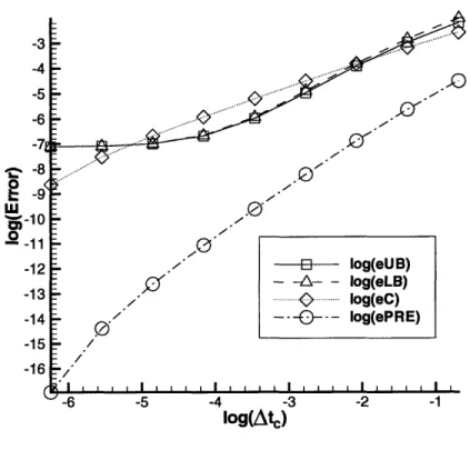
Figure 4-1: Convergence of Bounds with Respect to Coarse Mesh Element Size

is independent of n, one LU decomposition suffices. Fifth, and finally, the results of steps four and five are used to evaluate Equation 4.17 to find the bounds. Step five requires a number of matrix multiplications, but as each time step contributes independently, this step can also be easily parallelized. Steps three, four, and five must each be executed twice, once for the upper bound and once for the lower bound. Altering the size of the coarse mesh affects the time required for steps one and two of the calculation without affecting the later steps at all. Therefore, it might be most efficient to refine the coarse mesh to a point where the coarse mesh calculation requires perhaps one order of magnitude less time than the truth mesh calculation. The time required for the latter three steps is fixed by the resolution requirements of the truth mesh. If steps three, four, and five require one hour to compute, it might make sense to choose a coarse mesh requiring perhaps five minutes to solve. The difference between a five minute coarse mesh and a thirty second coarse mesh does not greatly impact the total solution time, but the added accuracy of the adjoint approximation can drastically reduce the gap between the bounds.

This approach is convergent as seen in Figure 4-1, where eUB is the upper bound error, eLB is the lower bound error, eC is the coarse mesh output error, ePRE is the error in the average of the upper and lower bounds, and Atc is the coarse mesh time step. The bounds grow closer together as the coarse mesh grows closer to the truth mesh. However, the use of the energy inequality instead of the energy equality introduces a small amount of error. As the coarse mesh approaches the

truth mesh, errors due to the quality of the adjoint approximation which dominate the total error for very coarse meshes become negligible compared to errors stemming from the inequality. This phenomenon limits the usefulness of the method because the accuracy needed in the bounds may prove impossible to achieve even with an extremely fine coarse mesh as illustrated by the flattening of the error graph for the bounds as Ate shrinks in Figure 4-1. The additional source of error results in the need for more work to achieve the same accuracy as would be present without the inequality.

This method is rather simple to implement but, because of the inequality, not so effective. It does, however, illustrate the general approach to bound formation as well as reveal some of the more serious difficulties inherent in solving time-dependent problems.

Chapter 5

Second Approach: Finite

Elements in Space, Spectral

Elements in Time

The second approach avoids the problems caused by the energy inequality in the first approach. The primary difference between the two approaches regards the way the temporal aspect of the problem is treated. In the first approach time was discretized using a backward Euler finite difference scheme. The second approach uses spectral elements in time [6]. Appendix B describes the basis functions, quadrature schemes, and other nuances of spectral elements. The use of spectral elements in time is usually a very poor choice for parabolic partial differential equations because of the enormous amount of temporal coupling it tends to introduce. In this particular case using spectral elements is an excellent choice because the unusual circumstances actually lead to total decoupling of the equations in time.

Once again the strong formulation of the problem is the starting point:

Ot(x, t) = aOOx(x, t) - /O(x, t), (5.1)

e(x, o) = 0 (x), (5.2)

Ox (0, t) = Ox (1, t) = 0. (5.3)

To arrive at the weak form necessary to state the finite element problem, the inner product of an arbitrary function, v, and the strong equation is integrated over the spatial domain. The initial condition is also weakly incorporated to arrive at the following form:

0

The inner product represents a form of time integration over the domain. For an arbitrary v E L2, satisfaction of this equation ensures agreement with the strong

form.

the solution to be weakened. Some of the relaxation of constraints is done through integration by parts to transfer derivatives from the field variable, 8, to the test function, v. Therefore, to be effective, the inner product must allow integration by parts to proceed in the same fashion as with standard time integration. To that end, the inner product must satisfy

(V, 9t) = v(x, 1)0(x, 1) - v(x, O)0(x, 0) - (vt, 0) (5.5)

and

o(, Oxx)dx = (v(1,t), Ox(1, t)) - (v(O, t), O(0, t)) -

fo

Using these properties to integrate Equation 5.4 by parts and substituting the ho-mogeneous Neumann boundary conditions of Equation 5.3 into the result yields the final weak form,

Sv(x, 1)(x, 1)dx - (vt, O)dx + a (v, Ox)dx + P (v, )dx

-1 _{v(x,O)o(x)dx = 0. (5.7)}

As in the first approach, to form the quadratic minimizable form, the energy equality, from the weak form, v is set equal to 0. Symmetry of the inner product and Equation 5.5 allow the second term in the energy equality to be simplified:

- (Ot, O)dx = -2(x, 1) + 2 (x, 0). (5.8)

The energy equality can be written as a general functional of an arbitrary function,

v, which vanishes when v = 8,

E(v) = v2(, )d + v2(x, O)dx + a (vX, vX)dx + (v, v)d

-fo v(x, 0)0o(x)dx. (5.9)

All of the terms in the energy equality, save the last one, are positive definite and quadratic. The last term is linear. Therefore, the energy equality is a quadratic minimizable functional which vanishes when v = 0, and it can serve as the functional

to minimize in the constrained minimization problem that will generate the bounds. The output functional, the average over space and time, can be written in terms of an inner product,

i(v) = (v, 1)dx, (5.10)

£(9) = s. (5.11)

Augmenting the energy equality with the linear output functional once again results in a quadratic minimizable form which reduces to ±s when v = 0. As before, the

augmented functional is defined

S+(v) = E(v) ±e (v), (5.12)

S(v) = v2(X 1) + v2 (x, O)dx + a (vX, vX)dx + 0 (v,

v)dx-fo

1

The weak form itself, Equation 5.7, can be written in the more general form of a Lagrange multiplier constraint enforcing v = 0,

1 (x, 1)v(x, 1)dx - j(it,v)dx + a (iix, v)dx + (p, v)dx

-f (x, O)Oo(x)dx = 0. (5.14)

For Equation 5.14 to be satisfied for an arbitrary /t, v must equal 0.

Because S+(O) = ±s, trivially

Is = minS (v). (5.15)

v=0

The constraint that v = 0 is equivalent to the constraint that Equation 5.14 be

satisfied for an arbitrary Lagrange multiplier functions, A. Therefore, a Lagrangian can be formed to transform the constrained minimization problem of Equation 5.15 into the min-max problem

S(,

) = v2 _{1)dx 1 2(, O)dx + a (v, vx)dx + f (v, v)dx}

-o v(x, O)O-o (x)dx f(v, 1)dx + fo p(x, 1)v(x, 1)dx

-j(pt, v)dx + a j(x, 7v)dx + ₁ (IL, v)dx

-fop(x, 0)Oo (x)dx, (5.16)

± s = min max± +(y, v). (5.17)

In other words, £~C(p, v) = is at the saddle point of the Lagrangian. At the saddle

point, v = 0 and / = +' , or £'(0f, 0) = ±s; 0± is known as the adjoint.

Satisfaction of the constraint in the Lagrangian produces the exact value of the output. Relaxation of the constraint produces bounds. To relax the constraint, first the minimization and maximization must be swapped as is permissible in the case of a saddle point,

i s = max min £+(p, v). (5.18)

The constraint is then relaxed by removing the maximization over the Lagrange The constraint is then relaxed by removing the maximization over the Lagrange

multiplier function. Since the Lagrangian was maximized by p = V', an arbitrary choice of p produces a value less than the maximum, is, a bound, i. e.

Ss > min±(p,, v) (5.19)

V

or

min £+ (p, v) < s < - min C-(p2, v). (5.20) The relaxation of the constraint effectively frees the approximate solution from sat-isfying the weak form exactly .

The primary calculation involved in finding bounds determines the v that mini-mizes the Lagrangian for a given p. This minimizing v is denoted 9±. The Lagrangian can be minimized with respect to v by setting to zero the first variation of the

La-grangian with respect to v:

6'C(t.0)=

j1

2a f(', + 2/6f (6±,6v)dx -,)dx 1 6v(x,0)9o(x)dx + l(Jv, 1)dx + j f(x, 1)6v(x, 1)dx -

j(i,

(j

(p , 6v)dx + ,

j

where F refers to the approximate guess for the adjoint.

The inner product and finite element spaces have thus far been left unspecified. The time discretization is set by the order of the Gauss-Legendre-Lobatto quadra-ture scheme used for the spectral elements. If the scheme uses N points, it exactly integrates polynomials of degree 2N - 3 or less. The inner product naturally implied by the quadrature scheme is

N

(v, w) E ,in v(tn)w(tn), (5.22)

n=1

where the tn are the quadrature points, and the n are the associated quadrature weights. The nature of the integration scheme points to a polynomial finite element space. The maximum degree of polynomial fully specifiable with one point value at each quadrature point is N - 1. The set of degree N - 1 polynomials, i (t), that satisfy &i(tn) = 6in forms a basis for the space. Additionally, these basis functions are

orthogonal in the given inner product. If Af, 0±, and 6v are restricted to be members of this space, they can be represented as weighted summations of the basis functions,

N ±(x, t) = 1 an(x)G(t) (5.23) n-1 N 0±(x, t) = E bn(x)n (t) (5.24) n-1

N

6v(x,t) = E d(x) n(t). (5.25)

n-1

The coefficients of these basis functions for A', 6v, and 0± vary in space within the prescribed definition of the spatial finite element space. If the finite element space is chosen to be the set of functions over the domain which are piecewise linear on Nx equally sized sections of space, the elements, whose boundaries are known as nodes, then the basis functions are the standard hat functions, qi(x), centered on each node, xi, _{where Oi(xj) =} 6ij. _{The spatially varying coefficients in Equations 5.23,} 5.24, and 5.25 can be written as weighted summations of the basis functions so that Equations 5.23, 5.24, and 5.25 can be rewritten

N N,+1 = E i(x)e(t), (5.26) 1=1 i=1 N N,+1 ± =

Z

Following a standard Galerkin procedure of setting 6v = Oj(x) n(t), and substi-tuting the finite element function definitions of Equations 5.26 and 5.27 into Equa-tion 5.21 yields the following relaEqua-tionship between the approximate 0 coefficients and the coefficients of the approximate adjoint:

[(6nl + 6nN + 2,L3fin)M + 2afi34- = 6nif T find - [(6nN +

A3i)M

fnMP+D., (5.29)

where M is the mass matrix of hat functions defined by Mij =

10

K is the stiffness matrix of hat functions defined by Kij =

j

6n is the vector of all coefficient values at quadrature point n and similarly for E , f

is the vector defined by

fi = i (x)(x) dx

d is the vector defined by

di = i(x)dx, O

Di is the vector of spectral basis function derivatives at quadrature point i such that

and p+ is the matrix of all the coefficients of [+.

Finding a good approximation for the adjoint is not as trivial as in the first approach. In the above calculation of the approximate field solution, 0+, from a given approximate adjoint, the benefit of orthogonality of the spectral element basis functions decouples the equations in time. Spectral basis functions are not orthogonal with their time derivatives. In Equation 5.21, the dense vector of derivatives, D,, acts on the known adjoint. An attempt to solve the original system on a coarse grid with the spectral elements in time would result in a fully coupled system across all time because the derivative matrix would operate on the unknown value of the field variable. The solution of the dense system would be a highly inefficient way to arrive at an approximate adjoint.

A far more efficient way to calculate an approximate adjoint is by discretizing Equation 5.21 with the linear finite element and backward Euler finite difference scheme of the first approach, choosing the inner product to be true time integration and applying the continuous adjoint boundary condition of Appendix A. The sub-script of c denotes quantities calculated on the coarse mesh. The coarse mesh field solution, Oc, is calculated as in the first approach. The boundary condition from Appendix A is

"Nt= Nt. _(5.30)

The backward evolution equation for the adjoint is then

((1 + 3At)M + aAtK)~ ~ = M ± + T~ _{Atd - (2aAtK + 2pAtM) n}

n=N-1,.-.,0. (5.31)

The bilinear interpolant of V)± on the truth mesh can be used as an approximate adjoint, fi.

With the values for the approximate field solution and adjoint, the bounds, r+ and 7-, can be constructed by substituting these values into the Lagrangian. The Lagrangian can be written as a function of the finite element and spectral element coefficients as follows: 1 ± T _± 1 -T + N -iT O M - T N- MON + -1 1 E ,n (oK + M)_ - f a d + 2 2n=1 n=1 N n=1

-4-0' -6 -1 ... 0 .... . Iog(eC) -18 - ---- log(ePRE) -9 -8 -7 -6 -5 -4 -3 -2 -1 log(Atc)

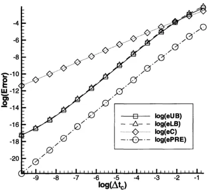
Figure 5-1: Convergence of Bounds with Respect to Coarse Mesh Element Size

coefficients in 0, 0. From Equation 5.20

77+ s _ -r-. (5.33)

Thus are the bounds formed.

The second method has some distinct computational advantages over the first method. Equation 5.29 illustrates one advantage of using spectral elements. Though spectral elements provide much better accuracy than backward Euler for the same number of temporal points, Equation 5.29 is decoupled in time in the same fashion as Equation 4.23 and requires the same amount of effort to solve. As before, the computational steps required to solve Equation 5.29 are eminently suitable for parallel computation. Second, the use of the energy equality instead of an energy inequality removes a significant source of error from the calculations. Also, since the same method is used in both approaches to calculate an approximate adjoint including the calculation of the coarse mesh solution, the spectral element method requires no more work than backward Euler to construct an approximate adjoint of similar quality.

Figure 5-1 illustrates the convergence of the method. In the figure, as Ate, the size of the coarse mesh time step, decreases, the resolution of the coarse mesh increases, and the errors drop; eUB is the error in the upper bound, eLB is the error in the lower bound, eC is the error in the output calculated by applying the output functional to the coarse mesh solution, and ePRE is the error in the predicted value of the output constructed by averaging the upper and lower bounds. With increasing coarse mesh

resolution, the error in the bounds drops as the upper and lower bound converge toward the true output. The graph also illustrates the utility of the method as a predictive tool. The coarse mesh error represents the error in the output calculated by traditional methods on the given coarse mesh. For a given required error threshold, the graph demonstrates that traditional methods demand a coarse mesh with orders of magnitude more resolution than that required by the constrained minimization approach. The method does not guarantee bounds that are more accurate than the coarse mesh output, but, as the graph indicates, such bounds are possible.

The combined savings of the added accuracy of spectral elements and the decou-pling in time generated by the spectral elements ensure the viability of the bounding techniques described here as a rapid alternative to exact output calculation.

Chapter 6

Domain Decomposition

The previous two chapters demonstrate the viability of constrained minimization approaches for output bounding. A real implementation of such techniques would include a spatial decoupling technique called domain decomposition. Because the primary goal of this thesis is to extend constrained minimization techniques to time-dependent problems, domain decomposition is a tangential element. However, as real world application of these techniques relies upon the use of domain decomposition for tractable computation of bounds, this chapter is devoted to a discussion of how domain decomposition is incorporated into constrained minimization techniques for temporal problems using spectral elements in time.

Domain decomposition divides a problem spatially into subdomains and, thus, partially decouples the solution process and produces a strong computational advan-tage. Much of the computational advantage does not come to bear until a second space dimension is added to the problem, but the simpler problem described here acts as proof of principle for the method. The use of spectral elements and the use of domain decomposition are independent; one can be used without the other. Here they are illustrated working in concert.

The standard constrained minimization technique uses a Lagrange multiplier func-tion to enforce the original finite element equafunc-tions. In order to utilize domain decom-position, a second constraint must be added to the system. If the problem domain is subdivided into M sections, the problem statement can be relaxed by allowing the field solution to have jump discontinuities across the subdomain boundaries. In order to retrieve the original continuous solution, a Lagrange multiplier function can be used to enforce continuity across the subdomain boundaries. This constraint takes the form

M-1

E ((m(t), V(Xm+11, t) - V(Xm2, t)) = 0, (6.1)

m=1l

where the Lagrange multiplier function, (, is continuous in time but only exists at the spatial interfaces between subdomains;

,m

at the right-hand boundary of subdomain m; and xm, and Xm2 are the limiting values

of x at the left and right ends of subdomain m, respectively. Equation 6.1 is only satisfied for an arbitrary ( if v is continuous across all subdomain boundaries.

Adding this constraint to the original Lagrangian of Equation 5.16 yields a new Lagrangian that allows 0 to have jump discontinuities across subdomain boundaries but then enforces continuity across the same subdomain boundaries by means of a Lagrange multiplier function,

Sv) v2(, 1)dx + 2(,)d (O), + Vx)dx +/

(v,v)dx-j

_fo

S

As before, at the saddle point of the Lagrangian, v = 0, the field solution and p - +,

the adjoint, and now C = w+, known as the hybrid flux. The bounds are formed by

relaxing the constraints and solving the minimization problem for arbritrary Lagrange multiplier functions,

min C+(pt, (1, v) < s < - min E-(p2, 2 , v). (6.4)

V V

The relaxation of constraints frees the approximate solution from satisfying the weak form exactly and allows it to have jump discontinuities across subdomain boundaries. For given approximate Lagrange multiplier functions,

f

(*, (+, 0+) = + (x, 1) 6v (x, 1)dx + (x, 0) 6v (x, 0) dx + 2a (O

,

The hybrid flux is a continuous function in space but only exists at discrete points in space, the subdomain boundaries. Like f and 0, ( can be written as a linear

combination of spectral basis functions: N

E(t)

= E nmn (t), m = 1, ..., M - 1. (6.6)

n-1

In order to enable the finite element space to contain spatially discontinuous func-tions, the nodes at subdomain boundaries need to be split into double nodes with the hat function centered on the left node truncated to the right of the node and the hat function centered on the right node truncated to the left of the node as is typically done with the hat functions on the edges of the domain. The approximate adjoint and the corresponding field solution, 0, can be written in terms of the discontinuous basis functions as N Nx+M E E

S

5

Substituting these representations of the functions into Equation 6.5 and following

the Galerkin procedure of setting 6v = ($(x) n(t) yields a relationship between the

coefficients of the approximate 0 and those of the corresponding approximate adjoint and hybrid flux,

[(6fnl + 6nN -+ 2/&)M + 2CenK]#n 6nlf T &ind - [(6nN -+ /3P,) M

+

-M±V - (6.9)

where C is the vector of all coefficient values of the approximate hybrid flux at quadrature point n, and V is the matrix defined by

Vij = i,j+1 - ij2

where i is the number of a node, j + 11 is the number of the node on the left side of subdomain j + _{1, and j2 is the number of the node on the right side of subdomain j.} The approximate adjoint is calculated as in the previous chapter; however, conti-nuity of the adjoint is enforced, so the hybrid flux contributions cancel out, thereby reducing Equation 6.9 to Equation 5.29. To calculate an approximate hybrid flux on the same coarse mesh, the discontinuous formulation must be retained. This is done by following the same procedure as for the approximate adjoint but choosing the test functions, Sv, to be ramp functions, oj(x), piecewise linear functions by subdomain which are zero at the left edge of subdomain j, one at the right edge of subdomain

j, and zero in the remaining subdomains. The matrices Q and R and the vector g are defined by