by
William K. Dewar
B.S. the Ohio State University (1977)
S.M. the Massachusetts Institute of Technology (1980)
SUBMITTED IN PARTIAL FULFILLMENT OF THE REQUIREMENTS FOR THE DEGREE OF
DOCTOR OF PHILOSOPHY
at the
MASSACHUSETTS INSTITUTE OF TECHNOLOGY and the
WOODS HOLE OCEANOGRAPHIC INSTITUTION October 1982
Signature of Author _ _ _ _ __ __
Department of Meteorology and Physical Oceanography, Massachusetts Institute of Technology and the Joint Program in Oceanography, Massachusetts Institute of Technology/Woods Hole Oceanographic Institution, October, 1982.
Certified by i Thesis Supervisor
Accepted by
Chairman, Jo t Committee for Physical ceanography, Massachusetts Institute of
Vechnology/Woods
Hole Oceaqographic Institution.FRO
C y
.IT
ATMOSPHERIC INTERACTIONS WITH GULF STREAM RINGS by
William K. Dewar
Submitted to the MIT-WHOI Joint Program in Physical Oceanography on 8 October, 1982
in partial fulfillment of the requirements for the degree of Doctor of Philosophy
ABSTRACT
Four different problems concerning Gulf Stream Rings are considered. The first deals with the particle trajectories of, and advection-diffusion by, a dynamic model of a Ring. It is found that the streaklines computed from the assumptions that the Ring is a steadily propagating and permanent form structure accurately describe its Lagrangian trajectories. The dispersion field of the Ring produces east-west asymmetries in the streaklines, not contained in earlier kinematic studies, which are consistent with observed surface patterns. In the second problem, we compute the core mixed layer evolution of both warm and cold Rings, and compare them to the background SST, in an effort to explain observed SST cycles of Rings. We demonstrate that warm Rings retain their anomalous surface identity, while cold Rings do not, because of differences in both the local atmospheric states of the Sargasso and the Slope and the typical mixed layer structures appropriate to each. The third and fourth problems concern the forced evolution of Gulf Stream Rings as effected by atmospheric interactions. First, we compute the forced spin down of a Gulf Stream Ring. The variations in surface stress across the Ring necessary to spin it down are caused by the variations in relative air-sea velocity, of which the stress is a quadratric function. From numerical simulations, we find the forced decay rates are comparable to those inferred from Ring observations. In the final problem, it is suggested that a substantial fraction of meridional Ring migration is a forced response, caused by Ring SST and the temperature dependence of stress. The warm central waters of anticyclonic Rings are regions of enhanced stress, producing upwelling to the north, and downwelling to the south, which shifts the Ring to the south. A similar, southward shift is computed for cyclonic Rings with cold centers, which tends to reconcile their numerically computed propagation with observations.
TABLE OF CONTENTS
Title Page ... 1
Abstract ... ... *...*... ... 2
Table of Contents ... ... 3
Chapter I. Introduction ... 7
Ring Observations and Description ... 8
Contents ... * * ... ... ***** * 10
Chapter II. Preliminaries ... 15
a. Introduction ... 15
b. The Quasi-Geostrophic Horizontal Structure Equation ... *...*... 15
The Equivalent Barotropic Equation ... 25
A Discussion of Baroclinic Instability ... 26
c. Advection-Diffusion of a Passive Scalar ... 27
d. The Mixed Layer ... 28
Conservation of Mass and Thermodynamic Energy ... 29
Momentum Equations ... 31
Quasi-Geostrophic Scaling ... 32
Ekman Pumping ... 34
Energy Equation ... 35
Wind Wave Breaking and Penetrative Convection ... 38
The Froude Number and Its Value ... 39
e. Numerical Techniques ... 40
Chapter III. Particle Trajectories in Numerical Gulf Stream Rings ... 41
a. Introduction ... 41
Ring Model ...*. ... .. 45
b. Kinematic Models ... 46
Tracer Diffusion in Kinematic Models ... 49
Tracer Homogenization on Closed Streamlines ... 49
c. Advection and Diffusion in a Dynamic Ring Model .. 62
Dynamic 'Streaklines' ... 64
The Importance of the Dispersion Field ... 70
Advection-Diffusion Using Dynamical Advection Fields ... 72
Ciritcal Contour ... 75
Exterior Streaklines ... 75
d. Potential Vorticity Considerations ... 80
Ring Exterior ... 83
e. Implications ... 84
Chapter IV. An Annual Mixed Layer Model with
Application to Gulf Stream Rings ... 90 a. Introduction ...
Background ... b. An Annual Mixed Layer Model ... c. Limit Cycle Calculations ... 'Typical' Mixed Layers ... d. Adjustment Calculations ... e. Summary ...
Appendix A.IV. A Bulk Mixed Layer Model ... 121 a. The Equations and the Forcing Functions ...
Meteorological and Solar Data ... Winds ... ...
Air Temperature ... Solar Heating ... b. Initial Experiments with the Thompson Model .. Appendix B.IV. The Sensitivity of Mixed Layer
Development to Buoyancy Flux ... ....131 The Reformation of the Thermocline ... 131 Wintertime Mixed Layers ... 135 Appendix C.IV. Verification of the Annual Mixed Layer
Equations ... Choice of h ... ... 139 Validation ... 140 90 90 95 101 103 109 117 121 123 123 124 124 127 ... 139 ~
Chapter V. The Wind Forced Spin Down of Gulf Stream
Rings ... 144
a. Introduction ... 144
Observations of Ring Decay ... 145
b. Ekman Pumping ... 150
c. Planetary Wave Spin Down ... 153
d. Nonlinear Vortex Spin Down ... 157
Barotropic Mode Scaling ... 157
Parameters ... 158
Unforced Results ... .... . ...*159
Forced Results ... ... 160
The Relative Importance of Forcing ... 167
e. Parameter Variations ... ....169
f. The Spin Down Mechanism ... 171
g. Summary ... .... 176
Appendix A.V. Chapter VI. Wind Stress in the Presence of Surface Flows ... 178
Southward Ring Propagation as a Consequence of Surface Temperature Anomalies ... 184
a. Introduction ... 184
b. Scale Estimates ... 187
The Coefficient of Drag ... 187
The Ekman Divergence ... 189
The Pumping and Its Effects ... 189
c. Governing Equations ... 192 d. Numerical Results ... 195 Parameter Studies ... 204 e. Discussion ... 205 Integral Constraints ... 206 Zonal Propagation ... 209 Meridional Propagation ... 210
f. Potential Vorticity Budgets ... 211
VII. Summary ... ... 220
Suggestions ... ... ..223
References ... 226
CHAPTER I. INTRODUCTION
Gulf Stream Rings are intense vortices shed by the Gulf Stream, characterized by velocities up to 150 cm/sec and diameters of about 100 km. They are commonly found in the Slope Water and the Sargasso, and as such constitute the most energetic time dependent phenomena in either region. Rings transport water between the Slope Water and the Sargasso, which has led scientists to suggest that they are a dominant component in the heat and energy budgets of both regions. For example, the potential vorticity flux to the Sargasso caused by Rings has been
estimated at 1 m2/sec2, which is the same magnitude as that due to the atmosphere (the Ring Group, 1981). Similar statements apply to Ring-induced salt and heat flux. In addition, the powerful velocities of a Ring can strain existing tracer gradients, enhancing their diffusive transport. Thus, it is very likely that Rings are important to the large scale picture of the oceans. Whether Rings produce effects as large as these estimates, or alter their environment in a significant way, is the focus of current observational and theoretical effort
(Richardson, 1980).
The areas essential to addressing these questions, in which our knowledge is incomplete, include Ring decay, propagation, and
transport. Recent modeling efforts (McWilliams and Flierl, 1979; Mied and Lindemann, 1979; Ikeda, 1981; Nof, 1980; Flierl, 1982) have centered on the evolution of freely evolving structures imbedded in a resting body of water. Although several of these studies have mentioned the
potential importance of mean state advection and external forcing, there have been only a few attempts at including shear (Flierl, 1979) and wind stress (Stern, 1965) in eddy calculations. In the present thesis, we will consider how atmospheric forcing affects the evolution of Rings,
and demonstrate that several of their oceanographically important properties are significantly influenced by air-sea exchange. In particular, we shall see that Ring decay and propagation are affected by wind forcing, and that the evolution of Ring surface waters is sensitive to diabatic heating. Also, because many of the processes involved in these problems are more naturally discussed in a Lagrangian frame, and because of the importance of Ring advection on their surroundings, we have computed the particle trajectories of a Gulf Stream Ring.
Ring Observations and
Description-Rings are distinguished from the mesoscale variability of the North Atlantic primarily in two ways. First, they undergo a unique formation process: Gulf Stream meanders grow to finite amplitude, close, and subsequently separate from the current. Second, Rings carry with them a sizeable volume of distinctive water. Ring production has been observed to occur on both sides of the stream, producing vortices of positive (cyclonic) rotation to the south and negative (anticyclonic) rotation to the north. Similar structures are found in the vicinity of most major current systems (Hamon, 1960; Nilsson, Andrews, and Scully-Power, 1977; Kawai, 1979), although presently, the literature is most complete for
The first well documented long term observation of a single Ring (cyclonic) is due to Fuglister (1977), who was able to track the same Ring for six months. To date, several Rings have been tracked (Richardson, 1980) and many of their common physical properties catalogued. Rings persist as recognizable coherent structures, literally as closed loops of flow, for years at a time (Parker, 1971). They translate toward the west-southwest at speeds of about 5 cm/sec but can exhibit rapid eastward motion when interacting with the Gulf Stream. As many as 10 cyclonic and 6 anti-cyclonic Rings have been
observed to coexist. They are formed at a rate of about 7 Rings per year and are frequently removed from the general circulation by
reabsorption into the Gulf Stream (Richardson, 1980). For a more complete descriptive review of Rings, see Lai and Richardson (1977).
During formation, large pieces of water are trapped within the closing meanders which results in Rings having a peculiar water mass composition. For example, a cyclonic Ring in the Sargasso Sea will have an interior consisting of Slope Water. The strong temperature contrasts between the Slope water and the Sargasso have led to the now standard labels of 'cold core Ring' for those found in the Sargasso, and 'warm core Ring' for those in the Slope. The formation process also suggests some other terms which will be used in the present manuscript. The region into which the newly formed Ring moves will be referred to as the 'host region', and the area from which the core waters originated will be called the 'parent region'. As an example, the Sargasso Sea is the host region of a cold core Ring and the Slope Water the parent region.
Contents-The following brief summaries of each chapter will serve as a guide to the new results in this thesis.
Chapter III
Flierl (1981) computed the particle trajectories of a steadily-propagating, axisymmetric pressure pattern with closed streamlines. By
applying this model to Rings, he was able to make many useful statements with regards to the structure of particle tracks, trapped zone size, and averaged Lagrangian velocities. This study was purely kinematic, and employed a velocity field which turned out to be dynamically inconsistent, although it did come from an analysis of Ring data (Olson, 1980). In Chapter III, we conduct a Lagrangian analysis of a dynamically evolving Ring, the equivalent barotropic Ring model originally proposed by McWilliams and Flierl (1979). Comparisons between the dynamical model streaklines and those of the kinematic study are made which point out where the earlier calculations adequately describe particle motion and where improvements are needed. The particle trajectories of the dynamic Ring are investigated in terms of potential vorticity, and the importance of the dispersion field is discussed. We conclude Chapter III with an example of Ring interaction with tracer boundaries, performed with a view towards modeling Ring-thermal front interactions.
Chapter IV
In satellite infra-red images, Rings generally show up as well-defined pools of anomalously warm or cold water. Thus, one of the first
cycles to be observed by the remote sensing program was that of the annual Ring sea surface temperature. It is now documented that cold core Ring surface waters do not survive beyond their first summer as an identifiable cold pool (the Ring Group, 1981); however, warm core Rings, with the possible exception of summertime, remain visible throughout their lifetime in satellite infra-red images. From XBT data, we find evidences of strong air-sea exchange and deep mixed layers in warm core Rings, and a curious lack of unusual surface water development in cold core Rings. In Chapter IV, we consider mixed layer evolution on the annual time scale, with particular emphasis on explaining the features of Ring SST cycles. Using a one dimensional model, we compare the forced response of the core surface layer of a Ring to that of its flank, demonstrating what aspects of the observed surface temperature field can be attributed to local air-sea exchange. This view differs from the pervading idea that it is the Ring dynamics which are responsible for the sea surface temperature (SST) behavior. We also apply the results of this study to the interpretation of satellite infra-red images. The model, within the restrictions of one-dimensionality, suggests how to objectively interpret SST anomalies.
Chapter V
Rings persist for years at a time (Lai and Richardson, 1977), although they do experience a recognizable aging process (Richardson, Maillard, and Sanford, 1981). Various estimates of decay rates have
been made using observed subsidence of isotherms (Parker, 1971) or loss of potential energy (Cheney and Richardson, 1976) and suggest lifetimes of roughly two-three years. One of the classic problems of Ring evolution concerns the method by which Rings lose their energy. It was concluded by McWilliams and Flierl (1979), as well as by Meid and Lindemann (1979), that vortex decay in their numerical experiments was strongly influenced by viscosity and that the usually dominant dispersive decay mechanism was in large prevented by the strength of the flow. The lack of a well-founded closure theory prevented them from making any definitive statements with regards to decay beyond a recognition of the importance of the weak non-conservative processes. In Chapter V, we investigate the possibility that Ring spin down is a result of Ekman divergence driven by local variations of momentum transfer at the sea surface. The bulk formula for stress is a quadratic function of the relative air-sea velocity; therefore, the presence of intense surface velocities can induce local, non-negligible, gradients of stress. The dissipative nature of the forcing, similar to bottom friction, emerges from the calculation of the Ekman pumping; one of the more useful results is the analytical expression for what corresponds to the coefficient of viscosity multiplying the frictional operator. A series of numerical experiments, including the pumping, are performed and the results compared to oceanic observations of Ring decay.
Chapter VI
In Chapter VI, we consider the effects of the local variations in stress on a Ring caused by its surface temperature field. The dependence of the bulk aerodynamic coefficient of drag on the temperature difference between the air and water has been documented by Deardorff (1968), and produces 0(50%) variations in stress for temperature contrasts on the order of a few degrees Centigrade. Ring surface temperature anomalies are such that both Ekman suction and pumping are produced, forcing the Ring to the south. We present numerical experiments, which include surface temperature anomalies, to demonstrate this effect and discuss the dynamical balances which account for the meridional propagation. McWilliams and Flierl (1979) point out that according to quasi-geostrophic dynamics, freely evolving cyclonic vortices (cold core Rings) move northward; a result which is counter to most observations. One of the interesting results of Chapter VI is that
both warm and cold core Rings are compelled towards southward motion, which brings the predicted propagation of cold Rings more into accord with observations.
Chapters II and VII
The relevant equations are derived and catalogued in Chapter II. First, we discuss a two degree of freedom quasigeostrophic model in both layered and continuously stratified modal forms (Flierl, 1978) and review the validity of the equivalent barotropic equation. This is followed by derivations of the advection-diffusion equation and the
basic mixed layer equations. Chapter VII contains a summary together with a discussion of future research topics suggested by this work.
Page
-15-CHAPTER II. PRELIMINARIES
II.a
Introduction-The purpose of this chapter is to derive and catalog the fundamental equations which we will frequently use. Necessarily, some of the content of the next few pages will not be new; for example, we review the derivation of the quasi-geostrophic modal equations as originally formulated by Flierl (1978). On the other hand, a rather original derivation of Ekman pumping as the upper boundary condition on the mesoscale will be presented in the section dealing with the mixed layer. In all sections, we will point out the relevant physics contained within each equation. The reader already familiar with general areas of quasi-geostrophy, advection-diffusion, and mixed layers can skip directly to Chapter III. It should be noted however that the notation employed in this chapter will become standard, thus reference to the tables and sections contained herein should resolve any questions with respect to symbol definition.
II.b The Quasi-Geostrophic Horizontal Structure
Equation-The basic equation describing the dynamics of the mesoscale is the quasi-geostrophic psuedo-potential vorticity conservation equation. In
dimensional form, this equation is:
2
y]
p + J- ( o )+foY = 0 Eq. II.1 - T--z 7 ' - z " f °0 ] = 0
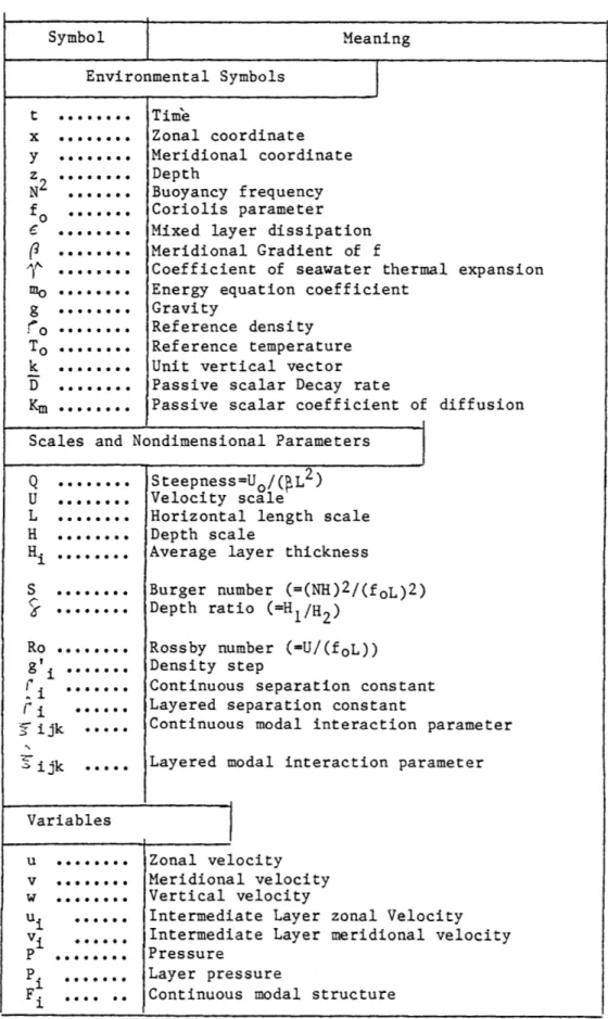
Table II.1 Symbols and Definitions Symbol Meaning Environmental Symbols t ... Time x ... Zonal coordinate y ... Meridional coordinate z ... Depth N2 . .. . . Buoyancy frequency fo ... Coriolis parameter
... Mixed layer dissipation ... Meridional Gradient of f
. ... Coefficient of seawater thermal expansion
mo . .. . . . .. . . Energy equation coefficient
g ... Gravity
o ******* Reference density
To ... Reference temperature k ... Unit vertical vector D ... Passive scalar Decay rate
Km ... Passive scalar coefficient of diffusion Scales and Nondimensional Parameters
Q ... Steepness=Uo/( L2)
U ... Velocity scale
L ... Horizontal length scale H ... Depth scale
Hi ... Average layer thickness
S ... Burger number (=(NH) 2/(foL)2) ... Depth ratio (=H
1/H2) Ro ... Rossby number (=U/(foL))
' ... Density step
fi ... Continuous separation constant
fi
... Layered separation constantSijk see** Continuous modal interaction parameter ijk ... Layered modal interaction parameter
Variables
u ... Zonal velocity v ... Meridional velocity w ... Vertical velocity
ui ... Intermediate Layer zonal Velocity vi 0*e Intermediate Layer meridional velocity P ... Pressure
P. ... Layer pressure
F .... .. Continuous modal structure
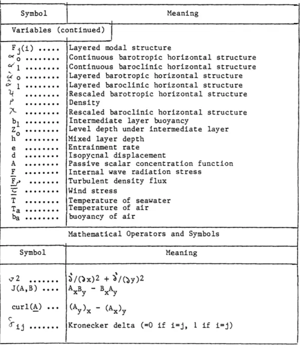
Table II.1 Symbols and Definitions (continued)
Symbol Meaning
Variables (continued)
Fj(i) ... Layered modal structure
o ***... Continuous barotropic horizontal structure ... Continuous baroclinic horizontal structure o ... * Layered barotropic horizontal structure
1 ... Layered baroclinic horizontal structure ... Rescaled barotropic horizontal structure
S... Density
.- ... Rescaled baroclinic horizontal structure
b1 . Intermediate layer buoyancy
Z ... *... Level depth under intermediate layer h ... Mixed layer depth
e ... Entrainment rate
d ... Isopycnal displacement
A ... Passive scalar concentration function F ... Internal wave radiation stress
F. ... Turbulent density flux
. ... Wind stress
T ... Temperature of seawater Ta ... Temperature of air ba ... buoyancy of air
Mathematical Operators and Symbols
Symbol Meaning
72 ... '/()x) 2 + 3/(4y)2 J(A,B) .... AxB - Bx y
curl(A) ... (Ay)x - (Ax)y
where d/dt, the substantial time derivative, is defined by:
d a 1 9 1
dt + J(P ) -- + (4 P ~ --- ). Eq. II.2
f dt f d " X y y x
o o
Eqs. II.1 and 2 describe exchanges between relative vorticity, vortex stretching, and planetary vorticity, along the horizontal projection of a particle trajectory, such that those exchanges conserve potential vorticity. For a complete derivation of this equation, see Pedlosky (1979). The proper vertical boundary conditions for Eq. II.1 are on the vertical velocity of the flow:
d/dt(Pz) = -N2w
at z=0 and -H. We will generally assume a flat bottom (w=0 at z=-H), but allow for a surface divergence. For horizontal boundary conditions, we shall assume for numerical purposes a doubly periodic domain:
P(x+Lx,y+Ly) = P(x,y).
Non-dimensionalizing x and y by L, t by (PL)-1, u and v by U, P by foUL, w by U2H/(foL2), and z by H (see Table II.1) returns:
[-+ QJ(P,.)][ p + P ] + 0, Eq. 11.3
St Jz S Jz + P=0x
where Q = U/(3L2), and S is the Burger number, defined by S = (NH)2/(foL)2. The vertical boundary conditions become:
C )
[--
+ QJ(P,.) ] -- P = -Sw Eq. 11.4:Jt %z
If the upper and lower boundary conditions are homogeneous, the linear form of Eq. II.1 becomes mathematically separable, and the vertical structure equation takes the Sturm-Liouville form:
1 2
j ( - F ) + F. = 0 Eq. 11.5
z S 2/z i 1 1
with:
(Fi)z - 0 at z = 0, -1,
where the separation constant, i is the non-dimensional Rossby Deformation Radius corresponding to the ith mode. We normalize the Fi according to: c
FiFjdz = 6ij.
-I
From Sturm-Liouville theory, we know the set of functions [Fil is complete, and therefore, we can write the pressure P as:
P(x,y,z,t) = i(x,y,t)Fi(z) Eq. 11.6 where
i = PFidz.
In general we cannot differentiate with respect to z under the summation sign in Eq. 11.6, for in the case of non-homogeneous top and bottom boundary conditions, the series will be non-uniformly convergent over the interval (-1,0). To obtain equations for the horizontal structure functions "ci, we employ a Galerkin approach (Finlayson, 1972), i.e. we operate on Eq. 11.3 with: I)
The resulting equation for the ith modal amplitude is:
(42 -[ 2)(&i)t + 7ijkQJ( ,(2-;k2) _ k) + (ii)x =
= Fi(O)Qwe Eq. 11.7
where:
0
- ijk = FiFjFkdz
is a coefficient representing the non-linear production of mode i from interactions of modes j and k. In later discussions, the evolution equations of Eqs. 11.7 will be referred to as the continuous equations.
It is useful to examine the results of a similar procedure on the quasi-geostrophic equations appropriate to a layered model. The nondimensional equation for the pressure in the ith layer may be written as: 2 2 f L [ + QJ( (P7 ) ] [P ( -P ) + it i giHi-1 i Eq. 11.8 2 2 fo0 (P - P
)
+-- P. = (forcing). I i+liwhere Q = U/(pL2) as before, Hi is the average thickness of layer i, and ' =
C(i
- i-i)/ o (see Fig. II.1). As in the continuous equations, we attempt a separable solution to the linearized form of Eq. 11.8:V
resting
P
depth
interfoce
Figure II.1. Schematic Diagram of a Two Layer Ocean
The dashed line represents the configuration of the interface for the resting state and 'd(x,y,t)' describes displacements of the interface related to geostrophic motion. Also shown are the average layer thicknesses, H1 and H2, and the layer densities -1 and C2- For a continuously stratified ocean, the density is described by the buoyancy frequency N2(z), and 'd' designates the fluctuations of isopycnals away from the mean state.
where <i represents a horizontal structure function, and Fj(i) the jth
eigenmode in the ith layer, which returns a separability condition in the form of a homogeneous tridiagonal matrix equation for the vector Fj(i):
22 2 2 f2
f L f f f
0 F .(i+1) )- + ] F .(i) + 0 F .(i-1) +
SH. H i i-1HgiHi
+ F .(i) = 0. Eq. 11.9
A'1
We normalize the [Fj(i)] by:
Fj(i)Fk(i)Hi = jk. Eq. II.10
The horizontal structure equations, governing the i, are: (72 -Fk 2Y)k + T ijkJ(ki,(72 - i'j2)cj) + (i)x =
- Fk(1)Qwe; Eq. II.11
we shall refer to Eqs. II. 11 as the layered equations. In form, Eqs. II.11 are identical to Eqs. 11.7, however there are important, subtle differences between the two involving the modal parameters, >ijk, k,
and Fk(1) for the layered case, and ijk, k, and Fk(0) for the continuous equations (see Table 11.2). Consider the baroclinic mode of a two layer model; all the baroclinic parameters, 5 111, 1, and F1(1),
Table 11.3 Layer and Continuous Modal Parameters
After Flierl (1978)
Continuous Two Layer
Barotropic F (z) .... ... 0 ... 1 .1 ist Baroclinic 1(0) ... 2.98 ... (H2/H1)1/2 4.66 x 10⁻⁴km- 2 ... H1(H2/HI)3/2 x 1/(H) .0000.0. 46.3 km ... -H2(H1)3 /2 x 1/((H2)3 /2H) (g'H1H2)1/2 x 1/(fo2H)) 1/2 111 ... 1.78 Rd1 .0 ... 0 0.... . ..
are specified by a choice of one density step, g'1, and one layer depth, Hl, assuming a value for the total depth H. That is, only two of the
three parameters are independent. In the analogous two modal case,
111, Fi, and Fi(0) are independent, reflecting a greater information
content in the continuous equations. Flierl (1978) has shown that the continuous equations are automatically 'calibrated' because all of the information about the mean stratification (in N2) is used to compute the modal structures, and hence the system parameters. In the presence of
surface forcing, Eqs. 11.7 are more accurate than the layered equations, and will be used in Chapters V and VI which are concerned with forced motion.
Note that if we = 0, the number of continous modal parameters in Eq. II. 7 is reduced to two ('ijk and k), the same number as in the unforced layered equations. In this case, the layered system is isomorphic to the continuous system and we are free to interpret the calculations in either frame. Generally, the two layered system is more intuitive, so it is this system in which we will interpret the advection diffusion calculations of Chapter III. The conversions between modal amplitudes and layer pressures for the two layer unforced case are given by:
c +S/21 = PI,
and: Eq. II.12
'o -1/ri = P2, where = Hi/H2 .
In Chapter V, we will need to calculate d, the deviation of an isopycnal from its resting depth (see Fig. II.1). The formula we will use is:
d = -Pz/N2 = -(T<(Fi))/N2, Eq. 11.13
which may be obtained by operating on the hydrostatic equation with: [ .f 2(Fz)/N2]dz,
and using the quasi-geostrophic equation: -N2d = b.
The Equivalent Barotropic
Equation-We obtain a two degree-of-freedom model if we retain only the two lowest modes in Eqs. 11.7. Such a model has been used to study a variety of oceanic problems (Flierl, 1978). Under certain circumstances, we may simplify the equations further to a single formula known as the equivalent barotropic equation.
(q2 - 12)Xt + QIIIJ( ,(7 2 - p2)c) +Cx = Eq. 11.14 = forcing - dissipation.
In this subsection, we will discuss the unforced (we=O) layered equations (recall the isomorphism) to illustrate the physical system
that Eq. 11.14 describes.
From Eq. 11.12, we see that the condition for a resting lower layer, P2 = 0, is:
10o = 1C1 . Eq. 11.15
However, if P2=0, Eq. 11.8 with i=2 becomes: (P1)t = 0.
Obviously, it is essential for the existence of time dependent flow that the lower layer not be strictly at rest. A proper interpretation of Eq. 11.15 is that for weak lower layer flows, the ratio co/"1 is 0( 1/2), as occurred in the numerical experiments of McWilliams and Flierl (1979), where the lower layer developed as an incoherent 0(51/ 2) wave field. If P1 = 0(1), we see 0C1 = 0( /2), and
therefore, "o = 0(6). Introducing the rescaled modal amplitudes:
and
<1 ~ 1/2,
into the layer equations, the lowest order in ~1/2 (<<1) is:
(V2 - -2)t + Qj(-,(- 2 - -2)) + x = 0, and a. Eq. 11.16 (q2-) t + QJ(X, (2 - r2)X) + ' x = 0. b.
We shall be primarily concerned with Eq. II.16.a, the equivalent barotropic equation, which we see, if we = 0, is the governing equation for the first baroclinic mode of a two layer fluid with a thin upper layer. Extensions of the present scaling arguments to the case we A 0 will be made later.
A Discussion of Baroclinic
Instability-The lack of mode-mode transfers excludes baroclinic instability from Eq. 11.14. This may be seen by multiplying Eq. 11.7, with i=1, by
<I and area averaging, assuming either no flow at eo or periodic boundary conditions. We obtain:
S(((~1)2 + 1-2 a 2 )/2)dA]t jc 1 ,( 2 - 'i2)'~l)dA, Eq. II.17
JJ
energy conversion between the barotropic and baroclinic modes, or baroclinic instability processes. By previous scaling, the right hand side is O( ) compared to the left hand side, and therefore negligible. While for some applications the lack of baroclinic instability might represent a shortcoming, the problems under consideration in the present thesis are not likely to be strongly affected.
II.c Advection-Diffusion of a Passive
Scalar-If a fluid parcel is convecting a passive tracer, A, the evolution of A is governed by:
At + u.VA = D + KmV2A Eq. II.18
where D symbolizes decay and Km molecular diffusivity. If we average (< >) Eq. 11.18 in some suitable way, we obtain:
<A>t + <u>. <A> = -V.<u'A'> + <D> + K 2<A>,
with coherent small scale transport providing a source for the mean fields. We will employ Fickian diffusion as a turbulent closure:
Fi = <u'iA'> = -KijAxj; Eq. 11.19 therefore, the equation for A becomes:
<A>t +<uj><A>xj = <D> + (Kij<A>xj)xi, Eq. 11.20 where we have neglected molecular processes.
From field measurements and laboratory work, it is known that turbulent mixing in the ocean is highly anisotropic, due to stratification, and that tracer transport occurs principally along density surfaces. The diffusivity tensor we will use, the only non-zero elements of which are on the main diagonal, models this anisotropy by
assigning a value to the vertical mixing coefficient which is orders of magnitude smaller than those of the horizontal coefficients. Hence, on the mesoscale, A is governed by (dropping brackets):
At + u.i7A = K(Axx + Ayy) + D, Eq. 11.21
where we have ignored vertical (across isopycnal) mixing relative to horizontal (along isopycnal) and assumed Kij to be horizontally isotropic. We shall use only stable tracers, so D will be set to zero.
II.d The Mixed
Layer-The atmosphere forces the ocean via a layer in which small scale turbulent processes are important, and computation of their effect has become an area of much effort. One method consists of explicit computation of the turbulent fluctuations. These so-called deterministic models have proved to be very enlightening, although the required computational effort is large. A second approach is based on the observation that the upper layer is 'well mixed', which allows vertical derivatives to be neglected. Bulk models, as the latter are called, have proved to be reasonably accurate in their prediction of sea surface temperature, and appear to be simple enough to be included in large scale ocean models (Adamec, Elsberry, Garwood, and Haney, 1981).
In this thesis, we shall use a bulk mixed layer model and so will briefly outline the derivation of the bulk equations. Other discussions of the mixed layer can be found in Stevenson (1980) and Muller (1981).
Conservation of Mass and Thermodynamic
Energy-We model the ocean as a Boussinesq fluid:
4.u = 0, Eq. 11.22
Tt + uTx + vTy + wTz = KT,72T + Qz Eq. 11.23
where u represents velocity, T temperature, KT the coefficient of
thermal diffusivity, and Qz internal heat sources. Averaging Eq. 11.23 and using Eq. 11.22 returns:
Tt + uTx + vTy + wTz = KTq2T+ Qz - (w'T')z. Eq. 11.24
Here we have made the standard assumption that turbulent transfers are greater vertically than horizontally, or that (u'q')x, (v'q')y << (w'q')z where q is an arbitrary variable. A similar scaling will occur in all mixed layer equations.
We take the equation of state for seawater to be:
f= o(1-!(T-To)), Eq. 11.25
where 1o is a reference density, To a reference temperature, Y the coefficient of thermal expansion for seawater, and we have ignored salinity. Eq. 11.25 allows us to convert Eq. 11.24 to an equation governing buoyancy:
b =
-s-fo)/lo-bt + ubx + vby + wbz = -(w'b')z + K,2b + Boz, Eq. 11.26
where (Bo)z represents internal buoyancy sources. We suppose that the turbulent fluxes well-mix the upper layer, so that due to the lack of z dependence in the mean state variables, the vertical integration of Eq. 11.26 over the mixed layer depth, h, is trivial:
where we have neglected free surface variations and diffusion, and dropped the overbars on u,v, and b.
To close this equation in terms of mean variables, boundary conditions on the turbulent buoyancy flux need to be specified. The mechanisms of heat removal from the ocean surface include latent heat loss, sensible heat loss, and black body radiation, all of which may be evaluated using bulk empirical formulae and encapsulated in the form:
w'b']o = V'go(T-Ta) + c Eq. 11.28
where P is an empirical coefficient, Ta the atmospheric temperature, and c a bias of the heat flux deriving from the fact that evaporation can only cool the sea surface. From a least squares regression of air-sea temperature difference and measured surface heat flux, Frankignoul found a value of p=10-3 cm/sec (personal communication). Also, from analysis of bulk meteorological formulae for surface heat fluxes (such as in Thompson, 1974),
P
is found to be 1.5 x 10⁻³ cm/sec. The calculations performed in this thesis all used 3= 10-3 cm/sec. At z=-h, the mixed layer, if it is deepening, entrains cold water:w'b']-h = (bi-b)e, Eq. 11.29 where bi is the buoyancy beneath the mixed layer and:
e = ht+uhx+vhy+w]-h
If the mixed layer is not deepening, there is no heat flux at the interface, so:
w'b']-h = 0. Eq. 11.30.
Using Eqs. 11.28 and 29 in 27 returns:
where ba is the buoyancy appropriate to the temperature of the air: ba = tg (Ta- To)"
Finally, an accurate mixed layer model requires the computation of the density field in the so-called intermediate layer, i.e. the layer extending to a depth of deepest wintertime mixed layer penetration, but which feels direct atmospheric contact for only a fraction of the year. The intermediate layer buoyancy is governed by:
C) I J
Sb + u b. + v b. + w- b = -- (w'b') + B
-t i + x i Oy 1 z 1 zz o
Eq. II.32
Turbulent transport in the intermediate layer is generally weak compared to those in the mixed layer and to other heat transport processes in the intermediate layer (Stevenson, 1980); we shall neglect them. A more interesting comparison is to be made between the strength of the vertical convection of heat, w(bi)z, and radiative heating, (Bo)z. Evaluating a typical formula for penetrative radiation (Thompson, 1974) at a depth of 50 m, estimating bz by the N2 value 10- 6 sec-2, and w by 10-4 cm/sec (see Chapter V), we see:
wbz/(Bo)z = (10-4cm/sec)(10-6sec- 2)/( 3.3 x 10⁻⁸cm/sec3) = = 3 x 10⁻³ << 1,
indicating that at lowest order, we can neglect vertical heat convection in the intermediate layer.
Momentum
Equations-The averaged momentum equations are (dropping overbars where convenient and neglecting viscosity):
The upper boundary condition on the vertical momentum flux is given by the wind stress:
-w'u' ~I 0, Eq. 11.34
while the stress at the base of the mixed layer consists of both the entrainment of intermediate layer momentum, and the radiation of
internal waves:
-w'' h = (u-ul)e + F. Eq. 11.35
In most mixed layer models, the momentum flux by internal wave radiation is neglected (Niiler and Kraus, 1975) although it is potentially important in determining the amount of energy available for mixing (Kantha, 1975). Bell (1979) estimates that, because of F, inertial oscillations are damped out in roughly a week; however, it appears that for low frequencies,
o-
<< fo, momentum loss to F is unimportant(Pollard, 1970). Therefore, we take F = 0. The vertically integrated horizontal momentum equations are:
h(ut + uux + vuy + wuz - fv) = -hPx + Z-, (ul-u)e,
and Eq. 11.36
h(vt + uvx + vvy + wvz + fu) = -hPy + >+ (vl-v)e, and the vertical momentum equation is the hydrostatic balance:
Pz = b.
Quasi-Geostrophic
Scaling-For large-scale, low-frequency flows, the inertial momentum terms in Eq. 11.33 are O(Rossby number, hereafter Ro) with respect to the Coriolis acceleration, and can therefore at lowest order be neglected. Similarly, a scale estimate of the turbulent momentum transport based on
the wind stress, when compared to the Coriolis acceleration, is small, leaving a lowest order geostrophic balance in the upper layer:
fov = Px, fou = -Py*
A vertical integration of the hydrostatic balance relates the pressures at any two depths.
P(z) = P(Zo) +jbdz. Eq. 11.37
We shall choose Zo to correspond to a depth just below the deepest mixed layer penetration, and therefore a depth governed by quasi-geostrophic dynamics. Roughly speaking, Zo = 0(200 m). 'z' will correspond to a depth within the mixed layer. Substituting for P in the zonal geostrophic balance returns:
u = -PY/fo = -P(Zo)y/fo - ( bdz)y/fo = Eq. 11.38
= u(Zo) - (,bdz)y/fo.
The ratio of the two terms on the right hand side of Eq. 11.38 is: (Ab)Zo/(foUL) = (ab)Zo/(fo2L2Ro), Eq. 11.39
which will be small if Ab<< Rofo2L2/Zo. A typical Rossby number for a swift, large-scale flow is:
Ro - 0(30 cm sec-l/(l0-4 sec-i 6x106 cm)) = .05; therefore, for the ratio in Eq. 11.39 to be small:
Db << ((.05) 36x1012)/(108 10-4) = 1.8.
Note that for a Ring, u=0(100 cm/sec), and the allowable Lb is even larger. In any case, restricting our attention to sea surface buoyancy differences less than 1.8 cm/sec2 6,T < 9 OC), the lowest order, mixed layer, geostrophic balance reduces to:
The surface can support thermal gradients which, because of the thinness of the upper layer, are incapable of seriously perturbing the shallow pressure field.
Ekman
Pumping-The potential vorticity equation obtained from Eq. 11.33, which is valid in the mixed layer, is:
t + ux + v' - fowz + 3v = (Ly)xz - (Cx)yz Eq. II.41 where = vx - uy, and ( = w'u'. From Eq. 11.40, we can substitute
-(Zo) for the upper layer vorticity and v(Zo) for the upper layer meridional velocity. At Zo, the vorticity balance is that of quasi-geostrophic dynamics;
It + ux + v y + Pv]Zo = fowz(Zo), which allows us to rewrite Eq. 11.41 as:
-fowz+fowz(Zo) = curl(-)z. Eq. 11.42 Integrating from Z=O to the level surface z=Zo returns:
-fo(w(O)-w(Zo)) + fowz(Zo)Zo = curl(C(0)) - curl(T(Zo)). Eq. 11.43
1 2 3 4 5
At depth, turbulent stresses are weak, and we are ignoring internal wave radiation, hence we can neglect term 5. Applying the boundary condition w(O)=O leaves us with terms 2 and 3 on the left hand side of Eq. 11.43. Term 3 represents a correction to the vertical velocity at depth Zo due to the quasi-geostrophic divergences in the fluid above it; however, comparing terms 2 and 3 shows:
and we obtain the classical Ekman pumping upper boundary condition on the interior flow:
w(Zo) = w(0) + O(Zo/H) = k.curl(J(0))/(fo). Eq. 11.44
Energy
Equation-As the mixed layer equations now stand, we have 5 equations (2 momentum, hydrostatic balance, thermodynamic energy, and mass conservation) in six unknowns (u,v,p,b,e,h). The classical technique for closing this system of equations uses the overall energy budget of the mixed layer, careful derivations of which have been presented in Niiler and Krauss (1977) and Stevenson (1980). Here, we shall simply write down the energy equation, and discuss the relative importance of its several components.
Neglecting local storage of turbulent kinetic energy, the bulk energy equation is:
0
e((b - b.)h - (u - u ) = 2m 3/2+ B h- dz, Eq. 11.45
1 - i o o -h
a b c d e
where ui is the momentum of the intermediate layer, Bo the surface heat flux, and the dissipation. Term 'a' represents a measure of the energy needed to entrain and mix cold, heavy fluid over the layer's full vertical extent. Term 'b' is the amount of energy available in the shear at the naviface. Term 'c' represents direct turbulence generation at the surface by the wind, generally thought of as breaking waves, and
term 'd' the flux of potential energy through the surface due to heating and cooling. Finally, the last term represents the dissipation of
turbulent energy within the mixed layer, a term whose importance in turbulent erosion models has been pointed out by Stevenson (1979).
The sum of terms a and b represents the energetic stability of the mixed layer. Consider a simple gravitationally stable two layer system, with the upper layer characterized by velocity u and density b, and the lower layer by ui and bi . The bulk potential energy of the
1
system, to a depth of h+#h, is given by:
u o
-_ -b PEi =- zbdz = -bizdz +
z =-h-- 0
z=-h- h - ui - bzdz = (b-bi)h2/2 - bi(h+ h)2/2,
S-bii
and the total kinetic energy by: KEi = u2h/2 + ui2(h)/2.
Now suppose that the system mixes itself (?!) to a depth h+fh, and that the new layer is characterized by buoyancy b' and velocity u'. b' and u' can be computed from the conservation of heat and momentum:
b' = (bh+biC(h))/(h+ lh), and:
u' = (hu+('h)ui)/(h+ h). The new bulk potential energy is given by:
PEf= - b'zdz = b'(h+Eh)2/2 =
and the new kinetic energy by:
KEf= (h=h)u'2/2 =(hu+ hui)2/(2(h+4 h)).
Note that the change in potential energy: PEf - PEi = (b - bi )hh/2 + 0 h)2,
is positive; the potential energy has increased because cold fluid has mixed up and warm fluid down. The change in kinetic energy is negative:
KEf - KEi = -(u-ui)_h/2 + O( h)2,
in agreement with decreasing the shear in the flow. The change in the total energy of the layer is given by:
SEt = (KEf+PEf)-(KEi+PEi) = ((b-bl)h-(u-ui)2)6h/2.
Clearly, if Et is negative, more kinetic energy has been released than potential energy gained. Hence, in a system where:
(b-b i )h - (u-ui)2
is negative, a perturbation can draw energy from the shear, grow, and 'mix'. This is the basic dynamic erosion mechanism originally proposed by Pollard, Rhines, and Thompson (1973), in which the shear at the base of the mixed layer is due to the presence of wind driven inertial oscillations.
The time rate of change of total energy is:
d/dt(E) = E/St = ((b-bi)h-(u-ui)2),h/(2St) =
((b-bi)h-(u-ui) 2)e/2, Eq. 11.46
which is a one-dimensional version of the right hand side of Eq. 11.45. The only effect on Eq. 11.46 of two dimensionality would be the inclusion of a (v-vi)2 term. Thus, if Eq. 11.46 is negative, we expect mixing to occur, and drive the system back to a state of dynamic stability. If it is positive, i.e. if there is insufficient kinetic energy in the shear to generate a mixing event, mixing will occur only
if energy is transported into the region of the mixed layer base. The terms on the right hand side of Eq. 11.45 describe this transport and identify the sources as wind wave breaking and thermal convection, both of which we will neglect. There currently is a difference in opinion amongst mixed layer modelers as to whether it is appropriate to ignore
these effects, so we now marshal our relevant arguments.
Wind Wave Breaking and Penetrative
Convection-Recently, direct observations of upper layer turbulent dissipation have been made and numerical experiments which resolve turbulence have been performed, and some insight into the balance of the dissipation and energy generating mechanisms has been gained. For example, Klein and Coantic (1981) found that the surface wave turbulent field was largely dissipated in the upper few meters, and for mixed layers deeper than about 10 m, inclusion of wave breaking made no noticeable difference in
the evolution of the system. Similarly, Gargett, Sanford, and Osborn (1980) noted an increased dissipation in the upper 10 m of the ocean, which they interpreted as a loss of wave driven energy. Thompson (1981) demonstrated that the energy in the upper layer caused by a random field of whitecaps is strongly surface trapped, and conjectured that the most important property of breaking waves might well lie in their ability to mix wind momentum downwards. Hence, we shall equate term 'c' of Eq. 11.45 to a fraction of the total energy dissipation.
As to penetrative convection, Gargett, Sanford, and Osborn observed that the energy of descending cold water plumes is dissipated prior to
reaching the mixed layer base, and thus does not assist in deepening. The experiments of Klein and Coantic also exhibit a tendency for buoyant energy production to be balanced by dissipation, although under weak winds and strong cooling, an additional few meter deepening in a thirty meter layer was noted. Similar small increases in numerical mixed layer depths, due to penetrative convection, have been noticed by Mellor and Durbin (1975). Finally, comparisons of model predicted and observed sea surface temperature are generally better when using models without penetrative convection (Gill and Turner, 1976). Therefore, we shall assume that the surface potential energy flux is balanced by
dissipation.
The Froude Number Closure and Its
Value-The remaining terms in the energy equation are:
o
e((b-bi)h-(u-ui)2) = d Eq. 11.47
-k
where '' is the dissipation left after the above balances have been removed. For C' = 0, Eq. 11.47 reduces to either the Pollard, Rhines, and Thompson mixing closure:
F = ((u-ui)2 + (v-vi)2)/((b-bi)h) = 1, a. Eq. 11.48 or:
e = 0, b.
and is the energetic closure used in this thesis. We implement Eq. 11.48 by using 'b' if F < 1, and 'a' otherwise. Note, Price, Mooers, and Van Leer (1978) suggest that F = .6. We have opted to use F = 1 on the basis of Thompson (1976), who tested a mixed layer model based on
Eqs. 11.48 against various other models and found it returned the highest coherence between predicted and observed SST.
II.e Numerical
Techniques-We, have employed double Fourier expansions and spectral methods (Gottlieb and Orszag, 1977) when necessary to perform numerical solutions to the quasi-geostrophic equations. Time stepping was carried out using a leap frog scheme with implicit formulation of the viscous terms; the computational mode was suppressed by substituting a modified Euler time step at every 50th iteration (Roache, 1977). The remaining numerical calculations are referenced within the text. Finally, a fraction of the numerical calculations reported in this thesis are essentially repeats of some earlier numerical studies conducted by McWilliams and Flierl, the only difference being that they employed a finite difference technique. In Chapters III, V, and VI, we have referred to these calculations as McWilliams and Flierl's calculations, although, technically speaking, they have been performed by the author.
CHAPTER III. PARTICLE TRAJECTORIES IN NUMERICAL GULF STREAM RINGS
III.a
Introduction-There is abundant chemical, biological, and physical evidence that Gulf Stream Rings produce a sizeable net Lagrangian transport (the Ring Group, 1981), in which an individual Ring carries a volume of water.
Given the contrast in most oceanographically interesting quantities across the Northern Atlantic Gulf Stream, Ring transport is a potentially important component in the maintenance of North Atlantic tracer distributions.
Outside of the Ring 'trapped' fluid, we have evidence from satellite photographs of the sea surface temperature fields that particles undergo sizeable excursions. Warm core Rings apparently pull filaments of warm and cold water into the Slope Water during their interactions with the Gulf Stream or the Shelf-Slope Water front. A fraction of these filaments, or 'streamers', are observed to extend fully across the Slope water, and directly connect the Gulf Stream to the Shelf. The implications with respect to the heat and chemical budgets of the Slope are obvious, although to date no quantitative streamer-flux estimates have appeared in the literature. Cold Rings are observed to interact with the surface temperature expression of the Gulf Stream in a similar manner, pulling filaments of warm water into the Sargasso.
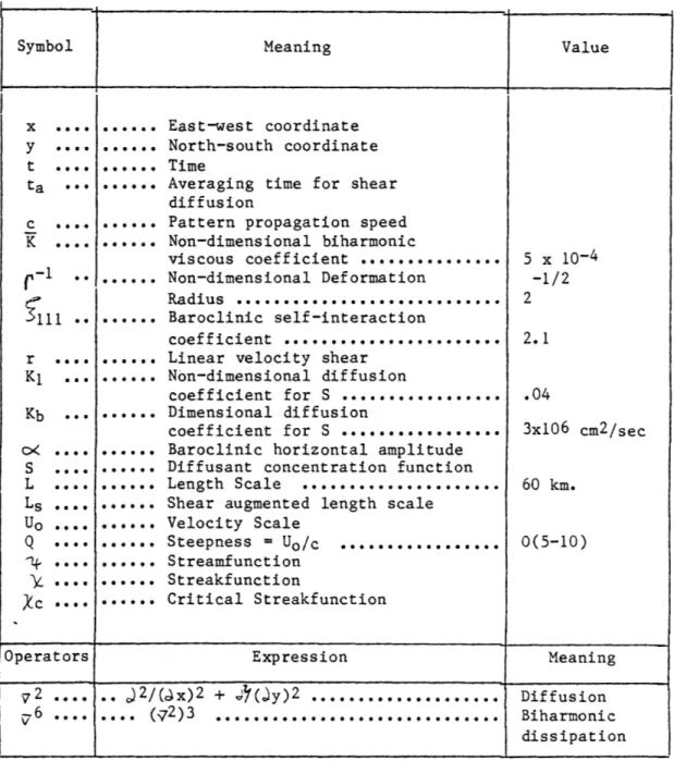
Table III.1 Symbols and Definitions Symbol
::::
::....
.... ... (-1111
r KI Kb o< S L Ls UoQ
Xc
Meaning East-west coordinate North-south coordinate TimeAveraging time for shear diffusion
Pattern propagation speed Non-dimensional biharmonic viscous coefficient ... Non-dimensional Deformation Radius ... Baroclinic self-interaction coefficient ... Linear velocity shear
Non-dimensional diffusion
coefficient for S ... Dimensional diffusion
coefficient for S ... Baroclinic horizontal amplitude Diffusant concentration function Length Scale ... Shear augmented length scale
Velocity Scale Steepness = Uo/c ... Streamfunction Streakfunction Critical Streakfunction Value 5 x 10⁻⁴ -1/2 2 2. 1 .04 3x106 cm2/sec 60 km. 0(5-10)
Operators Expression Meaning
72 .... .. J2/(cx)2 + (iy)2 ... Diffusion 6 .... .... (72)3 ... Biharmonic dissipation I
**
1.
00aa
a0 ••go oo ooo oooo oooo oooo •coo ooo oooo oooo oooo ooo• r ,In order to properly account for the effects of Rings on the various budgets, we must first understand their mass transport properties, and in the present chapter, we will compute the particle trajectories associated with a numerical Gulf Stream Ring. In addition, we will discuss a series of advection-diffusion experiments with a view towards understanding how fluid may be exchanged between the trapped zone and the exterior.
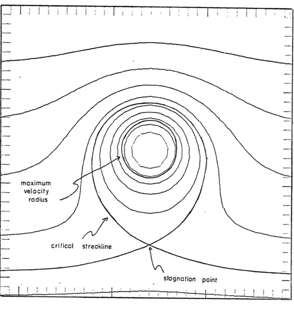
The first theoretical pictures of Ring particle trajectories were obtained by Flierl (1981), in which he computed the streaklines associated with a steadily-propagating, axisymmetric pressure pattern. Trapped zones of fluid, propagating with the Ring, arose in this calculation as a consequence of the strong nonlinearity of the flow. For Rings, the 'steepness', U/c where U is a scale for the particle velocities and c the pattern propagation speed, is of order 10. Outside of the trapped zone, particle trajectories were characterized by meridional excursions on the scale of the Ring (see Fig. III.1). A weakness of Flierl's calculation derives from the fact that his study was purely kinematic. For example, the velocity field he employed, although suggested by data (Olson, 1980), is not a solution to the equations of motion; even though it kinematically resembles a Ring, one must question on dynamical grounds the particle trajectories so
computed. Also, the shape of those particle trajectories do not agree well with those suggested by satellite surface temperature observations. The numerical Ring model we will employ will evolve subject to the conservation of potential vorticity, and therefore will be dynamically consistent. We shall also see that its particle
Figure III.1. Streaklines
Here we have plotted the streakfunction, -K= 4+cy, appropriate to Olson's model streamfunction. Note the critical streakline, stagnation point, and trapped zone. In this figure, the steepness, Q, equals 10; if Q were less than one, all three features would disappear.
trajectories are in better agreement with observations. Still, most of the interesting features of Flierl's analysis will appear in the dynamical Ring, reflecting that his assumptions of steady-propagation and permanent form are apt.
Ring
Model-Many quasi-geostrophic models of Ring structure have been proposed (Flierl, Larichev, McWilliams, and Reznik, 1980) although perhaps the most successful Ring simulations were performed by McWilliams and Flierl (1979). The appealing feature of their model (numerical) is that the
pressure field evolves as a 'monopole', which is in agreement with field observations of the baroclinic structure of a Ring (whether the barotropic component of a Ring also has a monopole character is presently unknown). We will employ their equivalent barotropic Ring model, which was governed by Eq. 11.14:
(02 - p2)lt + Q5111J(,,(2- 12), ) + x = K76~. Eq. 11.14
In the next section, after a brief review of Flierl (1981), we will extend his results to include diffusion. In section c, we will discuss a series of numerical experiments involving the advection-diffusion of a passive tracer by McWilliams and Flierl's dynamic Ring and make comparisons with the previous kinematic results. Finally, we will present some simulations of the often observed Ring/Shelf-Slope Water
III.b Kinematic
Models-Given a steadily propagating streamfunction of the form:
a(x,y,t) = 4(x-ct,y), Eq. III.1
Flierl demonstrated that the streaklines,
<
, of particle motion are given by:S= F+ cy. Eq. III.2
The axisymmetric function:
= UoL(1-exp(-3(r-L)/L)) + UoL/2 r>L
= Uo(x 2
+y2)/(2L) r<L, Eq. III.5
where L denotes the radius of maximum swirl speed, was found by Olson (1980) to accurately describe the streamfunction of Ring Bob, observed during the cyclonic Ring experiment, 1977. Using this function (following Flierl, we will slightly modify Eq. 111.5 by ignoring the '3' in the exponential) in the definition of ~ returns:
X = UoL(1-exp(-(r-L)/L)) + U L/2 + cb r>L a.
Eq. III.$
/<
= Uo(a2+b2)/(2L) + cb = r<L = Uo(a2+(b+cL/Uo)2)/(2L) - c2L/(2Uo) b.Eq. II.4.b is an equation for a circle centered at position (0,-cL/Uo)=(O,Q-1L) relative to the center of the Ring. Clearly, if this point lies within the radius of the maximum velocity, L (i.e.
Q-1<1), those circles close upon themselves, and regions of trapped
fluid will result. The parameter Q=Uo/c, controlling the existence of
closed contours, measures flow steepness and the condition that there be closed contours, Q>1, demonstrates that particle trapping is a kinematic consequence of strongly nonlinear, coherent flow. The finite volume of
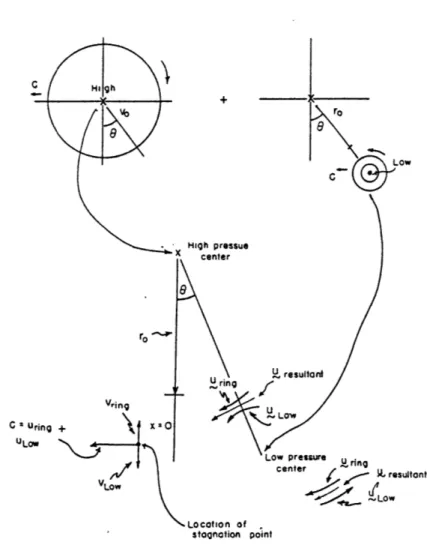
trapped fluid is delimited by a critical streakline, )kc, outside of which the streaklines no longer close. At the apex of Xc is a 'stagnation point' where, in a frame moving with the Ring at speed c, u=0. In a fixed frame, where we perceive the Ring as moving west at speed c, the stagnation point occurs where the fluid velocity identically matches the pattern velocity, ufixed = (c,0).
In Fig. III.1, we plot the streakline contours associated with Eq. 111.4 for a steepness value, Q, of 10, corresponding to a warm Ring propagating westward at a speed of 5 cm/sec with anti-cyclonic swirl speeds of 50 cm/sec. The volume of fluid associated with the trapped zone is roughly three times that of the Ring as defined by the radius of maximum velocity, and the trapped zone shape is asymmetric to the north and south. The equivalent picture for westward propagating cold Rings may be abstracted from Fig. III.1 by switching north for south.
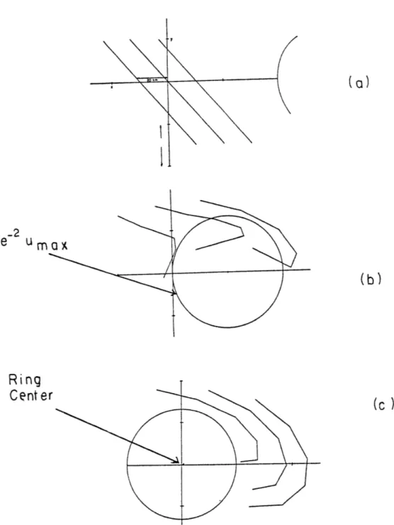
From Fig. III.1, we see that particles just north of the critical streakline are displaced strongly to the north as they move around the Ring, while those near to the northern edge of the Ring undergo much less dramatic meridional excursions. Thus, the fluid develops strong shears near the northern edge of the Ring, which acts to distort material lines of fluid. An example of this is shown in Fig. 111.2, where we plot a history of several material lines as affected by the streakline field in Fig. III.1.
-2
e
U a
Ring
Cent er
(0)
(b)
(c)
Figure 111.2. The Effect of a Ring on Material Lines
Here we demonstrate that, in the vicinity of a Ring, the fluid develops strong shears. We have plotted the relative orientation of three lines at various stages of Ring interaction. In (a), the Ring is far away, in (b), the lines are in the midst of the Ring, and in (c), the Ring has passed. Marked are the Ring center, and the radius where the velocities are e- 2 of their maximum.
Tracer Diffusion in Kinematic
Models-Consider now the problem of advection-diffusion of a tracer S, with the advection provided by the kinematic Ring model of Eq. 111.3. We shall model diffusion according to Fick's law:
Flux = -KbVS,
where Kb is the exchange coefficient pertaining to S. Under these circumstances, the appropriate equation to solve, in the frame of the Ring, is Eq. 11.22, with the advection field given by
7;
St +J(,S) = Kbq 2S. Eq. 11.22
Scaling time by L/c, /. by UoL, and x and y by L, the non-dimensional form of Eq. 11.22 becomes:
St + QJ(X,S) = K172S Eq. III.7
where the steepness number, Q=Uo/c, is of order 10, and K1-1 cL/Kb is a Peclet number. For Kb=0(106 cm2/sec) (Needler and Heath, 1975), K1=(.0 4), thus the oceanographically interesting parameter range corresponds to a weak diffusion/strong advection limit.
Tracer Homogenization on Closed
Streamlines-There are some interesting ramifications of Eqs. 11.22 and 111.7 when applied to regions of closed X(, with regards to the short time evolution of an arbitrary initial condition. An initial point of dispersant imbedded in a linear shear flow, u(x)=rxi, will spread horizontally as:
(Csanady, 1975; Young, 1981). The mechanism involved is shear dispersion, i.e. diffusion spreading the material across the flow, allowing the advection field to enhance the downstream transport. If we suppose that this same shear-augmented diffusion model applies in a local sense, we see that diffusion will tend to force arbitrary initial conditions towards uniformity on closed streaklines. Scaling the shear in the closed X{regions by Uo/L, the spread, Ls, of the initial point source, will become of order L, and therefore nearly uniform over the closed contour, at a time:
ta = (LUo/Kb)1
/3L/Uo. For scales appropriate to Rings, this time is:
ta = [(6x10⁶ 50)/(3x106)]1/3(6x106/50) = 6.1 days.
An exception to this rule occurs for solid body rotation, in which case the time scales are controlled by diffusion:
td = L2/K.
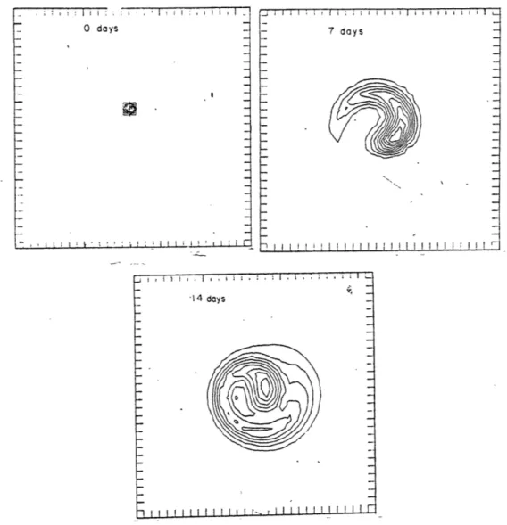
In Fig. 111.3, we present a numerical example where both processes are occurring. In this simulation, velocity shear is concentrated near the edges of the trapped zone, while the center is characterized by a constant rotation rate. Note that by day 14, 0(2ta), the dispersant has homogenized near the edge of the trapped zone, but not in the center. Thus, within the trapped zone, we understand the processes which will act on the dispersant, both of which spread it over the closed contours, and in the presence of shears, force it towards homogeneity along
7.
Therefore, with little loss of generality, we have chosen initial conditions like S(x,y,t=0) = f() for those advection-diffusion experiments in which the initial blob was located inside the trapped zone.O days
14 days
I I It I I I I I
r
Figure 111.3. An Example of Tracer Homogenization
Here are the results of a numerical integration of Eq. 111.7, using 7as shown in Fig. III.1. Note that this velocity field is composed of solid body rotation out to the maximum velocity, followed by an exponential decrease. All of the shear in the velocity field is located near the critical streakline, and it is there that the tracer has homogenized. In the region of solid body rotation, the time scale for homogenization is the diffusive time scale, which is a much slower process. _..I J i I , 1 II i i I II i i i - 7 days _ _ -?_ 1 I I ! 1 T ! ] 1 I I [ I I ! ! ! 1 i i 1 ! I r V i ' i . . . . .