Asymptotics of Wavelets and Filters
by
Jianhong (Jackie) Shen
Submitted to the Department of Mathematics
in partial fulfillment of the requirements for the degree of
Doctor of Philosophy
at the
MASSACHUSETTS INSTITUTE OF TECHNOLOGY
June 1998
@1998 Jianhong(Jackie) Shen
All rights reserved
The author hereby grants to MIT permission to reproduce and to distribute publicly
paper and electronic copies of this thesis document in whole or in part.
Author ...
Department of Mathematics
May 1, 1998
Gilbert Strang
7
rofessor of Mathematics
Thesis Supervisor
Accepted by....
,hairma
Hung Cheng
Applied M
aema
s Committee
Accepted by...
Richard B. Melrose
Chairman, Department Committee on Graduate Students
of-
H-NOIT '"JUN
011i8
Science
LIBRARIES
by
Jianhong (Jackie) Shen
Submitted to the Department of Mathematics on May 1, 1998, in partial fulfillment of the
requirements for the degree of Doctor of Philosophy
Abstract
In Wavelet Theory, the most significant (both historically and in the present stage) family of wavelets is the Daubechies orthogonal wavelets with compact supports. The most powerful source of curiosity and imagination is the key equation-the Refinement Equation (or Dilation Equation). And finally, it is the keyword "filter" that has served as the major bridge connecting mathematicians, physicists, and engineers, and made Wavelets Theory one of the very few examples in this century that was rooted in several different fields, and was someday unified in the paradise of mathematics (Harmonic Analysis and Approximation Theory), and eventually found itself in the broad market of engineering fields (especially in the information processing technology). This thesis is a mixture of my research results on analyzing, generalizing, and developing Daubechies family of orthogonal wavelets, the Refinement Equation, and the design of digital filters. The main tool is asymptotic analysis.
To study Daubechies' family of wavelets, we first study the associated Daubechies lowpass filters (or polynomials). The distribution of zeros is closely studied and its asymptotic pattern is obtained. The transition bandwidth of the filter is found to be proportional to the inverse of the square root of the number of zeros at the "highest" frequency w = r (a key number also determining the smoothness of the wavelets). This first step breaks the secret of the nonlinear phase information of the filters. The leading linear term approximation of the phase makes it possible to carry out asymptotic analysis on Daubechies wavelets and scaling functions. The energy significant parts of the wavelets and scaling functions are determined by the stationary phase method.
Our study of the Refinement Differential Equations (RDE) was the first one in the literature. It is motivated by a perturbation of the Refinement Equation and the search for wavelets-like functions. We establish the connection between wavelets and solutions to certain types of functional differential equations, a hot topic near 1970s. We reveal the general structure of solutions to RDE's and discover that RDE's are naturally connected to a class of Refinement Functional Equations (RFE). The Continuous Subdivision Algorithm finds its dominant place in solving RDE's. The vague probability idea of Rvachev (1971) is developed more completely.
In spite of the simple formulation of various (weighted or unweighted, real or complex domains, simply connected or multiply connected domains) Chebyshev (L') polynomial approximation prob-lems, the analytic behavior of solutions remains a mystery except for some simple cases, due to the lack of geometric structures. This is the underlying reason why engineers working on filter designs are frequently puzzled by certain behaviors of optimal filters. Based on Fuchs' work, we improve and interpret a widely-used empirical formula established by Kaiser based on his numerical data in 1972. Our new asymptotic formula proves to be more accurate than Kaiser's. To compute the critical constant (related to the Green's function of the underlying domain), we study properties of the Green's function for a multi-interval domain as well as its equilibrium distribution measure. This result also contributes to the numerical analysis of partial differential equations (the Stokes equation in fluid dynamics, for example).
Thesis Supervisor: Gilbert Strang Title: Professor of Mathematics
Credits
Most of the material in this thesis has appeared or will appear in some journals, or has been submitted. The work on Daubechies filters, scaling functions, and wavelets in Chapter 2 is joint work with Gilbert Strang. The analysis and computation of the zero distribution appeared in [65, 1996], and the asymptotic analysis of the scaling functions and wavelets will appear in [66, 1998]. I would like to thank Cleve Moler (MathWorks Inc.) for providing his numerical observations. The material in Chapter 3 has been submitted [64, 1997] and presented in the 9th International Conference of Approximation Theory. I would like to thank Gilbert Strang and Dingxuan Zhou (Hong Kong City University) for introducing me Rvachev's work in 1970s and providing useful references. The material in Chapter 4 is partly joint work with Gilbert Strang and will appear in [67, 1998]. The newest parts [68, 1998] are now developing from a conformal mapping idea of Nick Trefethen (Oxford Computing Lab). I would like to thank Alan Oppenheim (MIT EECS) and Jim Kaiser (Bell Lab) for discussing REAL problems in the design of digital filters.
I would also like to thank the many people who have made useful suggestions to me in my research. Among them, I would especially mention Tomas Arias, Dmitri Betaneli, Hung Cheng, Ingrid Daubechies, Alan Edelman, Ross Lippert, Truong Ngyuen, Alan Oppenheim, Gilbert Strang, Vasily Strela, Nick Trefethen and Andy Wathen.
Acknowledgement
I would like to express first my abstract but deep appreciation: to the ancient Chinese philosophy and tons of wisdom stories in her history - making me aware of the importance of "being balanced" in every aspect of my life; to the great man Deng Xiaoping - Lincoln liberated millions of slaves of USA, while Mr. Deng has set free a billion of heads in China (and mine is one epsilon among them); and finally, to the United States, for her generosity and kindness to foreigners, and her spirit of being mixed, not to chaos, but to the benefits of all our human beings.
I also feel deeply inside that I owe each person in the department a "thank you", for their friendly helps and daily "hello"s, with which, I found my big family in the USA. Especially, I would like to thank Linda, for her candies and cookies in Room 233, where, consciously or not, I loved to drop by, and for her heart-shaped Valentine Day cards to every graduate; and Shirley, Sueli, and Nini, with whose "universal" keys, I never worried about being locked out of my office; and Eda, for each of her heart-warming emails reminding our proctoring assignments; and Tivon- my personal calls made in the headquarter could never be free :-( , yet personal faxes for me always reached me so timely :-).
I am also grateful to those in the department who have taught me mathematics and academic skills: to Greenspan and Malkus, for introducing me to the world of fluid mechanics and solar dynamos; to Edelman, for the influence on me of his love of numerical linear algebra (and his one summer support, which was so important to me as a foreign student); to Stroock, for teaching me the beauty of theoretical probability and Martingale theory; to Toomre -being his TA on numerical analysis was the most unforgettable experience in the past four years. I owe special thanks to Hung Cheng, with whom I can speak Chinese and express more personal feelings about the new life here, not mentioning his teaching me on integral equations and asymptotics of ODE's. To complete my moral payment, I would like to thank Gian-Carlo Rota, from whom I learned the beautiful classical theory of polynomials, umbral calculus, exterior algebra, Clifford algebra, and invariant theory, as well as the "stories" or "philosophy" behind them; and from whom I learned how to be persistent in research, and how to create something from nothing.
Acknowledgment
Betaneli, Peter, Mats, Lior, Mathew, Radica and Lisa. To me, they were the most helpful dictionaries when I could not figure out an English word or wanted to know a certain side of the western life; the most enjoyable group of people talking with either about a small funny thing I discovered or a homework problem.
I would like to thank all my Chinese friends in the department: those still here or having graduated. Besides mathematics and speaking English, speaking Chinese was so important a part of my daily life. When words are merely symbols, feelings can be evaporated. But when words are feelings, then to speak is to touch, to express, to enjoy, and to generate solutions to every hard problem in life. I don't know how to weigh the importance of a native language and native friends. I would also like to thank especially my chinese friends in other departments, who have had great influence on my life. Among them, I would like to mention Chuan He, Wen Zhang, Qiang Zhu, and Shanhui Fan. We approximate each other to a very high precision in many sides of our personality and academic styles. The lunch table was a constant source of jokes and knowledge. I cannot imagine a life without them. I really felt it a privilege talking about the protein folding problem when our girlfriends were hunting in Macy or Sears for their suits. And my words feel too powerless to take a photo of my happy time, sitting together with them on the lawn of Boston Botany Garden in the fresh spring time, playing cards from dawn to sunset.
I have benefited greatly from my practicing of teaching for more than two years at the Tutoring Room Service, and the Experimental Study Group at MIT. Special thanks must also go to the Wellesley College for offering me one semester of teaching job. Also allow me to thank the Graduate Student Council of MIT for supporting me in the 1998 AMS annual meeting.
Finally, I feel I can never pay back to my advisor Gilbert Strang and my closest friend Tianxi Cai. They have defined my well-balanced and happy academic life and "plain" life, on this land far away from my family and homeland. let me dedicate to them the following famous poem by Bo Wang (Chinese, 650-676) (hope my translation is an isomorphism, of both words and thoughts):
Where there are seas and lands, there are those knowing you,
as deep as yourself to you... there are those with you,
Contents
1 On Asymptotics 1
1.1 What Is Asymptotics ... ... . 1
1.2 Examples of Asymptotics ... ... 2
1.3 Mechanisms for Asymptotics ... ... 5
1.4 Introduction to the Thesis and Its Asymptotic Contents . ... 6
2 Asymptotics of Daubechies Mini-phase Filters and Wavelets 8 2.1 The Zero Distribution of Daubechies Filters ... 9
2.1.1 Introduction ... ... 9
2.1.2 A Note about the Numerical Computation of Zeros . ... 11
2.1.3 A Clue from the Three-term Recursive Relation . ... 12
2.1.4 Two Bounds for the Zeros of Bp(y) ... ... 14
2.1.5 Regular Zeros and Singular Zeros ... .. ... . . 17
2.1.6 Transition Bandwidth ... ... 21
2.2 Asymptotics of Daubechies Mini-phase Wavelets ... . 22
2.2.1 Introduction ... ... .. 22
2.2.2 Accuracy of Approximations ... ... 25
2.2.3 Fourier Integrals with Large Parameters ... . ... . 30
2.2.4 Asymptotic Structure of bp(t) and ,p(t) ... .. ... . 34
2.2.5 Asymptotic Structure of Wavelets ... ... 38
2.2.6 Asymptotic Structure of the Filter Coefficients . ... 39
3 Refinement Differential Equations and Wavelets 43 3.1 Introduction ... ... . ... 44
3.2 Regular Equations and the Structure Theorem ... ... . . 47
3.4 General Regular RDE's . . ...
3.5 Distributions and Refinement Functional Equations . . . . 3.6 Probability Method and Continuous Subdivision Process . . .
3.6.1 Probability Method . . ...
3.6.2 Continuous Subdivision Scheme for Generic RDE's . . 3.7 Application: Smoothed Wavelets and Quasi-Multiresolution . 3.7.1 Classical Wavelets with Compact Support . . . . 3.7.2 Smoothed Wavelets and Quasi-Multiresolution . . . . 3.7.3 Smoothing versus Small Deviation . ...
4 Asymptotics of Optimal Lowpass Filters
4.1 Asymptotics of the Error-Length Relation . ... 4.1.1 Introduction . . . ...
4.1.2 Leading Order For 6 . . ... 4.1.3 The Symmetric Case . . ... 4.1.4 The General Case . . ...
4.1.5 Kaiser's Filters Are Near Optimal . ... 4.1.6 Numerical Experiments . ... 4.1.7 The Transition Band . . ... 4.1.8 Appendix . . . . ...
4.2 The Green's Function of Several Intervals and Its Asymptotic 4.2.1 Introduction . . . ...
4.2.2 The Green's Function for Two Intervals . . . . 4.2.3 The Green's Function for Several Intervals . . . . 4.2.4 Applications of the Square Root Law . . . ... 4.3 The Equilibrium Distribution and Asymptotics of Extremal F
4.3.1 4.3.2 4.3.3
The Potential and Equilibrium Distribution ... . Asymptotics of Extremal Points and Its Applications Summary . . . ... .. . . . . 61 .. . . . . . . 64 . . . . . . . . . . . 69 .. . . . . 69 . . . . . . . . . . . 74 . . . . . 78 .. . . . . 78 . . . . 80 .. . . . . 81 85 ... . . . . . 86 ... . . . . . 86 ... . . . . 88 .. . . . . 90 .. . . . 92 .. . . . . 96 .. . . . 97 .. . . . 99 . . . . . . . 102 s . . . . 104 . . . . . . . 104 . . . . . . . . 109 .. . . . . . . 113 . . . . . . . 117 'oints ... 120 . . . . . . . 120 . . . . . 123 . . . . . . . 125
Chapter 1
On Asymptotics
1.1
What Is Asymptotics
There are many textbooks and conference procedings on asymptotic analysis and its applications. But none of them has given an overall synthesis on this subject, or has updated the content of asymptotics. In this first chapter, I give my attempt. Though asymptotic analysis is only one tool in my thesis (not the subject), I still feel it valuable to freshen and broaden our viewpoints on this old but never dormant subject, because the way we view thiilgs, determines the way we act and justify our actions. Also the discussion of general asymptotics may provide some important background for this thesis.
Almost all asymptotic analysis textbooks consist of three major parts: how to sum infinite series, how to evaluate integrals with large parameters (Laplace or Fourier types), and how to solve differential equations with a small or large parameter (second order differential equations typically). They are three major columns for the hall of classical asymptotic analysis. But to me, asymptotic analysis has already been scattered in several fields: classical analysis, probability, combinatorics, dynamic systems, and so on. It depends on our understanding of the meaning of "asymptotics", and in the following I have chosen bravely the widest (and therefore maybe wildest) one.
Using the least number of words, asymptotics means trends.
What studied by asymptotic analysis is a system of objects. It can be a family of integrals or differential equations, or a sequence of polynomials, or a dynamic process (such as matrix iterations in numerical linear algebra and iterations of maps in a dynamic system), or a collection of random variables. In any case, the target objects must be connected by at least one parameter, which can be either the real time (as in differentiable dynamic systems), or a discrete "time" (as in various
iterations), or a crucial system parameter (such as the number of vanishing moments for Daubechies family of wavelets with compact supports, the size of a gap between two close intervals, or a dimen-sionless physical constant in differential equations). The central task of asymptotic analysis is to detect and classify trends of the systems as the parameters vary (especially toward some extremal values), to predict the "speed" (temporal) or the "scale" (spatial) of the trends and to give simple but practically useful approximations to the trends. Therefore asymptotic method is one among a handful of powerful "applied" methods.
1.2
Examples of Asymptotics
An ancient Chinese poet wrote: "you cannot see the real face of Mount LuShan 1, only because you are on it." The same applies when we observe a system of objects. You cannot feel the trend of a system unless you allow the system parameter to vary in a very large range ("watch it from a distance"). The behavior of any individual object is often hard to understand, not transparent to analysis, and even unpredictable -- because its behavior is the mixed effect of many factors, and many relations that can be random or deterministic, and linear or nonlinear. Only in the asymptotic case, one can consider only very few dominant factors or relations. This can make things much simpler than usual.
Let us look at several examples scattered in different contexts.
Riemann-Lebesgue Lemma The first simple example is the Riemann-Lebesgue Lemma in anal-ysis. Let f(x) be any L1 integrable function on [a, b] (either a or b can be oo). Then
lim ezAX f(x) dx = 0.
For each individual A, the integral obviously depends on f(x), a and b, and its exact evaluation can be very hard (except by numerical methods). The Lemma captures such a simple asymptotic behavior universally shared by this (Fourier) type of integral. It provides a simple necessary condition for a function to be the Fourier or Laplace transform of an L1 function. In the Riemann-Lebesgue Lemma, the asymptotic trend is the cancellation. The parameter A is the frequency of canceling periods.
Law of Large Numbers and Central Limit Theorem The second familiar example comes from probability. For one ideally random toss of a coin, the result of being head or tail is unpredictable.
1
On Asymptotics
However, after tossing it for many times, "almost surely", for nearly half of the times we must get heads and for the other half, tails. This half to half behavior is an asymptotic one and the parameter is the number of tosses. Generally, this example is summarized by the celebrated Law of Large Numbers, and the Central Limit Theorem describes even more detailed asymptotic behavior. These two fundamental theorems of probability are both asymptotic results. They describe the universal asymptotic behavior shared by a fairly large class of random events. In this example, asymptotics is the sibling of another familiar word: statistics, and basically, the trend is still cancellation or averaging-an individual random variable X is usually complicated, yet asymptotically, there is a lot of cancellation in the independent sum (X1 + X2 + -.. + XN)/N.
Attractor, Ergodicity and Ergodic Theorem The third example is from dynamic systems. In a differentiable dynamic system (on a compact manifold, say), the evolution of an individual state or phase often allows a very wide degree of freedoms and therefore usually has no simple closed form. Fortunately, asymptotically, or as the counting time goes to infinity, the trajectory must exhibit certain universal behaviors such as being attracted by an attractor (or a "sink"), which can be either an attracting state, or a stable limiting circle (mostly in the plane phase case), or even a strange attractor (in a high dimensional phase space). Each flow can be complicated, yet its asymptotic behavior can be simply identified and classified. Another asymptotic example in dynamic system is the set of concepts like "ergodic", "mixing", and "exact". Each of them describes one typical sort of asymptotic behavior of the semigroup generated from the iteration of a given map. The celebrated Birkhoff's Ergodic Theorem is yet another asymptotic example in dynamic system and it is more or less related to the Central Limit Theorem, whose asymptotic meaning is just discussed above.
Regular and Singular Perturbation The fourth example, which is more classical, is the pertur-bation method of linear or non-linear differential equations. Even for second order linear ordinary equations, except for some simple valuable cases such as Cauchy equations, equations with constant coefficients, and equations with analytic coefficients, there is no closed form for the solutions. For-tunately, in application, the dimensionless equation obtained from a physical system often contains a large or small parameter. This usually makes the problem much simpler since the leading terms of the solution can be easily obtained by regular or singular perturbations (though the problem of matching is usually non-trivial). For example, the (leading term) solution to the following equation containing a small parameter
can be easily found by solving one first order outer (or slowly varying) problem and two second order inner (or boundary layer, or rapidly varying) problems. In this example, the asymptotic means the trend of spatial variation: as c gets smaller and smaller, the region with rapid spatial variation tends to be more and more concentrated near one of the boundary points-the famous phenomenon of
boundary layer.
Polynomial Sequences The last example concerns polynomial sequences. Let us consider two classes of polynomial sequences that are closely related to Chapter 2 and Chapter 4 in this thesis. The first class is the partial sum sequence of the power series (at some point) of a meromorphic function. For example,
Z2 Z
n
q,(z)= 1+z+ + +
-2! n!
for ez at z = 0. A question asked and answered by Szeg6 is the zero distribution pattern of qn(z). It is hard to describe precisely the zeros of qn(z) for each individual n (except for n = 1, 2, 3, 4). However, asymptotically, the zeros of q, (z) behave very regularly-after a simple elementary trans-form, the zeros are nearly equidistributed along the unit circle. And this asymptotic pattern is universally shared by this class of polynomial sequences. The second class of polynomial sequences are Chebyshev polynomials for a domain and a given function. That is, given a function f(z) and a domain K in the complex plane, p,(z) minimizes the error
11f - Po IIL (K)
among all polynomials of degree n. The behavior of p,,(z) obviously depends on f(z), which can be very complicated and arbitrary: entire, meromorphic, analytic, smooth, or only continuous. Besides, the domain can also have a large degree of freedom. However, as the approximation order gets larger, the sequence always exhibits certain common asymptotic behavior. In Chapter 4, we
study the asymptotic behavior of a polynomial approximation problem from digital filter design. Summary These examples are scattered in different fields and have never been seen via a unified viewpoint. The purpose of of the listing is to extract something common hidden in them and therefore to find a quasi-foundation and methodology for them.
On Asymptotics
1.3
Mechanisms for Asymptotics
If we are the loyal followers of the cause-effect philosophy, there must exist some common causes leading to asymptotics or trends. These causes, or "forces" as I would like to call in the following, in my opinion, include the following three major ones: cancellation, averaging, and attraction. Cancellation The cancellation mechanism sees itself in the Riemann-Lebesgue Lemma, the method of Stationary Phase, and even in the Law of Large Numbers. We can understand it in the following quasi-philosophical way. Inside each object of a given system, there is more than one force (typically two, Yin and Yang, for example). Those forces are not balanced in an individual object because of random factors, and thus make the individual objects varying and complicated. Those objects are linearly ordered according to a certain system parameter (frequency, say), which more or less characterizes the cancellation degree of those forces. As the parameter increases, the cancellation gets stronger and certain steady (or stationary) trends can appear. This is the asymptotics arising from cancellation.
Averaging The averaging mechanism to asymptotics appears in the Law of Large Number, the Central Limit Theorem, and the Birkhoff Ergodic Theorem. It is more or less associated to statistics. The asymptotic or trend in this case is obtained from averaging a large sample of objects. The individual irregularities cancel out each other during the averaging process. In this case, the objects of the system must carry certain degree of randomness or diversity. For example, the iterations of an ergodic map must be able to send any non-zero mass almost everywhere. In signal processing, averaging means the elimination (or filtering) of high frequencies. Asymptotic trend is usually steady and stationary, and therefore corresponds to low frequencies. They are preserved and even amplified during the averaging (lowpass filtering) process.
Attraction Attraction is probably the most common way leading to asymptotics or trends. Unlike cancellation, whose mechanism depends on two or more internal forces, and averaging, which requires certain degree of randomness from the system, attraction is caused by certain deterministic "external forces." The simplest example is the iterations of an initial state under a contracting map. The "external force" is the contracting mechanism, which for a linear system, is usually caused by the spectral radius of a linear operator (less than 1). The "external force" is also the unique fixed point (suppose the metric space is complete) in the sense that the trajectory of any initial state is attracted to it. Sinks, limiting circles, and strange attractors are more examples of "external forces." 2
2
Let us enumerate more examples. Consider the classical one:
j
e-Af
(x)
dx,
where A is a positive parameter. Suppose f(0) is not zero (and assume f is smooth for simplicity). Then the leading term as A gets very large is simply f(O)/A. It is obtained by replacing f(x) by f(0) in the integral. As A gets larger, the effect of x = 0 becomes more and more dominant. It acts like a strong force pulling the whole weight of integration round it.
Also consider the boundary layer phenomenon. In this case, fluid mechanics leads to a more vivid picture of the "external force"-the drag of a plate or some boundary material to the liquid. As viscosity gets smaller (or the Reynolds number gets larger), the propagation of this influence through shear stress of the liquid is more confined near the boundary and we observe thinner boundary layers. Finally, let us look at the asymptotics of the zeros of the partial sum polynomial sequence of a meromorphic function. The scaled zeros will converge to a limiting curve (see Chapter 2, for example), which acts as an attracting force. In fact, the underlying mechanism for this attracting force is exactly the same as that discussed in the second paragraph.
Summary The understanding of asymptotic mechanisms helps us to adopt appropriate methodol-ogy in applications. For attraction, the main task of asymptotic analysis is to identify the "dominant force" and find a suitable approach to amplify its influence. For averaging, it is often inevitable to turn to the methodology of statistics and operator theory. For cancellation, it is crucial to locate the states where cancellation is the least (since they will determine the leading terms).
1.4
Introduction to the Thesis and Its Asymptotic Contents
Chapter 2 studies the Daubechies miniphase orthogonal wavelets with compact support (for spline wavelets, the work has been carried out by other people). The major difficulty of analyzing this family is caused by the complicated non-linear phases of the associated filters. The wavelets also have the same property-with simple magnitudes but very complex phases (in the Fourier domain). From a certain angle, this family of wavelets is very alike the Airy function, whose Fourier transform is also purely phased. Our analysis starts with the asymptotic pattern of the zeros of the filters and ends at the asymptotic structure of the wavelets. Basically, the asymptotics of a polynomial sequence (derived from truncating the power series of a family of meromorphic functions) and the method of stationary phase are used in this chapter.
On Asymptotics
In Chapter 3, we study a generalization of the Refinement Equation. A refinement equation has the following form
O(x) = h[0]4(2x) + h[1]¢(2x - 1) + ... + h[N]¢(2x - N)
for some real coefficients (or filter coefficients) h[O], .. , h[N]. The Refinement Equation plays a crucial role in the theory of wavelets with compact support. It also links Wavelet Theory to signal processing and other fields. After perturbing this equation, we obtain a new class of equations called Refinement Differential Equations. Our major achievement in this chapter is the discovery of the link of Wavelet Theory to the theory of functional differential equations and probability theory. This chapter contains the least content of asymptotics, however.
Chapter 4 studies a particular polynomial approximation problem arising from digital filter de-signs, and also the associated potential theory for a several-interval domain. The asymptotic behav-ior of the optimal polynomial sequence is often determined by the singular locations of the target function (i.e. poles) and the critical points of the Green's function for the working domain (the "external forces" mentioned in the preceding section). The first part impoves an empirical formula discovered by Kaiser regarding the relation of optimal errors to filter lengths. The second part studies the Green's function and equilibrium distribution of a several-interval domain based on the Schwarz-Christoffel mapping. Both structural and asymptotic results are established.
Asymptotics of Daubechies
Mini-phase Filters and Wavelets
Though it now has been a clich6 - "to analyze wavelets, first analyze the filters," it never hurts in practice to follow this simple principle.
The first part of the chapter studies the asymptotic behavior of Daubechies filters (polynomials). The zero distribution pattern of the filters is crucial in their filtering effects as well as in the next stage of analysis (on wavelets). Here the objects are discrete (polynomials and their zeros), yet the result is continuous (the existence of the limiting curve). The second part studies the asymptotics of Daubechies scaling functions and wavelets based upon their Fourier integrals. The stationary phase plays an important role here. In this part, the objects are continuous (integrals and wavelets), yet the result is in certain sense discrete (three different scales with separate asymptotics).
Asymptotics of Daubechies Filters and Wavelets
2.1
The Zero Distribution of Daubechies Filters
2.1.1
Introduction
The Product Filter P(z): Positivity and Zeros
Let H(z) =
E'
0 h[n]z -n be a lowpass filter whose associated Refinement Equation N0(t) = h[n]q(2t - n)
n=O
yields orthogonal integer translates {(t - n) I n E Z}. Its associated "energy" filter, or the product
filter P(z) is defined by P(z) = H(z) - H(z- 1) . In order that the integer translates of the scaling function are orthogonal to each other, it is necessary for H(z) to be a quadrature mirror filter
(QMF), a connection first made by Mallat. This means
P(z) + P(-z) = 1. (2.1)
Such a filter is called a halfband filter. Its impulse response h[n] is always zero at even times n = 2k except when n = 0.
The product filter has the following two remarkable properties: (1) Positivity: P(z) > 0, for all
jzj
= 1.Suppose z = e". Then H(z - 1) = H(z) and P(z) = IH(z)2 > 0. Combined with the
symmetry property P(z) = P(z-1), we conclude that P(z) must be a nonnegative polynomial of x = cos w:
L 1
p(x) =Z:c[nlx', p(x)=P(± 2
n=O
(2) Zeros at z = -1.
Since H(z) is a lowpass filter, we always impose the lowpass condition: H(1) = 1. Then
P(1) = 1 and Eq.(2.1) implies: P(-1) = 0. Therefore P(z) must have zero(s) at z = -1, or the highest (digital) frequency w = 7r. This, in return, implies H(-1) = 0.
There is a profound influence of those zeros at z = -1 in Wavelet Theory. As shown in Battle [3, 1989], Mayer [50, 1992], Daubechies [10, 1992], and their most recent improvement in Cai and Shen [7, 1998], those zeros are necessary to achieve good smoothness for the wavelets. If an orthogonal wavelet is Cm , then at least m zeros of H(z) should be guaranteed at z = -1 (even more in practice).
Whereas image processing engineers debate the real necessity of smoothness in their applications, mathematicians feel no hesitation to have it - for the purpose of regularity analysis of functions and having "good" basis functions for the Wavelet-Galerkin method (for solving PDE's numerically).
A general design problem of orthogonal wavelets starts with the design of P(z). The number of zeros at z = -1 must be an even number, say 2p. It is therefore convenient to factorize it in the following form:
P(z)= +Z1) (+Z)PQ(). (2.2)
Obviously Q(z) must also be nonnegative on the unit circle and have a symmetric impulse response. It is the Q(z) part that has induced the diversity of orthogonal wavelets with compact supports.
Ingrid Daubechies chose Q(z) in a typical mathematician's way: Q(z) is extremal in certain sense.
Daubechies' Maxflat Condition
The Maxflat Condition asks for the lowest order of Q(z) such that P(z) defined by Eq.(2.2) is both a halfband filter and nonnegative when restricted on the unit circle.
It is convenient to introduce another variable y: y = (1 - x)/2. Here x = (z + z-1)/2 is the
Joukowski transform ( x = cos w when z is restricted on the unit circle). Since Q(z) is symmetric, it must be a polynomial of x, and therefore of y. Denote it by B(y). Then p(y) = (1 - y)PB(y), if
p(y) denotes the "y-transform" of P(z). The halfband condition Eq.(2.1) now becomes
(1 - y)PB(y) + yPB(1 - y) = 1. (2.3)
Notice that y E [0, 1] as z changes on the unit circle. Therefore mod yP,
(1 - y)PB(y) - 1,
or
B(y) (1 - y)P 1 + py + y2 3
(1 y)P (- 2 3
Define B,(y) to be the following polynomial of degree p - 1:
S
+1y2 +p-1. (2.4)Asymptotics of Daubechies Filters and Wavelets
Then B(y) = Bp(y), mod yP. This means the lowest order of B(y) can be p - 1. And it is not difficult to see that p(y) = (1 - y)PBp(y) is the unique Hermitian interpolation polynomial of degree
2p - 1 that interpolates 1 at y = 0 and 0 at y = 1 both to order p. By symmetry, p(y) must satisfy the halfband condition Eq.(2.3). Therefore Bp(y) is indeed the polynomial with the lowest degree. Daubechies made this choice. Various Daubechies families of wavelets have been designed from it. The difference lies in the procedure of factorizing P(z) into a product of H(z) -H(z - 1) (the
so called spectral factorization). In this thesis, we only demonstrate the most natural factorization: the mini-phase spectral factorization, which leads to the mini-phase orthogonal wavelets.
To start, suppose we have already known the p - 1 roots Y, Y2, '" , Yp- 1 of Bp(y). By the rule
of Joukowski transform z + z- 1/2 = 1 - 2y(= x), in the z-plane, we have 2p - 2 preimages of those Y,'s-exactly half of which lie inside the unit circle. Denote them by Z1, Z2
,...
, Zp- 1. Then theDaubechies mini-phase filter is defined by
H( 1 + z- 1 p -1 1- Z-1Zn
H(z)
Z
1- Z (2.5)n=l
If the product factor is omitted, the Refinement Equation produces spline functions-with accuracy
p but not orthogonal to their integer translates.
Our main goal is to analyze the zero distribution pattern of Hp(z).
2.1.2
A Note about the Numerical Computation of Zeros
Before we set out applying many analytic methods, let us first mention briefly the numerical com-putation of the zeros using Matlab, a popular software for signal processing and wavelet analysis.
Matlab creates the companion matrix whose characteristic polynomial is B,(y). Then it finds the eigenvalues of that matrix. Without scaling, this breaks down at p = 35, because of the wide range in the coefficients of Bp(y). The first coefficient is 1, and by Stirling's formula, the coefficient of yp-1 is
(2p
- 2) /27(2p - 2) (2p - 2)2p-2 4P-1p- 1 2r(p - 1) (p - 1)2p-2
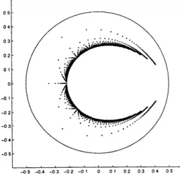
The leading term 4p - 1 suggests that the variable 4y is preferable to y. With this scaling, the Matlab computation remains accurate to p = 80. For larger p, a bifurcation (see Figure 2-1) occurs from roundoff error. The coefficient (P-'+i)4-i of (4y)i is numbered b(p - i) by Matlab. Then b(p) = 1
and the sequence of coefficients is created recursively;
fori= p- 1: -1: 1, b(i)= b(i+1)*(2p-i- 1)/(4*(p-i)); end
The command "Y = roots (b)/4" produces the approximate zeros Y(1),..., Y(p - 1).
Figure 2-1: A bifurcation occurs from roundoff error, p = 100.
Experiments with other root-finding algorithms were less successful, even though working with the companion matrix is a priori surprising. A polynomial with repeated roots leads to a defective matrix (not diagonalizable). Algorithms based on Newton's method had difficulty with the accurate evaluation of Bp(y) and B,(y). Lang's algorithm (Lang and Frenzel [45, 1994]) is comparable to Matlab 'roots', and probably faster.
2.1.3
A Clue from the Three-term Recursive Relation
In this section, we attempt to have a clue of the zero distribution pattern of Bp(y) from its recursion formula.
From Eq.(2.4),
B 1 + py + 2 1y2 ... + p-1
p- 1
yB, = y + py2 + .p. .+ 2p -3)Y-1 +p(2p, - 2) YP.
(p-2 p-1
Hence
(1- y)Bp = Bp- 1 + (2p3) P- (1 - 2y).
Asymptotics of Daubechies Filters and Wavelets Since
(
2p - 1\ p-1} 2p - 3\ (2p - 2)(2p - 1) _ 1 2p- 3 p-2 p-23 ( (- (-1)p )p -2(2- p) \p-2 - ' by setting c, = 2(2 - p-1), we have(1 - y)B+l1 - [1 + cpy(1 - y)]Bp + cpyBp_1= 0. (2.7)
Note that c, -+ 4 as p --+ co.
Lemma 1 Suppose a sequence of meromorphic functions fp(y), p = 0, 1, - -- satisfy the following three-term recursive relation:
(1 - y)f,+l (y) - [1 + 4y(1 - y)]
f,(y)
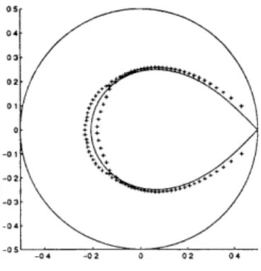
+ 4yf,_l(y) = 0.Then generically as p -+ oc, zeros of fp(y) in the holed complex y-plane C\{0, 1, o00 approach the following lemniscate (see Figure 2-2):
14y(l - y)j = 1.
Figure 2-2: Zeros of Bp(y) approach the lemniscate: 14y(1 - y)I 1. Proof. The auxiliary equation (AE) for the recursion formula is
(1 - y)A2- [1 + 4y(l - y)]A + 4y = 0.
Since y changes, A is a function of y. It has two auxiliary roots:
1
A 1= - 2 = 4y.
Therefore
fp(y) = A(y)A'(y) - B(y)A'(y)
for some suitable coefficients A and B (both depending on y). In fact,
fI - fOA2 f1 - f0 1
A= B=
AA - A2 B 1 A2-
By "generic", we mean both A(y) and B(y) are not zero functions. Since fo and fi are meromorphic functions, so are A and B. On the zero set of f,(y), we have
[A2]P A A, -. B '
or
14y(1 - y) = JA2/Ai = IA/BI I p.
If A/B = 0 or oo, A2/A1 = 4y(l - y) = 0 or oo. This is only possible when y = 0, 1, or oo. On the
rest of the y-plane, IA/B I is finitely positive. Hence JA2/A1| approaches 1 as p -- o0. Oi
This lemma gives us a clue of how the zeros of Bp(y) might behave in the complex plane. However, since cp is not exactly 4, we cannot apply it directly to Bp(y). It seems that we have to analyze Eq.(2.7) through perturbing the three-term relation in the lemma. The analysis then gets very involved. We therefore abandon this method and turn to a more analytical and easier method first used by Gabor Szeg5.
Let me mention that there is no reason to curse the non-zero 4 - c, = 2p-1 . It is this small deviation that makes the sequence Bp(y) a polynomial sequence. Generally fp(y) can be at most a sequence of meromorphic functions.
2.1.4
Two Bounds for the Zeros of BP(y)
In this section, we prove two bounds for the zeros. Let Y denote an arbitrary zero of B,(y), and Z any preimage of 1 - 2Y under Joukowski transform.
Asymptotics of Daubechies Filters and Wavelets
Theorem 1 For p = 2, the only zero is Y = -1/2. For p > 2, all the zeros satisfy IYI < 1/2. Especially, in the z-plane, Re(Z) > 0.
Its proof depends on a result due to Enestrim and Kakeya (Marden [49, 1966]).
Lemma 2 (EnestrSm and Kakeya) Let p(y) be a polynomial of degree n with all coefficients ai real and positive. Define r, = a,/ai+l, 0 < i < n - 1. Then all zeros of p(y) must lie in the closed annulus:
min r
IYI
< max r,.i i
The details about when and how the zeros can indeed lie on the border of the annulus is discussed by Anderson, Saff and Varga [2, 1979].
Proof of Theorem 1. Obviously, all coefficients of Bp(y) are real and positive. r, = (i + 1)/(p + i)
for 0 < i < p - 2. Thus min r = r0o = l/p, and maxr, = rp-2 = 1/2. By the lemma and its
sharpened form, IYI < 1/2 for p > 2. Therefore, signReZ = signRe(1 - 2Y) = 1. O See Figure 2-3 to visualize this result.
05 04 02 -03--04 -05--05 -0.4 -03 -02 -01 0 01 02 03 04 05
Figure 2-3: All zeros lie inside the circle
jyl
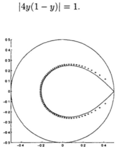
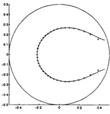
= 1/2, p = 3 1 : 60.Our next bound is more tricky and the underlying idea is borrowed from Szeg5 [71, 1924]. Theorem 2 The zeros Y of Bp(y) satisfy 14Y(1 - Y)I > 21/P.
Here again we see the quadratic polynomial 4Y(1 - Y) appear (see also the preceding subsection). This time, we give a direct analytic proof.
Proof of Theorem 2 . Bp(y) is the truncated Taylor series at y = 0 for (1- y)-P. The pth derivative of this function is p(p + 1) ... (2p - 1)(1 - y)- 2p. Then Taylor's integral formula for the remainder
R,(y) = (1 - y)-P - Bp(y) is
R(y) = (2p - 1) 2(p - 1) Y(y - s)P-1 (1 - s)- 2p ds
(2 ( - 1) fo
= (2p - 1) 2(- 1) ( - t) - (1- yt) - 2 dt
Call this last integral Ip(y). Since each zero has [Yj < 1/2, for any t E (0, 1], |1-Ytj-1 < (1-t/2)- 1 Hence
Ir,(Y)I < (1 - t) - 1 (1 - t/2)-2p
dt
= Ip(1/2).At y = 1/2, Eq.(2.3) gives Bp(1/2) = 2P - 1. Thus the remainder is
R,(1/2) = (1 - 1/2)- 2P-1 = 2P
-At each zero of Bp(y), R,(Y) = (1 - Y)-P. The above equations combine into
14Y(1 - Y)I-P = 4-P Y-P R(Y)I < 14- P(1/2)-P Rp(1/2)I = 1/2.
This is the bound 14Y(1 - Y) proof. (Also see Figure 2-4.)
> 21/P that puts Y outside the limiting curve, and completes the O
Figure 2-4: All zeros lie outside the curve 14y(1 - y)I = 21/p, p = 40.
This idea of using the integral remainder belongs to Szeg6. In [71, 1924], he studied the asymp-totic zero distribution pattern of the partial sum (polynomial) sequence qn(z), obtained from the
Asymptotics of Daubechies Filters and Wavelets
infinite series expansion of ez:
Z2 Zn
qn(z)=1 + z + + .
2! n!
Recent extension of this work can be found in Varga [75, 1992].
2.1.5
Regular Zeros and Singular Zeros
Further analysis exhibits that the zeros of Bp(y) should be better grouped into two sets: those away from y = 1/2 and those near y = 1/2. For convenience, we call them the "regular" zeros and the
"singular" zeros. Regular Zeros
Lemma 3 Fix a 5 > 0. Then uniformly for all ]Yl < 1/2 and ly - 1/21 > 3,
1
I(y) = p( 2) + O(p-2).
Proof. In the integral Ip(y), change variables from t to w = (1 - t)/(1 - yt)2. Then w goes from 1 to 0 and the derivative is dw/dt = (2y - yt - 1)/(1 - yt)3. We leave part of the integral in terms of t
oy 1 - yt
Ip(y) -- -wP-l( 2 yIt)dw.
As p -+ oo the power wP- ' is concentrated near w = 1. Around that endpoint the leading term of the expression in parentheses is (2y - 1)- 1. The integration of wp - 1 gives 1/p and completes the
proof. O
If Y is a zero of B,(y), then R,(Y) = (1 - Y)-P. Therefore
[4Y(1 - Y)]-P 4-P( 2p - 1)2p 2)Ip(Y)
4P2p- 2) (1 + O(p-1)) (2.8)
p - 1 1 -2Y
( - 2Y) (1 + O(p)).
(1 - 2Y)V'4)i
We have applied Eq.(2.6) in the last step. The pth root displays the equation of the approximate curve C, and the error term
Theorem 3 Let 6 > 0 be any fixed small positive number. Then all zeros outside the circle ly -1/21 = 6 are not farther than Ap- 2 from the curve Cp:
14y(1 - y) = I1 - 2yl1/ P (4)/p)
The constant A only depends on 6.
Proof. Let y be the point on Cp nearest to Y Since
I1
+ e1/p = 1 + O(~el/p), we have1- 2YI1/ p = 11 - 2yI / = 1 - 2yl' /. (1
4Y(1- Y)I = 14y(1 - y)l.
= 4y(1 - y)l - 1
and e = Y - y. We must show that e is O(p-2).
S 1/p + 1 - 2y
+o(lE6/p))
1 - 2y O + - y + O(e2) + Ee + O(e2)Iwhere E = (1 - 2y)/(y(1 - y)). E = 0(1) since 6 is fixed. Division yields
14Y(1 - Y)I I1 + Ec + 0(E2)1
=
=
|1
+
EE
+
o(|El)1.
1 - 2YI1/P(4-,rp)1/2 1 + O(+ l Ep)
On the other hand, by Eq.(2.9), the right hand side of the last equation is 1 + O(p-2). Therefore
the left hand side implies that E must be of order O(p-2). D
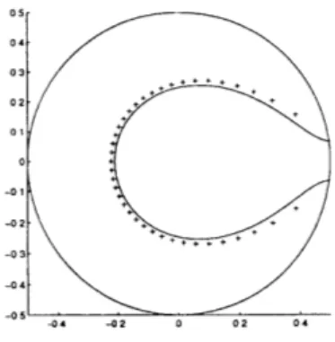
Corollary 1 All zeros outside the circle ly - 1/21 = 6 are not farther than Bp- 1 from the curve D
drawn in Figure 2-5:
14y(1 - y)I = 1 + r,, where p - ln(47rp)2p
P-2p
Here B is a constant only dependent on 6.
A further argument directly based on Eq.(2.8) provides a more detailed information about these regular zeros, which is given in our next theorem:
Asymptotics of Daubechies Filters and Wavelets 05 -04 03 02 -0 1 -03--04
Figure 2-5: DP is a first order approximation curve for regular zeros. p = 40.
fixed (as compared to p) small positive number a,
Uk =rp exp(27ri-), pa< k < p(1-a), kEN,
p
1+ -Uk
Yk = 2 (take the negative real part branch of /)
gives a first order approximation (i.e. with error of order O(p- 1)) to the regular zeros lying outside a circle ly - 1/21 = J(a) for some 6(ca) > 0 and 6(a) -4 0 as a -+ 0.
Please note that the theorem says that on the u-plane, the regular zeros are asymptotically equidistributed.
Singular Zeros
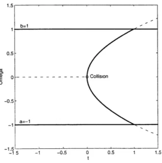
The value of y = 1/2 is in every respect a singular point for this problem. It corresponds to points z = i and z = -i on the unit circle. We now prove that the zeros Y approach 1/2 at speed p-1/2, as Moler discovered by Matlab experiment. Surprisingly, the coefficient of p-1/2 comes from a zero W of the complementary error function
erfc(w) = 1 - erf(w) = e- 2 ds.
The corollary will improve slightly a known result for the location of these zeros.
Theorem 5 If W is a zero of erfc(w), there is a zero Y of Bp(y) and a zero Z of Qp(z) such that
1 W
Y = + + O(p-3/2)
W iW 2
Z = i + O(p-3/2).
Proof. We introduce a new expression for p(y) = (1 - y)PBp(y) (note p(y) = P(z)). As a function of y, this is a polynomial of degree 2p - 1 whose derivative has p - 1 zeros both at y = 0 and y = 1. Therefore the derivative is a multiple of yP-1 (1 - y)p-, and we have an incomplete beta function
p(y) = (1 - y)P Bp(y) = 1 - c 1 22p-1 - t)p 1dt. (2.10)
The number cp is determined by setting y = 1:
"(2p-1 21 p - 2)
cP = 22p-1 t- 1 ( - t)- 1 dt = 22p-1
(p
22-1 (2p - 1)By Stirling's formula, we have
c= (1 + O(p-1)). p
By symmetry, the value of the integral above should be 21- 2pcp/2. Therefore P(1/2) = 1/2. In order
to see the detail of the zeros of Bp(y) near y = 1/2, we introduce a new variable by y - 1/2 = w/2v .
Then p(y) = p(1/2 + w/2v') = p(1/2) - c 1 2 2p-1 (1/2 + t)- 1 (1/2 - t)p-1 dt = 1/2 - 2 c (1 - 4t2)p-1 dt = 1/2 - e-4pt2 dt (1 + O(p-1)) = 1/2- eS2 d (1 + O(p-1)) = 1/2erfc(w) + O(p- 1)
Let W be a zero of erfc(w). All zeros are simple, because the derivative e-"2 is never zero. The fundamental theorem of complex analysis says that as p -+ co, p(1/2 + w/2v/-) is zero at some point
w = W + O(p-'). In terms of y, Y = 1/2 + W/2vi/ + O(p-3/2). This completes the proof since
B,(y) shares every zero with p(y) except y = 1. O
As an interesting application, we can infer certain behaviors of the zeros of the complementary error function.
Corollary 2 Every zero of erfc(w) has I arg W1 < 37r/4.
Asymptotics of Daubechies Filters and Wavelets
at y = 1/2 with slopes ±1. In the limit, W = (Y - 1/2)/f + O(p- 1) must have
I
arg WI _ 37r/4.If the equality held, W2 would be purely imaginary. Then the previous theorem would give
14Y(1 - Y)I =
I1
- W2p- 1 + O(p-2)j = 1 + O(p-2)This contradicts the inequality 14Y(1 - Y)j > 21/p in Theorem 2, proving the corollary. O Fettis, Caslin, and Cramer [26, 1973] computed the zeros of erfc(w) to very high accuracy. They also proved an asymptotic form of the statement
I
arg W15
37r/4. It is interesting to see the complete statement (which their numerical table confirms) proved by such an indirect argument involving the zeros of Bp(y).These zeros approach 1/2 at order p-1/2, close to the line Y
-1/2 = W/2V/ . By the corollary, the slope of this line is not ±1. Therefore the distance from Y to the limiting curve C is of strict order p-1/2 near y = 1/2. In this region, the error order in Eq.(2.9) rises to p-1. This applies in particular to the rightmost zero, which comes from the first W tabulated in [26, 1973], Y - 1/2 + (-1.3548... + il.9914... )/2/p-.
2.1.6
Transition Bandwidth
It is no surprise to see the connection to the error function. Probability theory has already made the error function a universal cumulative distribution function through the Central Limit Theorem. In analysis, the error-function-like behavior is universally shared by certain integrals with a large parameter. In this subsection, we apply this idea to find the transition bandwith of the Daubechies product filter P(e W), a quantity very important in signal processing.
A change of variables t = (1 - cos 8)/2 in Eq.(2.10) produces the integral of sin2p- 1
0. The limits of integration are related by y = (1 - cos0)/2. Thus Eq.(2.10) leads to the Meyer's form [50, 1992] of the halfband filter P(z) in Eq.(2.2):
P(e") = 1- cp1 sin2p- 1 d. (2.11)
The zero at y = 1 becomes the celebrated "zero at 7r" for the frequency response P(eiw). This zero at w = r is of order 2p, from the power of sin 9 in the above integral and the form of P(z) in Eq.(2.2). Factorization gives pth order zeros for the Daubechies polynomials in P(z) = H(z)H(z-1).
That zero at w = 7r and z = -1 is responsible for the p vanishing moments in the wavelets.
The trigonometric polynomial P(e'w) drops monotonically from one to zero on 0 < w 7r. The first 2p - 1 derivatives are zero at w = 0, and w = 7r, from the vanishing of sin2p- 10. Furthermore,
this integral of (1 - cos
0)P-'
sin 0 involves only odd powers of cos 0, and the only even power is the constant term. P(e") is odd around its value 1/2 at w ' = 7r/2, and it is called "halfband".An important question for such a filter is the slope at w = r/2. This slope determines the width of the frequency band, in which P drops from 1 to 0. An ideal filter has a jump; its graph is a brick wall (however, this ideal is not a polynomial). An optimally designed polynomial of order N has slope nearly O(N- 1). There will be ripples in the graph of P(e'w)-a monotonic polynomial
cannot provide such a sharp cutoff. The Daubechies filters are necessarily less sharp: O(N) becomes
O(VN).
Theorem 6 The slope of P(e") is approximately V/-p/r at w = 7r/2. The transition from nearly 1 to nearly 0 is over an interval (i.e. transition band ) of with 2 2/p.
Proof. The integral in Eq.(2.11) has derivative sin2p- 1(7r/2) = 1 at w = r/2. The slope of P(e'")
is exactly the constant -c-'. From the proof of the previous theorem, this is - p--/ + 0(p-3/2).
To measure the drop in P(e"w) around w = 7/2, we integrate from 7/2 - /v.,/- to 7r/2 + a//-i.
Shifting by r/2 to center the integral, and scaling by 0 = -/<r , the drop is
/@ 1 ( 7)2p-d
cP' sin2p - 1 dO 0--
2p-J0 / V/- Cp vF 2p
1/
- - er2 dT.
Thus 95% of the drop comes for a = v/ (within two standard derivatives of the mean, for the normal distribution). This transition interval has width AAw = 2 -2p, as the theorem predicts. That rule was found experimentally by Kaiser and Reed at the beginning of the triumph of digital filters. O
2.2
Asymptotics of Daubechies Mini-phase Wavelets
2.2.1
Introduction
Orthogonal wavelets with compact support were announced by Ingrid Daubechies in 1988. For each
p = 1, 2, - --, she created a wavelet supported on [0, 2p - 1] with p vanishing moments. Our goal is to understand the asymptotic behavior of the scaling functions and the wavelets as p -+ oc. The construction begins with the "maxflat minphase lowpass filter" of length 2p. From its coefficients
hp[n] we form the transfer function or the filter polynomial Hp(z), and there are four main steps to analyze as p -+ oc:
Asymptotics of Daubechies Filters and Wavelets
(2) The phase of Hp(z) on the unit circle z = eiw(we keep using Hp(w) for Hp(eiw)), (3) The scaling function Op(t) with Fourier transform
I-=,l Hp(w/2k),
(4) The wavelet wp(t) = k(-1l)nhp[2p - 1 - n]¢p(2t - n).
In the previous section, we have analyzed the zero distribution of Hp(z). The phase analysis of
H,(z) was carried out in Kateb and Lemari6 [41, 1995]. This section brings step (3) and (4) near to
completion, based on the Kateb-Lemari6's analysis of step (2). The phase is of crucial importance because orthogonal filters cannot be symmetric (beyond the Haar case p = 1). We show that the filter coefficients and the scaling functions have similar asymptotic behavior (but not identical! See
Section 6).
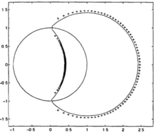
The zeros of H7o(z) are shown in Figure 2-6. There are 70 zeros at z = -1, or w = 7r, which makes the function "maxflat". The other 69 zeros are inside the unit circle, which makes it "miniphase". The graph of IH70(w) shows that the filter is "lowpass"; the magnitude is near zero for high
fre-quencies. This graph approaches the ideal one-zero function as p -+ 00. Then the magnitude of the infinite product p(w) = k0=1 Hp(w/2k) approaches the characteristic function of [-7r, 7r].
15+ + + +++++++ 05 0 -05 -1 ++ +++ +++ -15 ++++ -1 -05 0 05 1 15 2 25
Figure 2-6: H70 has 70 zeros at z = -1 (not shown in the graph) and 69 zeros inside
the unit circle. Those outside the unit circle in the graph are their reciprocals. The z-transform (z+z -1/2 = 1-2y) of the limit curve 14y(1-y)l = 1 in y-plane is two intersected circles Iz ± 11 = v'2 in z-plane. By Theorem 1, all preimages of Y's are in the right half plane: half inside the unit circle and half outside. We take all the zeros inside to construct the Daubechies mini-phase filter Hp(z) according to Eq.(2.5). Those zeros approach the circular arc Iz + 11 = Vr2 from inside by Theorem 2 (see also Figure 2-6).
From the two asymptotic formulas for the zeros (along the circular arc and near the end points
linear factors and added phases. The result is naturally expressed in terms of the group delay grd: grd(Hp(w)) = - (phase of Hp(w)) = pg(w) + O(pl/2 ), (2.12) with 1 1 cos 1 - sinw g(w) = + In (2.13) 2 27r sin w 1 + sin w
(The 1/2 term was not in Kateb and Lemari6's paper [41, 1995] and appears here because we shifted the highpass filter to make it causal.) This even function g(w) is analytic and convex on (-r, 7r). Its
Taylor expansion around w = 0 is (1/2 - 1/r) + w2/6r + O(w4). Its derivative is infinite at w = ±7r.
Our step (3) in the analysis must work with the infinite product p(w) = fI ,= Hp(w/2k). The
phases add, and the derivative for the group delay contributes a factor 1/2k. This makes the infinite
sum converge: grd(¢p(w)) = pG(w) + O(pl/2 ) (2.14) with G() = 2 2 )(2.15) k=1
The function G(w) and its derivative are shown in Figure 2-7. The series for G(w) gives G(0) = g(0) = 1/2 - 1/r and G"(0) = g"(0)/7 = 1/217. The numbers To = G(0) 2 .1817 and 7r = G(ir) .3515 will be called the transition time in the eventual asymptotic formula for p,(7), with r = t/p.
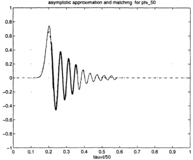
We note an important difference in the time scale t/p, compared to the asymptotics of B-splines (see Unser, Aldroubi and Eden [46, 1992]). The splines are symmetric. They approach Gaussians with scaling tl, . The spline wavelets approach cosine-modulated Gaussians on that scale too. The Central Limit Theorem is at work. Our problem requires a further step, and the technical tool will be the method of stationary phase. This enters when we invert the Fourier transform:
P p(t(w)e t 1 e-ipG(-')(w)ettw dw = ]p(t). (2.16)
The scaled phase is approximately G(-1) (w) =
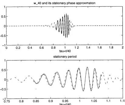
![Figure 2-11: Plot of - log 0 Ih,[n] I with p = 100, 0 < n < 2p - 1 = 199](https://thumb-eu.123doks.com/thumbv2/123doknet/14116862.467074/50.918.250.696.172.444/figure-plot-log-ih-n-i-lt-lt.webp)
