Investigation of hydro-acoustic tracking capability using multiple collaborating ocean gliders

(1)

Publisher’s version / Version de l'éditeur:

Vous avez des questions? Nous pouvons vous aider. Pour communiquer directement avec un auteur, consultez la Questions? Contact the NRC Publications Archive team at

PublicationsArchive-ArchivesPublications@nrc-cnrc.gc.ca. If you wish to email the authors directly, please see the first page of the publication for their contact information.

https://publications-cnrc.canada.ca/fra/droits

L’accès à ce site Web et l’utilisation de son contenu sont assujettis aux conditions présentées dans le site LISEZ CES CONDITIONS ATTENTIVEMENT AVANT D’UTILISER CE SITE WEB.

Student Report; no. SR-2010-20, 2010-12-20

READ THESE TERMS AND CONDITIONS CAREFULLY BEFORE USING THIS WEBSITE.

https://nrc-publications.canada.ca/eng/copyright

NRC Publications Archive Record / Notice des Archives des publications du CNRC : https://nrc-publications.canada.ca/eng/view/object/?id=8f6d88ab-11fd-4db3-bacf-cf25d23d09e1 https://publications-cnrc.canada.ca/fra/voir/objet/?id=8f6d88ab-11fd-4db3-bacf-cf25d23d09e1

NRC Publications Archive

Archives des publications du CNRC

For the publisher’s version, please access the DOI link below./ Pour consulter la version de l’éditeur, utilisez le lien DOI ci-dessous.

https://doi.org/10.4224/17712926

Access and use of this website and the material on it are subject to the Terms and Conditions set forth at

Investigation of hydro-acoustic tracking capability using multiple

collaborating ocean gliders

(2)

DOCUMENTATION PAGE

REPORT NUMBER

SR-2010-20

NRC REPORT NUMBER DATE

December 2010

REPORT SECURITY CLASSIFICATION

Unclassified

DISTRIBUTION

Unlimited

TITLE

INVESTIGATION OF HYDRO-ACOUSTIC TRACKING CAPABILITY USING MULTIPLE COLLABORATING OCEAN GLIDERS

AUTHOR (S)

Kasun Somaratne

CORPORATE AUTHOR (S)/PERFORMING AGENCY (S)

National Research Council, Institute for Ocean Technology, St. John’s, NL

PUBLICATION

SPONSORING AGENCY(S)

IOT PROJECT NUMBER NRC FILE NUMBER

KEY WORDS

Tracking system, sound source, hydrophones, arrays

PAGES iii, 29, App. A-E FIGS. 19 TABLES 1 SUMMARY

The possibility of a hydro-acoustic tracking system was investigated by developing a theoretical model using the underlying principles of sound propagation through water. The effectiveness of the tracking system depends on its ability to determine the direction and range to a sound source using multiple arrays of sound detectors (hydrophones). In three dimensional space it was found that at least four hydrophones are needed to determine the direction vector to a sound source. To determine the range to a sound source at least two physically separated arrays of at least four hydrophones are needed.

To obtain an accurate direction vector to the sound source the relative time delay between the hydrophones in an array must be accurately determined. Cross-correlation of two audio signals provide the relative time shift, where the accuracy is primarily limited by the

sampling frequency.

A procedure was developed to accurately detect the direction and range to a sound source using audio and position data from the hydrophones. A preliminary experiment was

performed in air using microphones to test the performance of the developed sound source detection system in two dimensions. The results from the initial experiment were

unsuccessful due to the smaller baseline between the microphones. It was found that larger baselines provide more accurate results.

More testing should be conducted to quantify the performance of the developed sound source detection method. This method should be tested against different sound sources, different environments and different geometrical arrangements to identify its limitations. Finally, the hydrophone arrays will be integrated into ocean gliders and tested at sea

ADDRESS National Research Council

(3)

National Research Council Conseil national de recherches Canada Canada Institute for Ocean Institut des technologies Technology océaniques

INVESTIGATION OF HYDRO-ACOUSTIC TRACKING CAPABILITY

USING MULTIPLE COLLABORATING OCEAN GLIDERS

SR-2010-20

Kasun Somaratne

(4)

Summary

The possibility of a hydro-acoustic tracking system was investigated by developing a the-oretical model using the underlying principles of sound propagation through water. The effectiveness of the tracking system depends on its ability to determine the direction and range to a sound source using multiple arrays of sound detectors (hydrophones). In three dimensional space it was found that at least four hydrophones are needed to determine the direction vector to a sound source. To determine the range to a sound source at least two physically separated arrays of at least four hydrophones are needed.

To obtain an accurate direction vector to the sound source the relative time delay between the hydrophones in an array must be accurately determined. Cross-correlation of two audio signals provide the relative time shift, where the accuracy is primarily limited by the sampling frequency.

A procedure was developed to accurately detect the direction and range to a sound source using audio and position data from the hydrophones. A preliminary experiment was performed in air using microphones to test the performance of the developed sound source detection system in two dimension. The results from the initial experiment was unsuccessful due to the smaller baseline between the microphones. It was found that larger baselines provide more accurate results.

More testing should be conducted to quantify the performance of the developed sound source detection method. This method should be tested against different sound sources, different environments and different geometrical arrangements to identify its limitations. Finally, the hydrophone arrays will be integrated into ocean gliders and tested at sea.

(5)

List of Figures

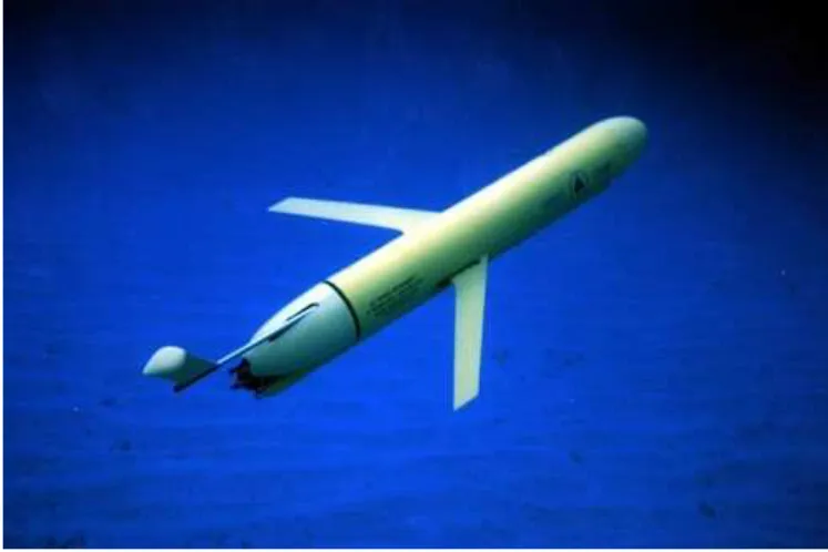
1 Image of an ocean glider. . . 1 2 The direction of a sound source is ambiguous if only three hydrophones are

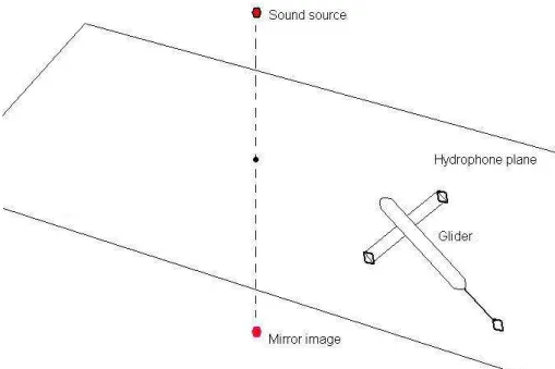
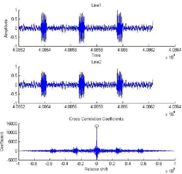
used in three dimensional space (can be above or below the plane of the hydrophones). . . 2 3 The cross-correlation sequence of two audio plots. The relative shift at

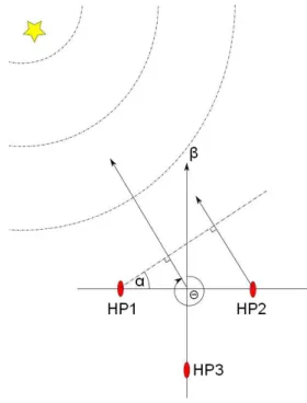
which the correlation coefficient is a maximum is the time delay between the two hydrophones. . . 4 4 Top view of a glider with three hydrophones. . . 5 5 Geometrical parameters for determining the location of the sound source. . 5 6 Coordinate frames for calculating the position of a sound source in 3D. . . 6 7 The experimental setup with a sound source and two microphones. The

objective of the experiment is to find the angle α. . . 9 8 The calculated direction angle as a function of ∆t for baselines of 0.07 m,

0.1 m and 0.15 m, showing low angular resolution for shorter baselines. . . 9 9 Error in source position as a function of error in the measured yaw, pitch

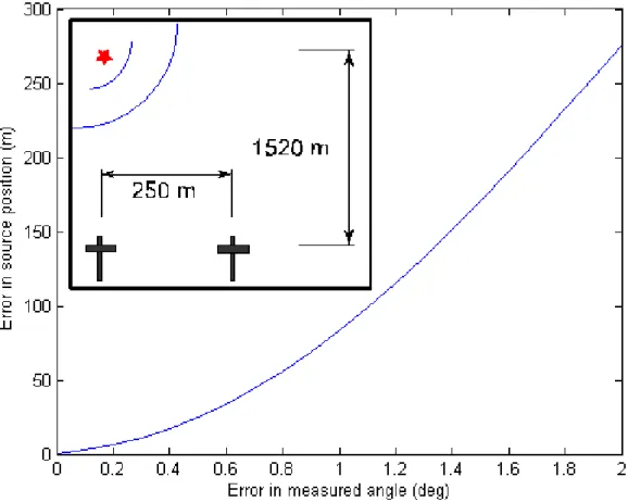
and roll angles of the gliders. The geometrical arrangement of the sound source and the gliders are shown in sub plot. . . 10 10 Error in source position as a function of error in the measured yaw, pitch

and roll angles of the gliders. The geometrical arrangement of the sound source and the gliders are shown in sub plot. . . 12 11 A glider with three hydrophones. Two hydrophones are fixed to the payload

module. . . 24 12 A glider with three hydrophones. Two hydrophones are fixed to the wings. 25 13 Glider wing design with embedded hydrophone cable. . . 26 14 Hydrophone mount and safety cap. . . 27 15 An ocean glider that will be used to deploy the hydrophones. . . 28 16 A payload bay where all the electronic equipment used for sound source

detection will be mounted. . . 28 17 Marantz Professional PMD661 sound recorder used to record audio data

from the hydrophones. . . 29 18 B&K 2634 charge amplifier used to amplify the audio signal from the

hy-drophones. . . 29 19 B&K Type 8103 hydrophone . . . 29

List of Tables

1 Comparison of measured direction angle to the calculated direction angle of a sound source in two dimensional space. . . 11

(7)

1 Introduction

In a liquid medium (i.e. water), where communications through radio waves fall short, sound waves provide a possible mechanism to transfer information. The ability to detect the direction and range to discreet sound sources has applications from guiding underwater vehicles to surveillance activities. Sound can also be used to study marine life.

Figure 1: Image of an ocean glider.

As sound propagates through a medium it is subjected to various forms of absorption, scattering and reflection which makes it rather a poor carrier of information in compar-ison with the electromagnetic waves in air. However, in a dense medium such as water electromagnetic waves fail to penetrate deep enough to be able to carry information to larger distances. Therefore, sound is believed to be the only practical way to propagate signals to greater distances at sea (Jensen 1994). Furthermore, a good understanding of the acoustic environment (i.e. the ocean) helps us overcome the difficulties imposed by the scattering and absorption properties of sound in water.

One other property that differs sound waves from electromagnetic waves is the speed of propagation. The velocity of electromagnetic waves is a constant1

, in contrary the sound speed changes depending on the properties of the medium. The sound speed in water is affected by the water temperature, salinity and pressure (Etter 2003). As a result sound does not always take the most direct path from the sound source to the detector. Depending on how far the sound source is (or its intensity) it may be audible only through specific sound channels.

As a result of low transmission losses in underwater sound channels small explosive sound sources are even heard half way across the globe (Jensen 1994). In such case where the sound is propagated through a specific sound channel rather than the direct route it may seem to the detector as if the sound is coming from a different direction. Therefore,

(8)

it is important to have an idea of the existing sound channels as a result of the gradients in temperature, salinity and pressure.

The purpose of this report is to present a theoretical model, which allows the deter-mination of the direction and the range to a discrete sound source as observed by two or more ocean gliders containing multiple detectors (hydrophones), and to report on the tests conducted to validate the theory.

2 Materials and Methods

In one dimension, at least two omnidirectional hydrophones are needed to determine the direction of a sound source. In this case the direction is easily obtained by determining which hydrophone received the signal first. In two dimensions at least three hydrophones, not arranged in a line, are needed to determine the direction of a sound source.

Figure 2 shows the ambiguity in direction caused by using only three hydrophones to determine source direction in three dimensional space (3D). To eliminate this ambiguity at least four hydrophones, not in a plane, are required.

Figure 2: The direction of a sound source is ambiguous if only three hydrophones are used in three dimensional space (can be above or below the plane of the hydrophones).

The position of the sound source can be obtained by triangulating two directional vectors to the sound source. In order to calculate the source position two sets of information are needed: The positions of the hydrophones and the time delay between signal arrival

(9)

times at each hydrophone. The positions of the hydrophones can be obtained if the glider position and the orientation are known.

The time delay between the hydrophones can be easily determined using the audio data of the hydrophones. The audio data of the hydrophones are stored in 96 kHz 24-bit PCM format. A method of cross-correlation is used to identify the time delay between the hydrophones. The cross-correlation coefficient, defined in Equation 1, characterizes the similarity between two signals, x(n) and y(n).

Rxy(m) = lim N →∞ 1 N N −1 ∑ n=0 x(n)y(n + m) − ∞ < m < ∞ (1) A plot of the cross-correlation coefficients of two audio signals are shown in Figure 3. The time delay between the plots in Figure 3 is the relative shift at which the correlation coefficient is a maximum (i.e. when the two functions nearly overlap with each other).

3 Determining the direction of a sound source in the

same plane as the hydrophones of a glider

A special case of finding the sound source direction occurs when the sound source is restricted to the plane formed by three hydrophones. This problem can be easily solved if three assumptions are made. The first assumption is that the sound source is far away in comparison to the baseline formed by the hydrophones. Secondly, the speed of sound in water is assumed to be a constant. The third assumption is that the sound takes the most direct path to the hydrophones. Sound is subjected to refraction, absorption and reflection as it travels through the water. The second and the third assumption might not necessarily be true. However, to correct for such effects a greater understanding of the ocean environment is needed.

Figures 4 and 5 show the geometrical setting for the calculation of source direction (θ) given the glider heading (β), the time delay between HP1 and HP2 (∆t12) and the time delay between HP1 and HP3 (∆t13). The angle α can be easily calculated using the right angled triangle in Figure 5 as shown in Equation 2.

α= sin−1(|∆t12| × c w

)

(2) The sign of ∆t13 helps determine whether the sound source is located ahead of the glider or behind the glider. Using this information along with the heading of the glider, the direction of the sound source (θ) can be determined as shown in Equation 3.

θ =        180◦ + α + β ∆t13 ≥ 0 and ∆t12 ≤ 0 180◦ − α + β ∆t13 ≥ 0 and ∆t12 >0 360◦ − α + β ∆t13 < 0 and ∆t12 ≤ 0 α+ β ∆t13 < 0 and ∆t12 >0     (3)

(10)

Figure 3: The cross-correlation sequence of two audio plots. The relative shift at which the correlation coefficient is a maximum is the time delay between the two hydrophones.

(11)

Figure 4: Top view of a glider with three hydrophones.

(12)

4 Determining the position of a sound source in 3D

space

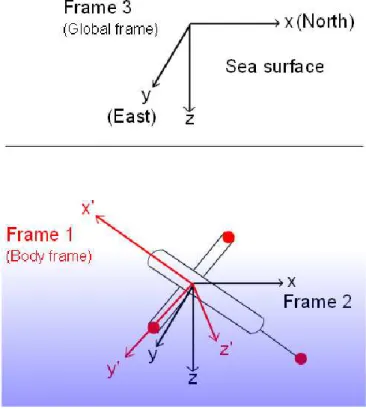
To determine the position of a sound source in 3D space at least two gliders each with four hydrophones are needed. The position is determined by first obtaining a direction vector to the sound source from each glider, and then by using the method of triangulation. In order to find the position of a sound source a coordinate system(s) has to be defined. Figure 6 shows three reference frames defined using one of the gliders.

To obtain a direction vector to the sound source, first select a glider and determine the hydrophone which received the signal first. Assume the time it took for the sound to reach the first hydrophone is one second. Then the time it took for the signal to reach the other two hydrophones can be calculated using their relative time differences. For each hydrophone there is a spherical shell, centered at the position of the hydrophone, where the sound source could be possibly located. The radius of such a sphere can be calculated using the constant sound speed and the time it took for the signal to reach the hydrophone. Once such a sphere is determined for each hydrophone of a glider the solution simplifies down to finding the intersection point of the spheres (Equations 4,5,6,7).

(13)

(x − x1) 2 + (y − y1) 2 + (z − z1) 2 = r2 1 (4) (x − x2) 2 + (y − y2) 2 + (z − z2) 2 = r2 2 (5) (x − x3) 2 + (y − y3) 2 + (z − z3) 2 = r2 3 (6) (x − x4) 2 + (y − y4) 2 + (z − z4) 2 = r2 4 (7)

The mathematical solution of finding the intersection point of the four spheres is ex-plained in greater detail in appendix A. Assume the calculated intersection point (i.e. di-rection vector) in Frame 1 is ⃗R1. The same procedure as described above can be followed with the second glider to obtain another direction vector ( ⃗R2). However, the positions of the hydrophones of the second glider must be transformed into Frame 1 before finding the direction vector. Rx(γ) =   1 0 0 0 cos(γ) −sin(γ) 0 sin(γ) cos(γ)   Ry(β) =   cos(β) 0 sin(β) 0 1 0 −sin(β) 0 cos(β)   Rz(α) =   cos(α) −sin(α) 0 sin(α) cos(α) 0 0 0 1   R= Rx(γ)Ry(β)Rz(α) (8) γ = γ1− γ2 β = β1− β2 α = α1− α2

Each of the rotation matrices, Rx(γ), Ry(β) and Rz(α) corresponds to the rotations in yaw, pitch and roll between the two gliders respectively. The full rotation between the two gliders is accounted for by the rotation matrix R as shown in Equation 8. The transformation of the hydrophone coordinates to Frame 1 (⃗p → ⃗p′_{) is done by multiplying} with a rotation matrix and applying a linear transformation (⃗s) as shown in Equation 9. ⃗s is the position vector of the second glider in Frame 1.

⃗ p′

= R × ⃗p + ⃗s (9)

Two lines (rays) can be defined using the two direction vectors and the positions of the gliders. The position of the sound source can be calculated by finding the intersection between these two lines. However, due to measurement uncertainties the two lines may be

(14)

skewed and may not necessarily intersect. In such case the two points in each line where the shortest distance between them occur must be calculated. This provides a region in 3D for the possible location of the sound source. The mathematical details of finding the shortest distance between two lines is explained in Appendix B.

Finally, after obtaining the source position in Frame 1 it can be easily transformed to the global frame.

5 Experiments

Several experiments were performed to test the theory presented in the previous section. The experiments were performed in air using microphones instead of hydrophones in water. The physics of sound travel in air and water is similar and therefore the above theory is valid in both cases. It is more convenient to perform simple experiments in air than in water.

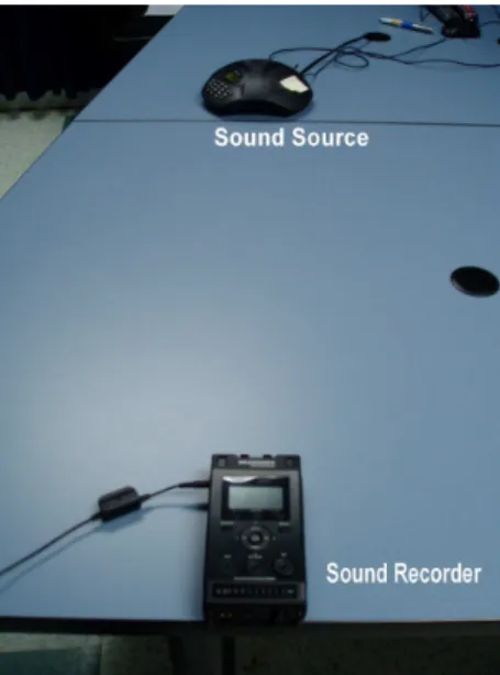
The experimental setup is shown in Figure 7. The objective of the experiment is to correctly determine the direction of the sound source using the audio data from the two built-in microphones of the sound recorder.

The experiment was carried out in a closed room. A telephone is used as a sound source, which has three speakers. A Marantz Professional PMD661 stereo sound recorder was used for this experiment. The separation between the microphones is seven centimetres. The sampling frequency of the audio is 96 kHz, which amounts to a time resolution of 0.000010416 s. Using a sound speed in air of 340.29 ms−1

the minimum separation between the microphones required to resolve a sound source is 3.5 mm. The angular resolution at 96 kHz sample frequency and a 0.07 m baseline is ∼ 3◦

.

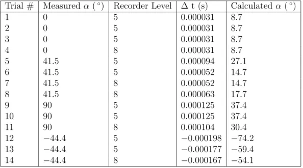
Table 1 lists the results of the experiment. Multiple audio samples were taken with the same settings to test consistency of the results. The time delay between the two audio signals, ∆t, is obtained by cross correlation of the two signals. The angle α is defined as in Figure 7 and is calculated by a software implementation of the method described in the previous section.

The results do not quite agree with the measured values of α. Also the results vary by as much as 20◦

in some occasions. The main cause of this is the low angular resolution inflicted by the smaller baseline. Figure 8 shows how rapidly the direction angle changes as a function of ∆t for different baselines. The plot rises less steeply for longer baselines, which gives a higher angular resolution.

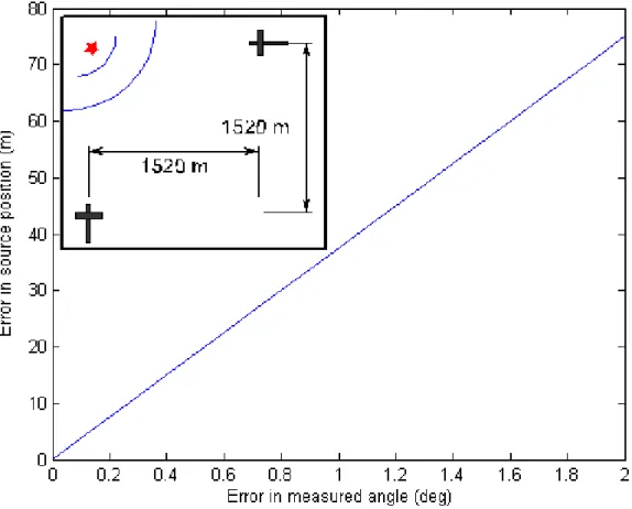
A computer simulation was carried out to estimate the error in calculated source po-sition arising from measurement errors of the orientation of the gliders. Two gliders with four hydrophones each were used for the simulation as shown in Figure 9. The simulation attempts to calculate the position of a sound source (position already known) using the position of the gliders, the orientation of the gliders and the signal arrival time at each hydrophone. An error value was added to the yaw, pitch and the roll of each glider and the difference between the calculated source position and the actual source position was

(15)

Figure 7: The experimental setup with a sound source and two microphones. The objective of the experiment is to find the angle α.

Figure 8: The calculated direction angle as a function of ∆t for baselines of 0.07 m, 0.1 m and 0.15 m, showing low angular resolution for shorter baselines.

(16)

Figure 9: Error in source position as a function of error in the measured yaw, pitch and roll angles of the gliders. The geometrical arrangement of the sound source and the gliders are shown in sub plot.

(17)

Table 1: Comparison of measured direction angle to the calculated direction angle of a sound source in two dimensional space.

Trial # Measured α (◦

) Recorder Level ∆ t (s) Calculated α (◦ ) 1 0 5 0.000031 8.7 2 0 5 0.000031 8.7 3 0 5 0.000031 8.7 4 0 8 0.000031 8.7 5 41.5 5 0.000094 27.1 6 41.5 5 0.000052 14.7 7 41.5 8 0.000052 14.7 8 41.5 8 0.000063 17.7 9 90 5 0.000125 37.4 10 90 5 0.000125 37.4 11 90 8 0.000104 30.4 12 −44.4 5 −0.000198 −74.2 13 −44.4 5 −0.000177 −59.4 14 −44.4 8 −0.000167 −54.1 obtained.

A plot of the source position error as a function of the error in the measured yaw, pitch and roll angles is shown in Figure 9. It should be noted that these results are specific to the geometrical arrangement used for the simulation. other arrangements of the gliders and the sound source was found to give different error estimates. Figure 10 shows a different arrangement of the gliders providing larger error estimates than in Figure 10 for the same position of the sound source. Thus certain arrangements of the hydrophone arrays provide better detection accuracy for certain regions.

This model must be tested with baselines similar to the ones that will be used on the gliders before evaluating its suitability for the proposed tracking system. However, at the time of writing of this report the equipment necessary to do such an experiment was not available.

(18)

Figure 10: Error in source position as a function of error in the measured yaw, pitch and roll angles of the gliders. The geometrical arrangement of the sound source and the gliders are shown in sub plot.

(19)

6 Conclusion

A concept and theory was developed to investigate the possibility of an underwater acoustic tracking system. It was found that at least four hydrophones not arranged in a plane are needed to determine the direction to a sound source in 3D space. The possible location of a sound source can be calculated by the method of triangulation using at least two sets of four hydrophones.

The time delay between the signal arrival times at each hydrophone can be obtained by cross-correlation of the audio data from each hydrophone. A simple experiment was performed in air to test the performance of the sound source detection method. The smaller baseline used for this initial experiment failed to provide accurate values for the direction of the sound source. Longer baselines provide more accurate results. Certain arrangements of the hydrophone arrays provide better detection accuracy for certain regions.

7 Future Work

More testing should be done to verify the performance of the sound source detection method preferably with longer baselines, different sound sources and different geometrical arrangements of the sound source and the sound detectors. Once it has been proven to work in air it must be tested in water using hydrophones, which will be used on the gliders. The hydrophones and the necessary electronic components should then be attached to the gliders and tested to see if the baselines are adequate for correctly determining the source direction. Finally multiple gliders with hydrophones should be tested in an ocean environment to see their effectiveness in detecting and tracking discrete sound sources.

Acknowledgments

I would like to thank my supervisor Mr. David Millan and Dr. Christopher Williams for their help with the project.

(20)

Bibliography

Dufaux, A., “Detection and Recognition of Impulsive Sound Signals”, 2001, Institute of Microtechnology, University of Neuchatel, Switzerland

Etter, P.C., “Underwater Acoustic Modeling and Simulation”, 3rd _{edition, 2003, Spon} press, London and New York, ISBN 0-419-26220-2

Hobson, A.J., “Vector equations of straight lines”, Just the Maths, 8.5.6, http://nestor2.coventry.ac.uk/jtm/slides/contents.htm

Jensen, F.B., Kuperman, W.A, Porter, M.B., Schmidt, H., “Computational Ocean Acoustics”, 1994, AIP Press, New york, ISBN 1-56396-209-8

Marsh, H.W., Schulkin, M., Kneale, S.G., “Scattering of Underwater Sound by the Sea Surface”, 1961, The journal of the Acoustical Society of America, 33, 3

Petrie, B., Loder, J.W., Akenhead, S., Lazier, J., “Temperature and Salinity Variability on the Eastern Newfoundland Shelf: The Annual Harmonic”, 1989, Atmosphere-Ocean, 29,19

Song, K.T., Chen, J.L., “Sound Direction Recognition Using a Condenser Microphone Array”, 2003, IEEE, International Symposium on Computational Intelligence in Robotics and Automation, 1445

(21)

A

Finding the intersection point of four spheres

Suppose the equations of the four spheres are given as in Equations 10, 11, 12 and 13. Subtract Equation 10 from Equations 11 and 12 to obtain equations 14 and 15 respectively. Equations 14 and 15 are the planes of intersections between the first three spheres.

(x − x1)2 + (y − y1)2 + (z − z1)2 = r2 1 (10) (x − x2) 2 + (y − y2) 2 + (z − z2) 2 = r2 2 (11) (x − x3) 2 + (y − y3) 2 + (z − z3) 2 = r2 3 (12) (x − x4) 2 + (y − y4) 2 + (z − z4) 2 = r2 4 (13) ax+ by + cz = d (14) ex+ f y + gz = h (15) a = 2(x1− x2) b = 2(y1− y2) c = 2(z1− z2) d = r2 2 − r 2 1− x 2 2+ x 2 1− y 2 2+ y 2 1− z 2 2 + z 2 1 e = 2(x1− x3) f = 2(y1− y3) g = 2(z1− z3) h = r2 3 − r 2 1− x 2 3+ x 2 1− y 2 3+ y 2 1− z 2 3 + z 2 1

Then find the parametric equations of the line of intersection between these two planes. ⃗

n1 and ⃗n2 are normal vectors to the two planes.

⃗ n1 =   a b c  n2⃗ =   e f g   M =[ ⃗n1 n2⃗ ]T T =[d h ]

The position vector ( ⃗x0) of the line is given by a particular solution to the equation M x0 = T . The direction vector, ⃗l is given by the cross product of the vectors ⃗n1 and ⃗n2.

⃗ x0 =   k m q  ⃗l =   l n r  

(22)

The parametric equations of the line given by Equations 16, 17 and 18 are then substituted into Equation 10, which gives a quadratic equation of one variable (Equation 19).

x= k + lt (16)

y = m + nt (17)

z = q + rt (18)

At2+ Bt + C = 0 (19)

Equation 19 is solved to find the two roots which are then substituted back into Equa-tions 16, 17 and 18 to find the two possible posiEqua-tions for the sound source. To determine the correct position for the sound source substitute the position coordinates into Equation 13 (Equation of the fourth sphere) and pick the point that lies on the sphere. It is possible that neither of the two roots lie exactly on the sphere due to measurement errors. In such case choose the position which is closest to the surface of the fourth sphere.

⃗ r′ =   r1 r2 r3  

B

Finding the shortest distance between two skewed

lines

Define the two lines, L1 and L2 as in Equation 20 and 21 with the position vectors ⃗s1 and ⃗

s2 and the direction vectors ⃗r1 and ⃗r2.

L1 = ⃗s1+ ⃗r1t (20)

L2 = ⃗s2+ ⃗r2t (21)

Now take the normalized cross product (⃗dl) of the direction vectors of the two lines. Extend the lines L1 and L2 along ⃗dl to form two planes, P1 and P2 respectively.

⃗

dl = ⃗r1× ⃗r2 (22)

P1 = ⃗s1+ ⃗r1u+ ⃗dlv (23) P2 = ⃗s2+ ⃗r2u+ ⃗d2v (24)

(u, v ∈ R)

Calculate the intersection points between P1 and L2 (I1) and between P2 and L1 (I2). These two points are the points of the two lines which gives the shortest distance between them. Finally, take the center position between the two intersection points and take it as the location of the sound source. The intersection points give the uncertainty of the position.

(23)

C

Software Implementation - Matlab code

C.1 Triangulation of a sound source using two arrays of four

hydrophones each

function [spos] = Tri3D v6( Glider1, Glider2, t1, t2, t3, t4, t5, t6, t7, t8 )

% TRI3D V6 This function calculates the position of a sound source using two % arrays of four hydrophones each.

% Glider1, Glider2: 1X7 arrays containing [x;y;z;yaw;pitch;roll;depth] % t1..t4: signal arrival times at Glider1 hydrophones

% t5..t8: signal arrival times at Glider2 hydrophones

gpos1 = Glider1(1:3); yaw1 = -1*Glider1(4)*pi/180.0; pitch1 = -1*Glider1(5)*pi/180.0; roll1 = -1*Glider1(6)*pi/180.0; depth1 = Glider1(7); gpos2 = Glider2(1:3); yaw2 = -1*Glider2(4)*pi/180.0; pitch2 = -1*Glider2(5)*pi/180.0; roll2 = -1*Glider2(6)*pi/180.0; depth2 = Glider2(7);

% Assumed positions of the Glider1 hydrophones in the Glider1 frame

p1 = [0; -1; 0]; p2 = [0; 1; 0]; p3 = [0; 0; -1]; p4 = [-1; 0; 0];

% The position vectors of hydrophones in Glider2 must be transformed to % the frame of the first glider.

Rx1 = [1, 0, 0;

0, cos(roll1), -1*sin(roll1); 0, sin(roll1), cos(roll1)];

Ry1 = [cos(pitch1), 0, sin(pitch1); 0, 1, 0;

(24)

Rz1 = [cos(yaw1), -1*sin(yaw1), 0; sin(yaw1), cos(yaw1), 0; 0, 0, 1]; R1 = Rx1*Ry1*Rz1; Rx2 = [1, 0, 0; 0, cos(roll2), -1*sin(roll2); 0, sin(roll2), cos(roll2)];

Ry2 = [cos(pitch2), 0, sin(pitch2); 0, 1, 0; -1*sin(pitch2), 0, cos(pitch2)]; Rz2 = [cos(yaw2), -1*sin(yaw2), 0; sin(yaw2), cos(yaw2), 0; 0, 0, 1]; R2 = Rx2*Ry2*Rz2; tp5 = R2’*p1; tp6 = R2’*p2; tp7 = R2’*p3; tp8 = R2’*p4; tp5 = R1*tp5; tp6 = R1*tp6; tp7 = R1*tp7; tp8 = R1*tp8;

ltv = gpos2-gpos1; % in global frame

ltv = R1*ltv;% in body frame of Glider 1

% position coordinates of Glider2 hydrophones in Glider1 frame

p5 = tp5 + ltv; p6 = tp6 + ltv; p7 = tp7 + ltv; p8 = tp8 + ltv;

(25)

[g1dir vec] = getDirvec v2(p1, p2, p3, p4, t1, t2, t3, t4); [g2dir vec] = getDirvec v2(p5, p6, p7, p8, t5, t6, t7, t8); s1 = [0;0;0];

s2 = ltv;

% get the two possible source locations from getPos.m

spos = getPos(s1, s2, g1dir vec, g2dir vec-ltv, depth1, R1);

% print the results:

disp(’possible source location:’)

disp(strcat(’X = ’, num2str(spos(1)), ’ (’, num2str(spos(4)), ’)’)) disp(strcat(’Y = ’, num2str(spos(2)), ’ (’, num2str(spos(5)), ’)’)) disp(strcat(’Z = ’, num2str(spos(3)),’ (’, num2str(spos(6)),’)’))

end

function [ dir vec ] = getDirvec v2( p1, p2, p3, p4, t1, t2, t3, t4)

%getDirvec v2 Calculates the direction vector to a sound source from a glider % p1..p4: The position coordinates of the hydrophones in the form [x;y;z] % t1..t4: The signal arrival time at each respective hydrophone

% Initial setting of variables

Temp = 4.43; Salt = 31.76;

%sound speed = 1449.2 + 4.6*Temp - 0.055*Temp^2 + 0.00029*Temp^3 + (1.34-0.01*Temp)*(Salt-35) + 0.016*depth;

sound speed = 1520.0; epsilon = 1.0;

% Determining which HP received the signal first

t ary = [t1 t2 t3 t4];

[min t, FHP] = min(t ary); FHP = FHP(1);

T1 = t1; T2 = t2; T3 = t3; T4 = t4;

(26)

if (FHP == 1) T2 = 1.0 + T2-T1; T3 = 1.0 + T3-T1; T4 = 1.0 + T4-T1; T1 = 1.0; end if (FHP == 2) T1 = 1.0 + T1-T2; T3 = 1.0 + T3-T2; T4 = 1.0 + T4-T2; T2 = 1.0; end if (FHP == 3) T2 = 1.0 + T2-T3; T1 = 1.0 + T1-T3; T4 = 1.0 + T4-T3; T3 = 1.0; end if (FHP == 4) T1 = 1.0 + T1-T4; T2 = 1.0 + T2-T4; T3 = 1.0 + T3-T4; T4 = 1.0; end

% Calculating radius of the sphere around each HP

r1 = T1*sound speed; r2 = T2*sound speed; r3 = T3*sound speed; r4 = T4*sound speed;

% Planes of intersection between three spheres

a = 2*( p1(1)-p2(1) ); b = 2*( p1(2)-p2(2) ); c = 2*( p1(3)-p2(3) ); d = r2^2-r1^2-p2(1)^2+p1(1)^2-p2(2)^2+p1(2)^2-p2(3)^2+p1(3)^2; e = 2*( p1(1)-p3(1) ); f = 2*( p1(2)-p3(2) ); g = 2*( p1(3)-p3(3) ); h = r3^2-r1^2-p3(1)^2+p1(1)^2-p3(2)^2+p1(2)^2-p3(3)^2+p1(3)^2;

(27)

% line of intersection between the two planes n1 = [a; b; c;]; n2 = [e; f; g;]; M = [n1 n2]’; T = [d; h]; pos vec = M\T;

dir vec = [(b*g-c*f); (c*e-a*g); (a*f-b*e)]; k = pos vec(1); l = dir vec(1); m = pos vec(2); n = dir vec(2); q = pos vec(3); r = dir vec(3);

% calculating the two points of intersection

A = l^2+n^2+r^2; B = 2*k*l-2*l*p1(1)+2*m*n-2*n*p1(2)+2*q*r-2*r*p1(3); C = k^2-2*k*p1(1)+p1(1)^2+m^2-2*m*p1(2)+p1(2)^2+q^2-2*q*p1(3)+p1(3)^2-r1^2; rt1 = real((-B+sqrt(B^2-4*A*C))/(2*A)); rt2 = real((-B-sqrt(B^2-4*A*C))/(2*A)); X1 = k+l*rt1; Y1 = m+n*rt1; Z1 = q+r*rt1; X2 = k+l*rt2; Y2 = m+n*rt2; Z2 = q+r*rt2; sol 1 = (X1 - p4(1))^2 + (Y1 - p4(2))^2 + (Z1 - p4(3))^2; sol 2 = (X2 - p4(1))^2 + (Y2 - p4(2))^2 + (Z2 - p4(3))^2; src x = -99999; src y = -99999; src z = -99999;

if ( sol 1 >= r4^2-epsilon && sol 1 <= r4^2+epsilon ) src x = real(X1);

(28)

src z = real(Z1);

elseif( sol 2 >= r4^2-epsilon && sol 2 <= r4^2+epsilon )

src x = real(X2); src y = real(Y2); src z = real(Z2);

else

error(’Could not find source position :(’)

end

dir vec = [src x; src y; src z];

end

function [ src loc ] = getPos( posvec1, posvec2, dirvec1, dirvec2, depth1, R)

% GETPOS This function triangulates two given direction vectors and finds % the position of the sound source

% posvec1, posvec2: The position vectors of the two gliders

% dirvec1, dirvec2: The direction vectors from each respective glider % depth1: The depth of Glider1 (The main glider)

% R: The rotation matrix associated with the orientation of Glider1. % calculating the intersection between the direction vectors

dl = cross(dirvec1, dirvec2); s1 = posvec1;

s2 = posvec2;

% intersection between line 1 and plane 2

M = [-1*dirvec1, dirvec2, dl]; N = [s1-s2];

param1 = inv(M)*N;

spos1 = s1 + dirvec1*param1(1);

% intersection between line 2 and plane 1

M = [-1*dirvec2, dirvec1, dl]; N = [s2-s1];

(29)

spos2 = s2 + dirvec2*param2(1);

% transforming to global frame

spos1 = [0;0;depth1] + R’*spos1; spos2 = [0;0;depth1] + R’*spos2;

% computing source location

src x = (spos1(1)+spos2(1))/2; src y = (spos1(2)+spos2(2))/2; src z = (spos1(3)+spos2(3))/2; err x = abs((spos1(1)-spos2(1))/2); err y = abs((spos1(2)-spos2(2))/2); err z = abs((spos1(3)-spos2(3))/2);

src loc = [src x, src y, src z, err x, err y, err z];

end

C.2 Estimating error in position of sound source as a result of

errors in measured yaw, pitch and roll angles

function [] = Tri3dtest()

% TRI3DTEST Estimates the error in sound position due to errors in measured % values of yaw, pitch and roll angles

pos = {}; pyaw = {};

for err = 0:0.1:2

Glider1 = [0;0;100;0+err;0-err;0+err;100]; Glider2 = [0;250;100;0-err;0+err;0-err;100];

spos = Tri3D v6(Glider1, Glider2, 1.000000216,1.000000216,1.000000216,1.000657895, 1.013328976,1.013542519,1.013435753,1.014084718);

cpos = sqrt((spos(1)-1520)^2 + (spos(2)-0)^2 + (spos(3)-100)^2); pos{end+1} = cpos;

pyaw{end+1} = err;

end

(30)

D

Concept Drawings

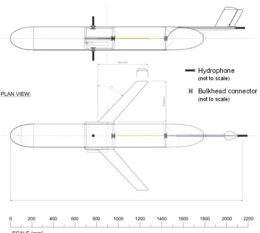
Figure 11: A glider with three hydrophones. Two hydrophones are fixed to the payload module.

(31)

(32)

(33)

(34)

E

Photos of glider, payload bay, hydrophones and

other electronics

Figure 15: An ocean glider that will be used to deploy the hydrophones.

Figure 16: A payload bay where all the electronic equipment used for sound source detec-tion will be mounted.

(35)

Figure 17: Marantz Professional PMD661 sound recorder used to record audio data from the hydrophones.

Figure 18: B&K 2634 charge amplifier used to amplify the audio signal from the hy-drophones.