HAL Id: hal-00427035
https://hal.archives-ouvertes.fr/hal-00427035v3
Submitted on 31 Mar 2010
HAL is a multi-disciplinary open access
archive for the deposit and dissemination of
sci-entific research documents, whether they are
pub-lished or not. The documents may come from
teaching and research institutions in France or
abroad, or from public or private research centers.
L’archive ouverte pluridisciplinaire HAL, est
destinée au dépôt et à la diffusion de documents
scientifiques de niveau recherche, publiés ou non,
émanant des établissements d’enseignement et de
recherche français ou étrangers, des laboratoires
publics ou privés.
Reconstructing Shapes with Guarantees by Unions of
Convex Sets
Dominique Attali, André Lieutier
To cite this version:
Dominique Attali, André Lieutier. Reconstructing Shapes with Guarantees by Unions of Convex Sets.
SoCG 2010 - 26th Annual Symposium on Computational Geometry, Jun 2010, Snowbird, Utah, United
States. pp.344-353, �10.1145/1810959.1811015�. �hal-00427035v3�
Reconstructing Shapes with Guarantees
by Unions of Convex Sets
∗[Extended Abstract]
†Dominique Attali
Gipsa-lab, Grenoble, France
[email protected]
André Lieutier
Aix-en-Provence, France
[email protected]
ABSTRACT
A simple way to reconstruct a shape A⊂ RN from a sample
P is to output an r-offset P + rB, where B ={x ∈ RN
| kxk ≤ 1} designates the unit Euclidean ball centered at the origin. Recently, it has been proved that the output P + rB is homotopy equivalent to the shape A, for a dense enough sample P of A and for a suitable value of the parameter r [12, 22]. In this paper, we extend this result and find convex sets C ⊂ RN, besides the unit Euclidean ball B, for which
P + rC reconstructs the topology of A. This class of convex sets includes in particular N -dimensional cubes in RN. We
proceed in two steps. First, we establish the result when P is an ε-offset of A. Building on this first result, we then consider the case when P is a finite noisy sample of A.
Categories and Subject Descriptors
F.2.2 [Analysis of Algorithms and Problem Complex-ity]: Nonnumerical Algorithms and Problems—Geometrical problems and computations, Computations on discrete struc-tures; I.3.5 [Computer Graphics]: Computational Geom-etry and Object Modeling
General Terms
Theory, Algorithms
Keywords
Shape reconstruction, offsets, Minkowski sum, union of con-vex sets, sampling, homotopy equivalence
∗This work is partially supported by ANR Project GIGA ANR-09-BLAN-0331-01.
†A full version of this paper is available at http://hal.archives-ouvertes.fr/hal-00427035
Permission to make digital or hard copies of all or part of this work for personal or classroom use is granted without fee provided that copies are not made or distributed for profit or commercial advantage and that copies bear this notice and the full citation on the first page. To copy otherwise, to republish, to post on servers or to redistribute to lists, requires prior specific permission and/or a fee.
SCG’10,June 13–16, 2010, Snowbird, Utah, USA. Copyright 2010 ACM 978-1-4503-0016-2/10/06 ...$10.00.
1.
INTRODUCTION
In this paper, we study the Minkowski sum between a convex set and a point set that samples a shape, generalizing previous results that establish the Minkowski sum retrieves the topology of the shape when the convex set is a Euclidean ball.
Prior work and problem.
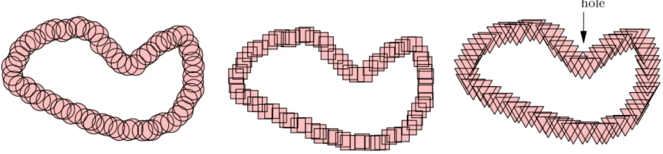
Motivated by surface reconstruction from 3D scan data and manifold learning from point clouds, several authors have formulated precise conditions under which a recon-struction algorithm outputs a topologically correct approxi-mation of a shape, given as input a possibly noisy sample of it [4, 14, 10, 22, 12]. Maybe one of the simplest algorithm consists in outputting a Euclidean r-offset of the sample, that is the union of Euclidean balls with radius r centered on the sample points. Assuming the reach of the shape is positive and data points form a sufficiently dense and accu-rate sample of the shape, authors in [22, 12] have established that r-offsets of the data points are homotopy equivalent to the shape for suitable values of the offset parameter r (see Figure 1, left). The aim of this work is to understand how this result generalizes when, instead of unions of Euclidean balls, we consider for the reconstruction unions of translated and scaled copies of a convex set C centered on the data points. In other words, writing B for the unit Euclidean ball centered at the origin and letting P be a sample of the shape A, we would like to understand what happens if we replace the Euclidean r-offset P + rB by the Minkowski sum P + rC. Do we keep the topology of the shape A as in Fig-ure 1, middle or do we lose it as in FigFig-ure 1, right? We are particularly interested in the case where C is a polytope.
Motivation.
Our motivation to study this question is two-fold. First, in many practical applications such as stereo vision or im-age analysis, the accuracy of measures varies in magnitude according to the direction of measurements. In this context, it seems reasonable to recover the topology of the shape, using a convex set which takes into account the anisotropy of the measurement device. Second, we believe that unions of cubes could present some advantages over unions of Eu-clidean balls for topological computations in high dimension. In practice, the reconstruction represented by an α-offset is replaced by the more convenient corresponding α-shape which shares the same homotopy type [15]. Indeed, the α-shape has a simpler geometry and, being a simplicial com-plex, can benefit from existing theorems and algorithms
ded-hole
Figure 1: The union of disks and squares retrieve the topology of the sampled curve unlike the union of triangles.
icated to topological computations. However, if the ambient dimension is large, the α-shape may have a high complex-ity [1] and its computation may be rather expensive and requires sophisticated data structures [8]. Our idea to cir-cumvent this problem is the following. Given ε > 0, we define the cubical grid Gε = (εZ)N ⊂ RN and replace the
sample P ⊂ RN by a nearby sample P
ε⊂ Gε. Applying our
result to the unit N -dimensional cube C = [−1, 1]N
∈ RN,
we shall see that the set Pε+ kεC retrieves the homotopy
type of the shape, for some well-chosen integer k. Hence, our result allows us to reconstruct with the right homotopy type a shape by a union of voxels with vertices the cubical grid (see [5] for a precise statement of this corollary and [6] for an application). Such a “cubical set” has a simpler structure than the α-shape and may be more convenient for topologi-cal computations in high dimension. Following this idea, our work might contribute to build a bridge between the point of view of distance functions in computational topology and the world of voxels in digital image processing.
Chosen approach and contributions.
A first idea to tackle the problem mentioned above is to use the framework of semi-concave functions. Specifically, one can associate to any symmetric convex set C with a non-empty interior a normk.kCdefined by x7→ kxkC = inf{α >
0| x ∈ αC}. The balls of the associated distance dC are
translated and scaled copies of C. The metric dCis invariant
by translation but is not isotropic unless C is the Euclidean ball. Suppose the boundary of C is smooth with a bounded curvature. Given a subset Y ⊂ RN, the squared
distance-to-Y function x7→ miny∈Ykx − yk2C is semi-concave [9] and
has therefore a generalized gradient which induces a contin-uous flow. Hence, a theory similar to what has been done in the Euclidean case [10, 11, 12] can be developed. However, we are interested in convex sets, such as polytopes, whose boundary are not necessarily smooth nor has a bounded cur-vature. It follows that the semi-concavity property is lost and no generalized gradient of the squared distance-to-Y function can induce a flow. The proof technique used in this paper should be of independent interest since it overcomes the limitation of flow-based methods and applies to convex sets with non-smooth boundary. Taking inspiration in [22] where a deformation retract of a Euclidean offset of the sam-ple onto the shape is constructed explicitly, we move away from this approach and introduce a new proof scheme based a sandwich lemma (Lemma 1). Results in this paper are positive as well as negative. We carefully identify a class of convex sets to which the above result can be extended. We
also give examples of convex sets outside this class which won’t provide a correct reconstruction. We proceed in two steps. First, we state a reconstruction theorem, when the sample P is an arbitrarily small Euclidean offset of the shape and secondly when P is a finite sample.
Outline.
Section 2 presents definitions and the formal statements of our two reconstruction theorems. Section 3 proves the first reconstruction theorem and Section 4 proves the second. Section 5 concludes the paper.
2.
STATEMENT OF RESULTS
Before we state our results in Section 2.3, we first intro-duce the necessary background in topology in Section 2.1 and identify in Section 2.2 classes of convex sets to which our results will apply.
2.1
Homotopy equivalences
First, we review some classical definitions in topology that can be found for instance in [18, 21]. Two continuous maps h, k : X → Y are homotopic and we write h ≃ k if there is a continuous map F : X× [0, 1] → Y such that F (x, 0) = h(x) and F (x, 1) = k(x) for all x ∈ X. Let f : X → Y and g : Y → X be two continuous maps. Suppose that f◦ g : Y → Y is homotopic to the identity map of Y and g◦ f : X → X is homotopic to the identity map of X, i.e. suppose we have f◦ g ≃ 1Y and g◦ f ≃ 1X. Then, the maps
f and g are called homotopy equivalences, and each is said to be a homotopy inverse of the other. Furthermore, the spaces X and Y are said to have the same homotopy type, which we denote by X ≃ Y . We say that a subspace A of X is a deformation retract of X if there exists a continuous map H : X× [0, 1] → X such that H(x, 0) = x, H(x, 1) ∈ A for all x∈ X and H(a, t) = a for all a ∈ A and all t ∈ [0, 1]. Such a function H is called a deformation retraction of X onto A. Let r : X→ A be the retraction defined by r(x) = H(x, 1) and let i : A → X the inclusion map. We have i◦ r ≃ 1Xand r◦ i = 1A. Thus, if A is a deformation retract
of X, the inclusion i : A → X is a homotopy equivalence. Note that assuming X deformation retracts to A is stronger than assuming the inclusion map A ֒→ X is a homotopy equivalence, which in turn is stronger than assuming A≃ X, as illustrated in Figure 2. We now state a technical lemma that will provide us key tools in establishing that two shapes have the same topology.
Figure 2: Two nested shapesA⊂ X which are close in Hausdorff distance and have the same homotopy type but for which the inclusion A ֒→ X is not a homotopy equivalence.
Lemma 1 (Sandwich Lemma). Consider four nested spaces A0 ⊂ X0 ⊂ A1 ⊂ X1. If A1 deformation retracts to
A0and X1deformation retracts to X0, then X0deformation
retracts to A0. If the inclusions A0 ֒→ A1 and X0 ֒→ X1
are homotopy equivalences, then the inclusion A0 ֒→ X1 is
a homotopy equivalence.
Proof. To prove the first part of the lemma, suppose F is a deformation retraction of A1 onto A0 and G is a
deformation retraction of X1 onto X0. Then, one can check
that the map H : X0× [0, 1] → X0 defined by H(x, t) =
G(F (x, t), 1) is a deformation retraction of X0 onto A0.
A0 j◦i0 > <... r ... A1 X0 <... s ... i1◦j > j > i0 > X1 i1 >
Figure 3: Diagram for the proof of Lemma 1. All arrows but the dotted ones are inclusions.
To prove the second part of the lemma, let i0: A0→ X0,
j : X0 → A1 and i1 : A1 → X1 denote inclusions (see
Figure 3). Suppose r is a homotopy inverse of j◦ i0 and s
is a homotopy inverse of i1◦ j. We prove that the inclusion
k = i1◦ j ◦ i0 from A0 to X1 is a homotopy equivalence
with homotopy inverse r◦ j ◦ s. Indeed, using the fact that composition preserves the relation≃, we have k ◦(r ◦j ◦s) = i1◦ (j ◦ i0◦ r) ◦ j ◦ s ≃ i1◦ 1A1◦ j ◦ s ≃ 1X1 and similarly
(r◦ j ◦ s) ◦ k = r ◦ j ◦ (s ◦ i1◦ j) ◦ i0≃ r ◦ j ◦ 1X0◦ i0≃ 1A0.
2.2
Properties on convex sets
In this section, we define two properties that will help us identify classes of convex sets.
2.2.1
θ-roundness
We associate to every compact convex set a non-negative real number called the θ-roundness which can be interpreted as a certain kind of curvature. Given a convex set C in RN,
the normal coneN (x) to C at x is the set of unit vectors n such that (x− y) · n ≥ 0, for all points y ∈ C.
Definition 1. Let θ ∈ [0, π] and κ ≥ 0. We say that the compact convex set C is (θ, κ)-round if for all points c1, c2∈ C and all vectors n1 ∈ N (c1) and n2 ∈ N (c2), the
following implication holds:
∠(n1, n2)≥ θ =⇒ (c1− c2)· (n1− n2)≥ κ kc1− c2k2.
The θ-roundness of C is the supremum of κ ≥ 0 such that C is (θ, κ)-round.
Note that if the compact convex set C has θ-roundness κ, then C is (θ, κ)-round. If C is (θ, κ)-round, then C is (θ′, κ′)-round whenever θ≤ θ′and κ′≤ κ. It is not difficult
to see that C is (π, κ)-round if and only if the diameter of C is upper bounded by 2
κ. Suppose the boundary of C is a C 2
-smooth hypersurface in RNand orient ∂C such that normals
point outside the convex set. Then, for all points x∈ ∂C, the normal cone at x is reduced to a single vector which is the normal to ∂C at x. The absolute values of the principal curvatures at point x ∈ ∂C are non-negative real numbers |κ1(x)| ≥ |κ2(x)| . . . ≥ |κN −1(x)| and we let κmin(C) be the
minimum of|κN −1(x)| over all points x ∈ ∂C.
Lemma 2. A compact convex set C whose boundary is C2-smooth has 0-roundness κmin(C).
See Appendix B for a proof. For our reconstruction the-orems, we shall consider compact convex sets which have the property to be (θ, κ)-round for a positive κ and a small enough θ. Specifically, we will require θ≤ θN= arccos(−N1).
Not all convex sets satisfy this property. To construct a counterexample, consider a compact convex set C which is contained in an affine space of dimension i with 0 < i < N . Let n be a unit vector orthogonal to the smallest affine space containing C. For every point c ∈ C, both n and its op-posite vector −n belong to N (c). Consider two distinct points c1, c2 ∈ C and let n1 = n and n2 =−n. We have
∠(n1, n2) = π, (c1− c2)· (n1− n2) = 0 and kc1− c2k 6= 0,
showing that there are no κ > 0 such that C is (π, κ)-round. Equivalently, the π-roundness of C is zero. As a counterex-ample with a non-empty interior, take a triangular prism in R3. Its θ3-roundness is zero. In the technical report [5], we compute the θ2-roundness of regular polygons in the plane
and establish that the θN-roundness of the N -dimensional
cube B∞= [−1, 1]N⊂ RN is: κ(B∞) = 8 > < > : 1 2√2`cos π 4 + cos π 12 ´ if N = 2, 1 √ 6 if N = 3, 1 (N −2)√N if N≥ 4,
2.2.2
Eccentricity
In this section, we associate to every subset C ⊆ RN a
parameter called eccentricity. Intuitively, eccentricity can be thought of as a measure of how much intersections of translated copies of C centered at points in Q deviate from the convex hull of Q. We recall that the Minkowski sum of two subsets X ⊂ RN and Y
⊂ RN is the subset defined by
X + Y ={x + y | x ∈ X, y ∈ Y }. To simplify notations, we shall write x + Y instead of {x} + Y . Let B = {x ∈ RN
| kxk ≤ 1} be the unit Euclidean ball centered at the origin. Given a non-negative real number r, we call the Minkowski sum X + rB the Euclidean r-offset of X and denote it by Xr. We write Conv(Q) for the convex hull of Q
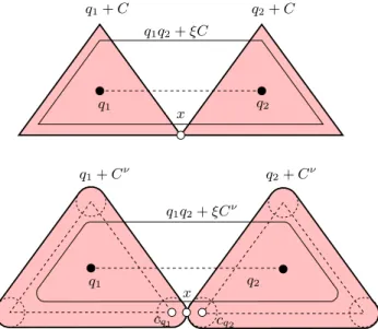
Definition 2. Given ξ≥ 0, we say that C is ξ-eccentric if for all compact Q⊂ RN, the following implication holds
(see Figure 4): \ q∈Q (q + C)6= ∅ =⇒ \ q∈Q (q + C) ! ∩ (Conv(Q) + ξC) 6= ∅. The eccentricity of C is the infimum of ξ ≥ 0 such that C is ξ-eccentric. cq1 cq2 q2 q1 q1+ C q2+ C q1q2+ ξC x q1 q1+ Cν q2+ Cν q2 x q1q2+ ξCν
Figure 4: Top: two translated copies of a triangleC. The intersection pointx does not belong to any set Conv({q1, q2})+ξC for ξ < 1, thus showing that the
ec-centricity is 1. Bottom: bulging the triangle makes its eccentricity drops to a value smaller than 1.
Note that the eccentricity is a real number between 0 and 1. If the eccentricity of a compact set C is ξ, then C is ξ-eccentric. The property to be ξ-eccentric is invariant under bijective linear transformations. We now give eccentricities for simple objects and adopt the convention that all objects we consider in this paragraph have their centroids at the ori-gin. Computations can be found in the technical report [5]. The eccentricity of the unit N -dimensional Euclidean ball B is zero. More generally, i-dimensional Euclidean balls for 0 ≤ i ≤ N have eccentricity 0. Ellipsoids which can be obtained from Euclidean balls by applying a linear transfor-mation also have eccentricity 0. Symmetric compact convex sets in the plane have eccentricity 0 as well. At the oppo-site end of the spectrum, triangles have eccentricity 1 (see Figure 4). In [5], we show that N -dimensional cubes have eccentricity 1− 2
N, for N≥ 2.
2.3
Reconstruction Theorems
First, we formulate a sampling condition inspired by the work in [2, 3, 10]:
Definition 3. Given a non-negative real number ε and a subset C⊂ RN, we say that P
⊂ RN is an (ε, C)-sample
of A⊂ RN if A
⊂ P + εC and P ⊂ A + εB.
Notice that P is an (ε, B)-sample of A if and only if the Hausdorff distance between P and A does not exceed ε. If
B⊂ C, then an (ε, B)-sample is also an (ε, C)-sample. The reason why our definition is not symmetric with respect to A and P is to enhance conditions that are used in the proofs of our reconstruction theorems. Given a compact subset A of RN, we recall that the medial axis M of A is the set of
points in RN which have at least two closest points in A.
The reach of A is the infimum of distances between points in A and points in M :
reach(A) = inf
a∈A,x∈Mka − xk.
Shapes with a positive reach include, but are not limited to, compact smooth surfaces with bounded curvatures. In-tuitively, a shape with a positive reach cannot have sharp concave edges. Suppose A has a positive reach. Given a convex set C and an (ε, C)-sample P of A, we would like to know whether the Minkowski sum P +rC retrieves the topol-ogy of A. Theorem 1 answers the question when P = Aε is
a Euclidean ε-offset of A and Theorem 2 provides an answer when P is a finite sample of A. Before stating our results, we start with an example which illustrates that not all con-vex sets C can be used to reconstruct the topology of shapes with a positive reach.
Figure 5: Cycle in the Minkowski sum of the mo-ment curve with a segmo-ment.
Specifically, we take A to be the moment curve A = {(x1, x2, x3) ∈ R3 | x2 = x21, x3 = x31} and prove that
for r arbitrarily small, we can always find a convex set C such that the Minkowski sum A + rC is not homotopy equivalent to A. For this, let C be a segment of length 2 centered at the origin and contained in the straight-line Lt = {(x1, x2, x3) ∈ R3 | x2 = 0, x3 = t2x1} for some
positive real number t. Observe that translated copies of Lt intersect the moment curve A in at most one point,
ex-cept when the translated copy meets A in the two points at= (t, t2, t3) and bt = (−t, t2,−t3). Hence, as r increases,
the Minkowski sum A + rC undergoes a topology change when the two segments at+ rC and bt+ rC meet (see
Fig-ure 5). This happens for r =kat− btk/2 which can be made
arbitrarily small by choosing t small enough. We now list conditions we shall need on the compact convex set C, the last condition being only for the second theorem:
(i) B⊂ C ⊂ δB for some δ ≥ 1;
(ii) C is (θ, κ)-round for θ≤ θN= arccos(−N1) and κ > 0;
(iii) C is ξ-eccentric for ξ < 1.
The two conditions (ii) and (iii) do not imply each other. Indeed, any equilateral triangle in R2 with centroid the
ori-gin has eccentricity 1 and a positive θ-roundness for all 0 < θ ≤ θ2. Hence, it satisfies (ii) for some θ ≤ θ2 and
some κ > 0 but not (iii) for any ξ < 1. Conversely, a seg-ment in R2has θ
satisfies (iii) for ξ = 0 but not (ii) for any θ≤ θ2and κ > 0.
Table 1 gathers for different compact convex sets C values of δ, θ, κ and ξ for which conditions (i), (ii) and (iii) hold. To state our theorems, let us introduce:
Rr = R−r 4− r r 4 “ 2R +r 4 ” , and note that Rrtends to R as Rr → 0.
Theorem 1. Let A be a compact subset of RN with
pos-itive reach R. Let C be a compact convex set of RN
satis-fying conditions (i) and (ii). Then, Aε+ rC deformation
retracts to A for all real numbers ε > 0 and r > 0 such that ε + (δ− 1)r < min{R − r, Rr/κ}.
The proof of Theorem 1 is given in Section 3. Theorem 1 will be useful in establishing our second theorem:
Theorem 2. Let A be a compact subset of RN with posi-tive reach R. Let C be a compact convex set of RNsatisfying
conditions (i), (ii) and (iii). Let P be a finite (ε, C)-sample of A. Then, the inclusion A ֒→ P + rC is a homotopy equiv-alence for all real numbers ε > 0 and r > 0 such that (1) (δ−1)r < min{R−r, Rr/κ}, (2) δr < R−ε, (3) δ(r+α0) < R
and (4):
2R−p(R − ε)2− (δr)2−pR2− δ2(r + α0)2< (1−ξ)r −ε,
where α0= ξr + R−p(R − ε)2− (δr)2.
The proof of Theorem 2 is given in Section 4. Notice that Theorem 2 requires that θ ≤ θN, κ > 0 and ξ < 1. If
these three conditions are fulfilled, then by choosing r =
4ε 1−ξ and
ε
R small enough, all the assumptions of Theorem 2
are satisfied, implying that the inclusion A ֒→ P + rC is a homotopy equivalence. Given a fixed convex set C, Table 1 gives numerical approximations of the largest value of Rε for which assumptions of Theorem 2 hold.
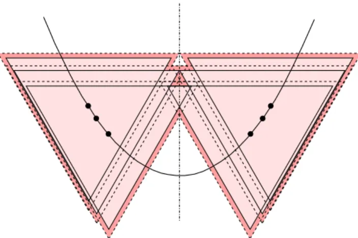
To conclude this section, we prove that condition (iii) in Theorem 2 is necessary. In other words, if we take a com-pact convex set C which satisfies conditions (i) and (ii) but whose eccentricity is 1, it may happen that for some sample P , the Minkowski sum P + rC does not recover the topology of A, no matter what value r takes in the interval [ε, R− ε]. To construct such an example, consider a parabola A in the plane with equation y = x2and a finite sample P ⊂ A sym-metric with respect to the y-coordinate axis. Furthermore, we let C be the equilateral triangle with centroid the origin and vertices (0,−2), (√3, 1) and (−√3, 1). We note that with increasing value of r, holes appear in the Minkowski sum P + rC each time two triangles scaled by r meet at a common vertex on the y-axis (see Figure 6). We then adjust the height of the sample points in such a way that P + εC does not have the correct topology and as r increases, a hole appears in P + rC each time a hole gets destroyed, as illustrated in Figure 6.
3.
PROOF OF THEOREM 1
In this section, we prove Theorem 1. In other words, we prove that for r and ε small enough with respect to the reach of A, the Minkowski sum Aε+ rC deformation retracts to
A. Our strategy is as follows. We consider two positive real numbers ε′and ε′′such that there is chain of inclusions:
A ⊂ Aε+ rC ⊂ Aε′ ⊂ Aε′′+ rC (1)
Figure 6: As the size of triangles increases, the hole created by the 4 upper points appears exactly when the hole created by the 4 lower points fills up.
and find conditions under which the third set deformation re-tracts to the first set and the fourth set deformation rere-tracts to the second set. Applying the Sandwich Lemma allows us to conclude. All the difficulty comes from the second part of the proof which involves comparing the topology of two Eu-clidean offsets of A+rC, namely Aε+rC and Aε′′+rC. This leads us to study in details Euclidean offsets of Minkowski sums in Section 3.2. A powerful tool for detecting changes in the topology of Euclidean offsets consists in studying the critical points of distance functions. Key results concerning distance functions are recalled in Section 3.1.
3.1
Background on distance functions
The distance function d(·, Y ) to the compact subset Y of RN associates to each point x
∈ RN its Euclidean
dis-tance to Y , d(x, Y ) = miny∈Ykx − yk. The distance
func-tion d(·, Y ) is 1-Lipschitz, but is not differentiable in gen-eral. Nonetheless, it is possible to define a notion of crit-ical points analogue to the classcrit-ical one for differentiable functions. Specifically, Grove defines in [17, page 360] crit-ical points for the distance function to a closed subset of a Riemannian manifold. Using Equation (1.1)’ in [17, page 360], we recast this definition in our context as follows. Let ΓY(x) ={y ∈ Y | d(x, Y ) = kx − yk} be the set of points in
Y closest to x:
Definition 4. A point x∈ RN is a critical point of the
distance function d(·, Y ) if x ∈ Conv(ΓY(x)). The
criti-cal values of d(·, Y ) are the images by d(·, Y ) of its critical points.
Slightly recasting Proposition 1.8 in [17, page 362], we have:
Lemma 3 (Isotopy Lemma [17]). Let 0 < ε≤ ε′. If
the distance function d(·, Y ) has no critical value in the in-terval [ε, ε′], then Yε is a deformation retract of Yε′
. If furthermore Y has a positive reach R, then the pro-jection map πY which associates to each point x ∈ Yε its
closest point πY(x) on Y is well defined and continuous [16,
page 435]. Thus, the map H : [0, 1]× Yε
→ Yε defined by
H(t, x) = (1− t)x + tπY(x) is a deformation retraction of
Table 1: Columns2 to 5: values of δ, θ, κ and ξ for which B⊂ C ⊂ δB and the convex set C is (θ, κ)-round and ξ-eccentric. Columns 6 and 7: values of R/ε and r/ε for which Theorem 2 holds. Numerical values are obtained by brute force, enumerating all pairs(ε, r) in a grid, checking if they satisfy conditions of Theorem 2 and keeping the one with largestε.
convex set C δ θ κ ξ R/ε r/ε Euclidean ball B⊂ RN 1 0 1 0 12.9781 3.95723 cube B∞in RN √N arccos(−N1) κ(B∞) 1 −N2 cube B∞in R2 √2 2π3 0.65974 0 24.9973 4.04227 cube B∞in R3 √ 3 0.608 π √1 6 1/3 96.4687 6.14485 cube B∞in R4 √ 4 0.5804 π 1/4 1/2 247.528 8.1826 cube B∞in R5 √5 0.5641 π 0.149071 3/5 508.183 10.2006 cube B∞in R10 √10 0.5319 π 0.03953 4/5 4505.44 20.2264 cube B∞in R100 10 0.503183 π 0.0010204 49/50 4948245 200.232
p-gonPp in R2 (p even) cos1π p 2π 3 κ(Pp) 0 square in R2 √2 2π3 0.65974 0 24.9973 4.04227 hexagon in R2 1.1547 2π 3 0.69936 0 16.9858 3.99837 octagon in R2 1.08239 2π 3 0.793353 0 15.04119 3.98101 dodecagon in R2 1.03528 2π 3 0.8660254 0 13.84148 3.968 36-gon in R2 1.00382 2π 3 0.951917 0 13.07011 3.95844 360-gon in R2 1.00004 2π 3 0.9949868 0 12.97897 3.95724
Lemma 4. If Y has a positive reach R, then Yε deforma-tion retracts to Y , for all 0≤ ε < R.
3.2
Distance functions to Minkowski sums
In what follows, A designates a compact subset of RNwith
positive reach R and C designates a compact convex set of RN. We begin with a technical lemma which will help us to situate critical points of the distance function to A + C, assuming C is round enough.
Lemma 5. Consider a point x∈ RN such that d(x, A +
C) < R. Let y1, y2 ∈ ΓA+C(x) be two points on A + C
with minimum distance to x. Suppose C is (θ, κ)-round for κ> 0 and ∠y1xy2≥ θ. Then, d(x, A + C) ≥ R
1/κ.
Figure 7: Notations for the proof of Lemma 5. Proof. Let ρ = d(x, A+C). For i∈ {1, 2}, let yi= ai+ci
with ai∈ A and ci∈ C. Since ρ = k(x − ci)− aik < R, it
follows that x− ci has a unique projection ai= πA(x− ci)
onto A (see Figure 7). On the other hand, we know from [16, page 435] that the projection map πAonto A is
“
R R−ρ
” -Lipschitz for points at distance less than ρ from A. Thus,
ka1− a2k ≤ R
R− ρkc1− c2k. Let ni = kx−ax−ai−ci
i−cik. Squaring both sides of the above
in-equality and plugging a2− a1 = c1− c2+ ρ(n1− n2) into
the left side, we obtain
2(c1− c2)· (n1− n2) + ρkn1− n2k2 ≤
2R− ρ
(R− ρ)2kc1− c2k 2.
For i∈ {1, 2}, the unit vector nibelongs toN (ci). Since C
is (θ, κ)-round and ∠(n1, n2)≥ θ, it follows that (c1− c2)·
(n1− n2)≥ κkc1− c2k2 and ρkn1− n2k2≤ „ 2R− ρ (R− ρ)2 − 2κ « kc1− c2k2.
In particular, this implies that 2κ≤(R−ρ)2R−ρ2 or equivalently
ρ2
− 2`R − 1
4κ´ ρ + R 2
− R
κ ≤ 0. Solving this quadratic
inequality yields to the result.
As a consequence of the lemma above, if x is sufficiently close to A + C, then the angle between any two vectors connecting x to points in ΓA+C(x) is small which implies,
in turn, that x is not a critical point of d(·, A + C). The following lemma makes this idea precise.
Lemma 6. If C is (θ, κ)-round with θ≤ arccos(−1 N) and
κ> 0, then the distance function d(·, A + C) has no critical value in the interval (0, R1/κ).
In order to prove Lemma 6, we need the following result also known as Jung’s Theorem. Given a compact subset K ⊂ RN, we denote by diam(K) = max
p,q∈Kd(p, q) the
diameter of K.
Lemma 7 (Jung’s Theorem). The smallest ball enclos-ing a compact subset K of RN has radius
r≤ diam(K) s
N 2(N + 1). Equality is attained for the regular N-simplex.
Proof of Lemma 6. Let x∈ RN and ρ = d(x, A + C).
Suppose 0 < ρ < R1/κ and let us prove that x is non-critical. By Lemma 5, for all points y1, y2 ∈ ΓA+C(x), we
have ∠y1xy2< θ. It follows that diam(ΓA+C(x)) < 2ρ sinθ2.
Using sinθ 2 = r 1− cos θ 2 ≤ r N + 1 2N ,
and applying Jung’s Theorem, we get that the smallest ball B enclosing ΓA+C(x) has radius r < ρ. Let S denote the
sphere centered at x with radius ρ. Observe that ΓA+C(x)⊂
S∩ B. Since the radius of B is smaller than ρ, the rad-ical hyperplane Π of the two spheres S and ∂B separates x from ΓA+C(x). Thus x6∈ Conv(ΓA+C(x)) and x is
non-critical.
Combining Lemma 3 and Lemma 6 and using the fact that if C is (θ, κ)-round, then rC is (θ,κ
r)-round, we get
immediately conditions under which a Euclidean offset of A + rC deformation retracts to another Euclidean offset:
Lemma 8. If C is (θ, κ)-round with θ≤ arccos(−1 N) and
κ> 0, then Aε+ rC is a deformation retract of Aε′′+ rC for all positive real numbers r, ε and ε′′such that ε≤ ε′′<
Rr/κ.
We are now ready to establish the proof of our first recon-struction theorem.
Proof of Theorem 1. Equation (1) holds whenever ε′=
ε + δr and ε′′= ε + (δ− 1)r. Since by hypothesis ε ≤ ε′′<
Rr/κ, Lemma 8 implies that Aε
′′
+ rC deformation retracts to Aε+ rC. By hypothesis, we have ε′ < R and therefore,
Aε′
deformation retracts to A from Lemma 4. Applying the Sandwich Lemma allows us to conclude.
4.
PROOF OF THEOREM 2
In this section, we present our proof of Theorem 2. A designates a compact subset of RNwhose reach R is positive,
C is a compact convex set of RN satisfying conditions (i), (ii) and (iii) and P is a finite (ε, C)-sample of A. First, we introduce a set which will play a key role. Given three positive real numbers α, β and r, we setAp(α) = (p + rC)∩
(Aβ+ αC) and define H(α) = [
p∈P
ConvAp(α).
Our proof uses two carefully chosen positive constants α0
and α1 such that for all sufficiently small β, we have the
sequence of inclusions (see Figure 8):
A ⊂ H(α0) ⊂ Aβ+ α1C ⊂ P + rC (2)
Having established this sequence of inclusions in Section 4.1, we find in Section 4.2 conditions under which H(α0) ֒→
P + rC is a homotopy equivalence. Combined with the conditions we found in Section 3 which ensure that A ֒→ Aβ+ α1C is a homotopy equivalence, we deduce
immedi-ately using Lemma 1 (Sandwich Lemma) conditions under which A ֒→ P + rC is a homotopy equivalence.
4.1
Establishing a key sequence of inclusions
In this section, we find conditions under which inclusions in (2) hold. To establish the middle inclusion, we need the following key inclusion, illustrated in Figure 8:
Conv Aq(α0) q A Conv Ap(α0) p Aβ+ α 0C P + rC Aβ+ α1C C
Figure 8: Nested sequence of objects considered for the proof of Theorem 2. Constants α0 and α1 are
chosen such thatConvAp(α0) is contained in A + α1C
for all p∈ P .
Lemma 9. Suppose δ(r + α0) < R− β and α1− α0 ≥
R−p(R − β)2− δ2(r + α0)2. Then,
ConvAp(α0) ⊂ A + α1C.
Proof. Let A′ = Aβ ∩ (p + rC + α0(−C)). Note that
Ap(α0)⊂ A′+ α0C for if x belongs toAp(α0) = (p + rC)∩
(Aβ+ α
0C), we can find c0, c1 ∈ C and a′ ∈ Aβ such that
x = a′+ α0c0 = p + rc1, showing that a′ ∈ A′ and x ∈
A′+ α0C. Thus and using lemma 15,
ConvAp(α0) ⊂ Conv(A′+ α0C) = Conv(A′) + α0C.
By construction, A′is contained in a ball of radius δ(r +α 0).
Applying Lemma 14 with Q = A′, ε = β and ρ = δ(2r− ε), we get
Conv(A′) ⊂ A + (R −p(R − β)2− ρ2)B
if ρ < R− β. Thus, for all p ∈ P we have Conv Ap(α0)⊂
A + α1C whenever δ(r + α0) < R− β and α1− α0 ≥ R −
p(R − β)2− δ2(r + α 0)2.
Taking the union over all points p∈ P on both sides of the inclusion in Lemma 9 we get immediately the middle inclusion in (2), i.e. H(α0) ⊂ Aβ+ α1C. The left-most
and right-most inclusions in (2) are easy to establish, using A⊂ P + εC and B ⊂ C.
Lemma 10. The sequence of inclusions in (2) holds when-ever α1 ≤ r − ε − β, δ(r + α0) < R− β and α1− α0 ≥
R−p(R − β)2− δ2(r + α0)2.
4.2
A homotopy equivalence for nested
collec-tions of convex sets
It is not difficult to see that the inclusionH(α) ⊂ P + rC holds for all positive real numbers α and β. The goal of this section is to find conditions under which the inclusion map H(α) ֒→ P +rC is a homotopy equivalence. For this, we use covers of H(α) and P + rC by finite collections of convex sets. Specifically, we have H(α) = S
p∈PConvAp(α) and
P + rC =S
p∈P(p + rC). Since sets in the two collections
{Conv Ap(α)}p∈P and{p+rC}p∈Pare convex, we can apply
Leray’s theorem [20] to each, and obtain that the union of sets in each collection has the same homotopy type as its associated nerve:
H(α) ≃ Nerve{Conv Ap(α)}p∈P
A key step consists in proving that, for suitable values of α, the nerves of the two collections are actually the same. As a consequence,H(α) and P + rC have the same homotopy type. We strengthen this result thanks to Lemma 11: and state conditions under which the inclusionH(α) ֒→ P + rC is a homotopy equivalence in Lemma 12.
Lemma 11. Consider two finite collections of compact con-vex sets of RN,
C = {Ci}i∈I and D = {Di}i∈I such that
Ci⊂ Di for all i∈ I and suppose the two collections have
the same nerve. Then, the inclusionS
iCi ֒→ SiDi is a
homotopy equivalence.
From Corollary 4G.3 in [18] also known as Leray’s the-orem [20] or the Nerve Lemma, it is clear thatS
iCi and
S
iDiwhich share the same nerve have the same homotopy
type. But, we need here a stronger result, namely that the inclusionS
iCi ֒→SiDi is a homotopy equivalence. Even
though this fact can be deduced from a result in [7], we pro-vide below a short proof to make the paper self-contained.
Proof. Let K(C) be the abstract simplicial complex whose simplices are the (non-empty) subsets of indices σ⊂ I such thatT
i∈σCi 6= ∅. Since the two collections C and D have
the same nerves, K(C) = K(D) and we let K = K(C). For every subset of indices σ /∈ K, a standard compactness argument yields a real number ρσ > 0 such thatTi∈σDρiσ =
∅. Let ρ = minσ /∈Kρσ and define the open set Oi ={x ∈
RN, d(x, Di) < ρ} for every i ∈ I. By construction, the nerve of the collectionO = {Oi}i∈I is the same as the nerve
of D and K(O) = K. For each σ ∈ K, we introduce the possibly empty open set:
Uσ= \ i∈σ Oi\ [ i /∈σ Di.
It is obvious from the definition thatS
σ∈KUσ ⊂
S
i∈IOi.
Let us associate to each point x ∈ S
i∈IOi the subset of
indices τ (x) ={i ∈ I, x ∈ Oi}. Since x ∈ Uτ (x), it follows
that: [ σ∈K Uσ= [ i∈I Oi.
Let us consider a partition of unity{φσ}σ∈K subordinate to
the open cover{Uσ}σ∈K [23, page 22]. Note that the map
φσ is identically zero for the simplices σ for which Uσ =∅.
For each simplex σ∈ K, we choose an arbitrary point cσ∈
T
i∈σCi and introduce the map h :
S i∈IDi→ R N defined by: h(x) = X σ∈K φσ(x)cσ.
By construction, h is continuous. We claim that x∈ Di =⇒
h(x)∈ Ci. Indeed, if x∈ Diand φσ(x)6= 0, one has i ∈ σ
and therefore cσ ∈ Ci. Hence, the non-zero terms in the
above sum is a convex combination of points in Ciand the
claim follows from the convexity of Ci. Let us prove that h is
a homotopy inverse of the inclusion map g :S
iCi→
S
iDi.
In other words, we have to check that g◦ h is homotopic to the identity ofS
iDiand h◦g is homotopic to the identity of
S
iCi. This can be done using twice the homotopy H(x, t) =
(1−t)·x+t·h(x), first considered as a map fromS
iDi×[0, 1]
intoS
iDi, second considered as a map from
S
iCi× [0, 1]
intoS
iCi.
Lemma 12. Consider positive real numbers r, ε, α and β such that δr < R− ε, δ(r + α) < R − β and α ≥ ξr + R − p(R − ε)2− (δr)2. Then, the inclusionH(α) ֒→ P + rC is
a homotopy equivalence.
Proof. We prove the lemma in three stages:
(a) First, we prove that for δr < R− ε and α ≥ ξr + R − p(R − ε)2− (δr)2, we have
Nerve{p + rC}p∈P = Nerve{Ap(α)}p∈P. (3)
Note that this is equivalent to proving that for all subsets Q⊂ P , \ q∈Q (q + rC)6= ∅ ⇐⇒ \ q∈Q [(q + rC)∩ (Aβ+ αC)]6= ∅.
One direction is trivial: if a point belongs to the intersection on the right, then it belongs to the intersection on the left. Suppose now thatT
q∈Q(q + rC)6= ∅. In particular, using
C⊂ δB this means that Q can be enclosed in a ball of radius ρ = δr. Since C is ξ-eccentric, there exists z∈T
q∈Q(q +rC)
such that z∈ Conv(Q) + ξrC. Since P is an (ε, C)-sample of A, we have Q⊂ P ⊂ Aε. Applying Lemma 14, we get
that Conv(Q) ⊂ Aα−ξr. Hence and using B ⊂ C, we get
z∈ A + (α − ξr)B + ξrC ⊂ Aβ+ αC.
(b) Second, we prove that
Nerve{p + rC}p∈P = Nerve{Conv Ap(α)}p∈P. (4)
From Lemma 9, we obtain the sequence of inclusions Ap(α) ⊂ Conv Ap(α) ⊂ Ap(α′),
for δ(r+α) < R−β and α′= α+R−p(R − β)2− δ2(r + α)2.
Taking the intersection over all points q∈ Q, we get \ q∈Q Aq(α) ⊂ \ q∈Q ConvAq(α) ⊂ \ q∈Q Aq(α′), and consequently
Nerve{Ap(α)} ⊂ Nerve{Conv Ap(α)} ⊂ Nerve{Ap(α′)},
where p ranges over P . By Equation (3), the two nerves on the left and on the right are equal to Nerve{p + rC}p∈P,
showing that Nerve{Conv Ap(α)}p∈P = Nerve{p + rC}p∈P.
(c) Third, noticing that ConvAp(α) ⊂ p + rC for all p,
we apply Lemma 11 to the two collections of convex sets C = {Conv Ap(α)}p∈P andD = {p + rC}p∈P.
We conclude this section by the proof of our second re-construction theorem.
Proof of Theorem 2. For β small enough, we have β + (δ− 1)r < min{R − r, Rr/κ}, δ(r + α0) < R− β and
2R−p(R − ε)2− (δr)2−p(R − β)2− δ2(r + α 0)2
≤ (1 − ξ)r − ε − β. Setting α1= α0+ R−p(R − β)2− δ2(r + α0)2, the above
inequality can be rewritten as α1≤ r − ε − β. Thus, the
se-quence of inclusions in (2) holds by Lemma 10. Furthermore, the inclusionH(α) ֒→ P + rC is a homotopy equivalence by Lemma 12. Since α1≤ r and β+(δ−1)r < min{R−r, Rr/κ}
imply β + (δ− 1)α1 < min{R − α1, Rα1/κ}, the inclusion
A ֒→ Aβ+ α
1C is a homotopy equivalence by Theorem 1.
5.
DISCUSSION
In this paper, we have exhibited a class of compact convex sets whose Minkowski sum with a sufficiently dense sample retrieves the topology of the sampled shape. Compact con-vex sets in this class possess three properties: a non-empty interior, a positive θN-roundness and an eccentricity smaller
than 1. In particular, this class contains Euclidean balls but, more interestingly, also includes N -dimensional cubes, with potential algorithmic applications in high dimensions.
Results in this paper raise a number of questions. For instance, it would be interesting to know what is the lowest density of sample points Theorem 2 authorizes and if this number is tight, especially for N -dimensional balls. Also, Theorem 2 requires the sample P to be finite and the shape A to have a positive reach. Can we relax these two condi-tions?
6.
REFERENCES
[1] N. Amenta, D. Attali, and O. Devillers. A tight bound for the Delaunay triangulation of points on a pol yhedron. Research Report 6522, INRIA, May 2008. [2] N. Amenta and M. Bern. Surface reconstruction by
Voronoi filtering. Discrete and Computational Geometry, 22(4):481–504, 1999.
[3] N. Amenta, S. Choi, T. Dey, and N. Leekha. A simple algorithm for homeomorphic Surface Reconstruction. International Journal of Computational Geometry and Applications, 12:125–141, 2002.
[4] N. Amenta, S. Choi, and R. Kolluri. The power crust, unions of balls, and the medial axis transform. Computational Geometry: Theory and Applications, 19(2-3):127–153, 2001.
[5] D. Attali and A. Lieutier. Reconstructing shapes with guarantees by unions of convex sets. Archive Hal, hal-00427035, 2009.
[6] D. Attali and A. Lieutier. Optimal reconstruction might be hard. In 26th Ann. Sympos. Comput. Geom., Snowbird, Utah, 2010.
[7] P. Bendich, D. Cohen-Steiner, H. Edelsbrunner, J. Harer, and D. Morozov. Inferring local homology from sampled stratified spaces. In Proc. 48th Ann. Sympos. Found. Comput. Sci., pages 536–546, 2007. [8] J.-D. Boissonnat, O. Devillers, and S. Hornus.
Incremental construction of the Delaunay triangulation and the Delaunay graph in medium dimension. In Proc. ACM Symposium on
Computational Geometry, June 2009.
[9] P. Cannarsa and C. Sinestrari. Semiconcave functions, Hamilton-Jacobi equations, and optimal control. Birkhauser, 2004.
[10] F. Chazal, D. Cohen-Steiner, and A. Lieutier. A sampling theory for compact sets in Euclidean space. Discrete and Computational Geometry, 41(3):461–479, 2009.
[11] F. Chazal and A. Lieutier. The λ-medial axis. Graphical Models, 67(4):304–331, 2005. [12] F. Chazal and A. Lieutier. Smooth Manifold
Reconstruction from Noisy and Non Uniform Approximation with Guarantees. Computational Geometry: Theory and Applications, 40:156–170, 2008.
[13] V. de Silva and R. Ghrist. Coverage in sensor networks via persistent homology. Algebraic & Geometric Topology, 7:339–358, 2007.
[14] T. Dey, J. Giesen, E. Ramos, and B. Sadri. Critical points of the distance to an epsilon-sampling of a surface and flow-complex-based surface reconstruction. In Proc. of the twenty-first annual symposium on Computational geometry, page 227. ACM, 2005. [15] H. Edelsbrunner. The union of balls and its dual
shape. Discrete Computational Geometry, 13(1):415–440, 1995.
[16] H. Federer. Curvature measures. Trans. Amer. Math. Soc, 93:418–491, 1959.
[17] K. Grove. Critical point theory for distance functions. In Proc. of Symposia in Pure Mathematics, volume 54, pages 357–386, 1993.
[18] A. Hatcher. Algebraic topology. Cambridge University Press, 2002.
[19] D. Koutroufiotis. On Blaschke’s rolling theorems. Archiv des Mathematik, 23(1):655–660, 1972.
[20] J. Leray. Sur la forme des espaces topologiques et sur les points fixes des repr´esentations. J. Math. Pures Appl., 24:95–167, 1945.
[21] J. R. Munkres. Topology. Prentice Hall, 2000. [22] P. Niyogi, S. Smale, and S. Weinberger. Finding the
Homology of Submanifolds with High Confidence from Random Samples. Discrete Computational Geometry, 39(1-3):419–441, 2008.
[23] L. Schwartz. Th´eorie des distributions. Hermann, Paris, 1966.
APPENDIX
A.
BASIC PROPERTIES
In this appendix, we present basic properties relating the smallest ball enclosing Q⊂ RN and the convex hull of Q.
Lemma 13. Consider a subset Q ⊂ RN whose smallest
enclosing ball has radius r. Then, Conv(Q)⊂S
q∈QB(q, r).
Proof. For all q∈ Conv(Q), there are points q1, . . . , qn
in Q and non-negative real numbers α1, . . . , αnsumming up
to 1, such that q =Pn
i=1αiqi. Let πi(x) =kx − qik2− r2 be
the power distance of x∈ RN from B
i = B(qi, r) and note
that Bi = π−1i (−∞, 0]. Let π(x) =
Pn
i=1αiπi(x) and set
B = π−1(−∞, 0]. We prove thatTn
i=1Bi ⊂ B ⊂
Sn i=1Bi.
Indeed, if a point x belongs to all balls Bi, then πi(x)≤ 0
for all 1 ≤ i ≤ n, which implies π(x) ≤ 0. On the other hand, if π(x) ≤ 0 then πi(x)≤ 0 for at least one index i,
which implies that x belongs to at least one ball Bi. Now,
our choice of r as the radius of the smallest ball enclosing Q implies thatTn
i=1Bi6= ∅, showing that B is non-empty.
Thus, B is a ball and it is not difficult to see that its center is point q. It follows that q∈ B ⊂Sn
i=1Bi, which concludes
the proof.
The next lemma states that the convex hull of a set of points cannot be too far away from a shape with positive reach, assuming the set of points is close to the shape and are enclosed in a ball of small radius. Formally:
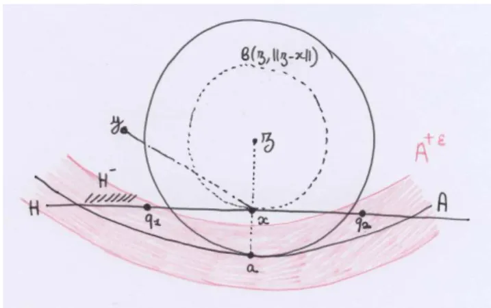
Lemma 14. Consider a subset Q⊂ Aεin RNand suppose
Q can be enclosed in a ball of radius ρ < R− ε. Then, Conv(Q)⊂ Aα for α
Figure 9: Notations for the proof of Lemma 14.
Proof. Suppose R < +∞ for otherwise, A is convex and Conv(Q)⊂ Aε. Let x be a point on Conv(Q) furthest away
from A. By Lemma 13, there exists a point q∈ Q such that kx − qk ≤ ρ. Thus, d(x, A) ≤ kx − qk + d(q, A) ≤ ρ + ε < R, showing that x has a unique projection a onto A. We claim that the plane H passing through x and orthogonal to the segment xa is a supporting plane of the convex hull of Q. To prove this, consider the two open half-spaces that H bounds and let H− be the one half-space that does not contain a.
Furthermore, consider the half-line with origin a that passes through x and let z be the point on this half-line at distance R from a (see Figure 9). By construction, B(z, R) is tangent to A at a and its interior does not intersect A. We prove that Conv(Q)∩ H−=∅. Suppose for a contradiction that
there exists a point y ∈ Conv(Q) ∩ H−. Then, the whole
segment xy belongs to Conv(Q) and in particular intersects B(z,kz − xk). But points in the interior of B(z, kz − xk) are furthest away from A than x, contradicting the definition of x as the point of Conv(Q) furthest away from A. It follows that H is a supporting plane of the convex hull of Q as claimed. Thus, Q∩H is non-empty and can be enclosed in a ball of radius smaller or equal to ρ. The convex hull of Q∩H contains x and by Lemma 13, there exists a point q′∈ Q∩H
such thatkx − q′k ≤ ρ. On the other hand, kz − q′k ≥ R − ε.
It follows that kx − ak = R −pkz − q′k2− kx − q′k2 ≤
α.
Lemma 15. For any subset Q⊂ RN and any convex set
C⊂ RN, Conv(Q + C) = Conv(Q) + C.
The proof is straightforward and hence omitted.
B.
PROOF OF LEMMA 2
We start with a preliminary lemma.
Lemma 16. For all points c1, c2 ∈ C, c1 6= c2 and all
vectors n1∈ N (c1) and n2∈ N (c2), we have
(c1− c2)· (n1− n2)
kc1− c2k2
= 1
2(κc1,n1(c2) + κc2,n2(c1)),
where κx,n(y) is the curvature of the sphere passing through
points x and y and with outer normal n at point x. Proof. See Figure 10, left. Let Sibe the sphere passing
through points c1 and c2 with outer normal ni at ci, for
i∈ {1, 2}. Let n′
2 be the outer unit normal to S1 at c2 and
n′
1be the outer unit normal to S2 at c1. We have
(c1− c2)· (n1− n′2) = κc1,n1(c2)kc1− c2k 2 (c1− c2)· (n′1− n2) = κc2,n2(c1)kc1− c2k 2 (c1− c2)· (n′2+ n1) = 0 (c2− c1)· (n′1+ n2) = 0
Summing up these four equations gives the result.
Figure 10: Notations for the proof of Lemma 16 and Lemma 2.
Proof of Lemma 2. We first prove that for all points c1, c2∈ ∂C with normals n1 and n2 respectively:
(c1− c2)· (n1− n2) ≥ κmin(C)kc1− c2k2.
Consider a sphere S tangent to ∂C at point x and meeting ∂C in another point y6= x. Let D be the ball that S bounds. We begin by proving that κmin(D)≥ κmin(C). Consider a
2-dimensional plane P passing through x and y and containing the common normal to ∂D and ∂C at point x. In particular, P passes through the center of D. We think of ˜D = D∩ P and ˜C = C∩ P as two compact convex sets in R2. By
construction, ∂ ˜D and ∂ ˜C are C2-smooth curves tangent at
point x and meeting at point y6= x. Thus, we reduced the geometric situation in RNto the same situation in R2. Let us prove that κmin( ˜D)≥ κmin( ˜C). Suppose for a contradiction
that κmin( ˜D) < κmin( ˜C). In other words, the curvature
of circle ˜D is smaller than the curvature at any point on the curve ˜C. Theorem 1 in [19] tells us that ˜C, except for x, lies in the interior of ˜D, as illustrated in Figure 10 right. But, this contradicts the fact that ˜C intersects the boundary of ˜D in y 6= x. Thus, κmin( ˜D) ≥ κmin( ˜C) and it follows
that κmin(D) = κmin(D∩ P ) ≥ κmin(C∩ P ) ≥ κmin(C),
as claimed. In other words, given two points x 6= y on the boundary of C and a unit vector n ∈ N (x), we have just proved that the curvature κx,n(y) of the sphere passing
through x and y with outer normal n at point x satisfies κx,n(y)≥ κmin(C). Applying Lemma 16 gives the claimed
inequality.
To prove that the inequality is tight, note that if c2 tends
to c1 along a curve γ in ∂C, then the ratio
(c1− c2)· (n1− n2)
kc1− c2k2
tends to the absolute value of the normal curvature of γ at c1. In particular, if|κN −1(x)| reaches its minimum at x = c1
and the tangent line to γ at c1 is the associated principal