X 'ex R.. Z ... .... A . MIMI. 'n W."
-q
? 1.8 '0 -0 9: Za... '1Z .. .. ... z J .... . .... ... . .. . .. .... ... .... .. 41-yr. Or N v 0" .... ... A A A u I.X J, z A ? 'e. A T, ov 41MITLibraries
http://libraries.mit.edu/askDISCLAIMER NOTICE
MISSING PAGE(S)
IN COMPEESSORS AND TURBINES
by
EIJI YOKOYAMA
Under the Sponsorship Of General Electric Company Westinghouse Electric Company
G&s Turbine Laboratory Report Number 63
Massachusetts Institute of Technology
Acknowledgement Abstract
List of Symbols
1. Introduction 1
2. Description of Test Apparatus
3
2.1 Low Speed Wind Tunnel Cascade
3
2.2 Probes 4
3. Test Results 4
4. Discussion of Test Results 5
5. Modified Lifting-Line Theory 8
5.1 Single Flat Plate Wing 8
5.2 Tip Clearance Effect 14
6. Conclusion 18
Appendix I Evaluation of Static Pressure on Suction Surface 19 Appendix II Circulation Around Two-Dimensional Airfoil 26
The author wishes to express his sincere thanks to Professor
E. S. Taylor, Director of the Gas Turbine Laboratory, thesis
supervisor, for his generous help and many suggestions; to
Professor Y. Senoo for his kind guidance as the supervisor until his departure; to Professor P. G. Hill for his valuable suggestions; to Mr. M. Lefcort for his help in the flow observation study and many suggestions; to Mr. Dalton Baugh, Mr. Basil Kean and other members of the Gas Turbine Laboratory for their help in making probes and arranging the test apparatus; and to Mrs. Elizabeth Johnson for typing this report.
The influence of tip clearance on the lift distribution along a blade span was studied on linear compressor and turbine cascades. The wall boundary layer was removed by means of the intage technique. The lift distribution in the span direction was found to be almost
similar for both compressor and turbine cascades having the similar velocity diagrams. The lift acting on the blades increases toward the blade tip. The phenomena were explained theoretically by con-sidering the velocity induced by tip vortices on the blade surface.
A aspect ratio
a radius, inches
b span, inches
Cl section lift coefficient
Cn section normal-force coefficient
CN normal-force coefficient of isolated airfoil
Cp pressure coefficient ' Cyp
Cx2 inlet axial velocity, feet per second
C
2outlet axial velocity, feet per second,
c blade chord, inches F complex potential
PO stagnation pressure, pounds per square foot
p pressure on blade surface, pounds per square foot
p1 upstream pressure, pounds per square foot
R distance between point on surface and tip vortex line, inches
Re Reynolds number
r distance between point on surface and tip vortex segment, inches
s distance from leading edge along tip vortex line, inches
u velocity in 'chord direction, feet per second.
V inlet velocity, feet per second
V outlet velocity, feet per second 2
V2d velocity around two-dimensional airfoil, feet per second v velocity in span direction, feet per second
w velocity normal to blade surface, feet per second
w velocity w induced by tip vortices, feet per second
x chordwise distance, inches
Y non- dimensional spanwise distance y/c
y spanwise distance, inches
YO clearance to chord ratio, y /c yO tip clearance, inches
Z complex plane
z distance normal to blade surface, inches
o( local incidence angle, degrees o(., incidence angle, degrees
outlet angle, degrees
o(qo mean flow angle, degrees
( angle between blade surface and tip vortex line, degrees
T circulation of bound vortex total circulation around profile
non-dimensional circulation around profile
F
circulation of tip vortexF~
non-dimensional circulation of tip vortex circulation around two-dimensional airfoil Fbuxrier coefficientcompalex plane
spanwiise distance, inches stagger angle, degrees chordwise distance, inches
It is well known that the amount of tip clearance haG a large effect on the performance of axial flow machines. The results obtained by past
(1) experiments show different trend from compressor to compressor and it seems to be difficult to obtain a generalized expression for the effect of tip clearance.
The flow phenomenon in the vicinity of a blade tip in an axial flow machine may be considered as a combination or an interaction of phenomena due to three different causes, i.e., the amount of tip clearance, the boundary layer on the annulus wall and the relative blad.e tip velocity to the wall. To
study the problem in detail, an experiment was conducted by G. Khabbaz(2) in the Gas Turbine Laboratory in 1959. In this experiment, the tip clearance effect on stall limit of compressor cascades was studied using the image method to eliminate the wall boundary layer. He found through the test that
1) stall occurred at a higher angle of attack near the wing tip than
for the remainder of the blade,
2) as the clearance size is increased, the loading on the blade near the tip increases, while at a greater distance from the tip it remains unchanged.
He explained the pl nomena by applying the momentum theory to a control volume taken between the blade tips as shown in the figure.
net momentum flux out = (p1 - p2) x Area
For compressor cascades, the pressure at the outlet of
-~ -- the blade row p is higher than
CON T OL the inlet pressure pl, and the
Vo LumeS
control volume must be larger than that going out from it. Accordingly, some air must leave the cascade by passing through the blade row to
satisfy the continuity. Since the flow at a greater distance from the tip is two-dimensional, this flow will increase the local velocity near the tip and result in an increase of the lift near the blade tip.
If this hypothesis is correct, then the reverse result must be obtained for turbine cascades because the pressure at the inlet of the turbine cascade is higher than that at the exit.
The experiment was continued by the authro to check this effect. After the cascade test, it was thought that it was necessary to observe the flow near the tip for understanding the phenomena in more detail, and flow observation was attempted by using tufts in the cascade and
by the ink tracing method in a water table.
2.1 Low Speed Wind Tunnel Cascade
The experiments were carried on the same apparatus used by G. Khabbaz. The cascade consists of nine blades; four of them were cut in halves to make the clearance (Fig. 1).
The dimensions of the cascade are given in Table 1.
Table 1 Blade Profile
Chord Length Solidity
Clearance to Chord Ratio
Stagger Angle Air Inlet Angle Air Inlet Velocity Reynolds Number*
Dimensions of the cascade
NACA
65-410
C
= 4.875
in.
c' = 1.0y=
yO/c = .03 Compressor550
D=65*
V 110 Ft/Sec S e= 2.8 x 10⁵ Turbine 50=
54* = 70 Ft/Sec = 1.8 x 10⁵(*) Based on inlet velocity and chord length
The blade surface pressure was measured by two blades in the middle of the cascade. The pressure taps on these bibades are located along the chord at various distances from the blade tip as shown in Table 2. Static pressures were fed into a multi-tube inclined manometer by vinyl tubes.
Table 2 Position of Static Pressure Taps on Blade Surface
Chordwise Distance from Leading Edge (percent chord)
No.
1
2
3
4
5
6
7
8
9
10
1
12 13
14
15
Distance 2.5 5.0 7.5 10 20 30 40 50 60 70 75 80 85 90 95
Spanwise Distance from Blade Tip, inches
No.
1
2
3
4
5
6
7
8
Distance
1/16 3/16
7/16
11/16 15/16
1 /16 2 /16
4 /16
2.2 Probes
A pitot static tube was placed at a chord length upstream of the
blade row for measuring the inlet velocity and pressure. The flow down-stream of the blade row was measured by traversing a five-hole probe in a plAne at a chord length downstream of trailing edges of the blades. The pressure tubes frm the probe were connected to a wirestrain gauge type transducer and the pressures were read by a D.C. balancing bridge type calibrator.
3 Test Results
Fig. 2 shows the pressure distribution on the blade surface of the compressor cascade. It can be seen from the figure that the static pres-sure on the suction surface decreases considerably as the blade tip is approached, but there is little change in pressure on the pressure surface.
The static pressure on the suction surface at different chords were plotted against the distance from the blade tip in Fig. 3. The region influenced due to the tip clearance is spread toward the trail-ing edge along the chord except in the vicinity of the leading edge.
The outlet axial velocity obtained by the wake traverse was divided by inlet axial velocity and plotted in Fig. 4. It shows a typical wake
shape at y/c = 0.4, but for smaller values of y/c, the pattern deforms gradually and a highest velocity appears at downstream of the suction
side and lowest velocity at downstream of the pressure side of the blade.
Fig. 5 shows the distributions of the mean axial velocity, the turning angle and the lift coefficient along the span. The mean value of the outlet axial velocity and the lift coefficient were obtained by integrating curves in Fig. 4 and Fig. 2 respectively. The turning angle was calculated by using continuity and momentum equations assuming that no mixing occurrs in the spanwise direction. The outlet axial velocity and the turning angle decrease toward the tip in spite of the increase in the lift coefficient.
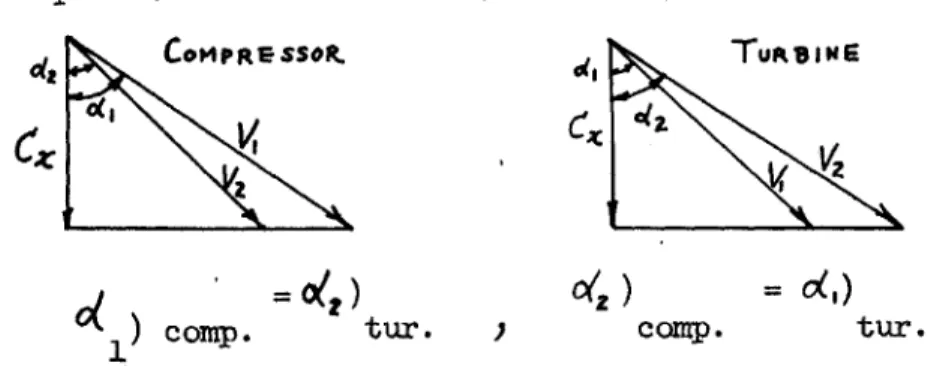
Surface pressure measurements wore also made for a turbine cascade. The stagger angle in this case was so chosen that the velocity diagrams for compressor and turbine cascades are similar.
COMPRESSOR. TuUijE
c4)
.) = d,))
comp. tur. .i coMp. tur.The surface pressure distribution is shown in Fig.
6,
and thenon-dimensional lift coefficient is plotted in Fig. 7 together with the results obtained from the compressor cascade. The trend is almost the same for both cascades.
4 Discussion of Test Results
The test results may be summarized as follows:
axial velocity decrease near the blade tip in spite of the increase in the lift coefficient.
(2) For both compressor and turbine cascades, the lift coefficient increases toward the tip.
These phenomena cannot be explained by the momentum theory which was applied to this problem by Khabbaz.
Before entering the discussion of the tip clearance effect, let us look at the flow around a single wing of finite aspect ratio. There are some reports concerning the lift or pressure distribution along the span of wings of small aspect ratio. Fig. 8 is one of the test results obtained by Holme. The lifting surface theory shows the
correct behavior for very small angles of incidence. However, as the angle of attack is increased, the loading becomes larger near the tip. Except at small angles, the lifting surface theory gives very
inaccurate results even for angles of attack much smaller than the stalling angle.
To investigate the flow phenomena near a wing tip in detail,, flow was observed by tufts in the wind tunnel and also by the ink tracing method in a water table. In the experiments, a strong wing tip vortex was observed as shown in Fig. 9. Air rolls up around the wing tip and makes a wing tip vortex above the suction surface. This tip vortex will have a large influence on the blade surface
pres-sure, especially on the suction surface since the vortices exist above the suction surface. To confirm the effect of tip vortices on the surface pressure, a crude calculation was attempted under the fol-lowing assumptions.
1. Velocity on the blade surface is approximately the sum of
the effect of trailing vortices are neglected since the strength of trailing vortices were observed to be much smaller than that of the tip vortices.
2. The distribution of the bound vortices along a chord is approximated by a linear function of x/c, because the circulation of a bound vortex is proportional to the pressure difference between the
surfaces, and the pressure difference would be approximated by a triangle as shown in the figure.
ACTUAL 'PRESSU*E
---
ArPOXMAT
ED 0Figure 1O
0
I.0
5.
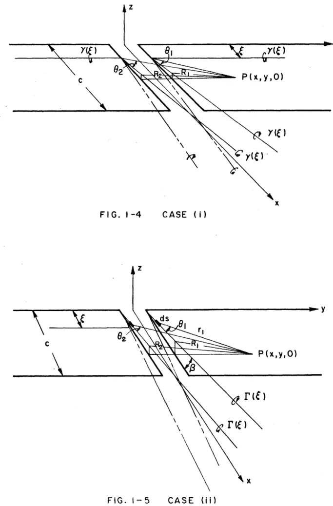
The tip vortices are a continuation of the bound vortices and exist in the x-z plane (Fig. i-5) with an angle P to the x-y plane.Two different assumptions were made to express the position of the tip vortices.
i) The wing tip vortices leave from the wing tip parallel to each other. (Fig. I-5-i)
ii) The wing tip vortices leave from the wing tip and join a vortex which started from the leading edge with an angle to the blade surface. (Fig. I-3-ii)
In both cases, the angle 0 was approximated as equal to the angle between the chord line and mean flow direction, that is
The pressure on the suction surface at y/c = .0385 was evaluated
by taking images of the tip vortices to satisfy the boundary co. lition
on the surface (see Appendix I). Vz = 0, on surface (xy,O)
The result was plotted in Fig. 11. The pressure distribution along the span was also calculated at x/c = 0.5, and shown in Fig. 12. The pressure distribution calculated by the assumption (3-ii) shows com-paratively good agreement with the test result. We will be able to say from the figures that the assumptions made for the calculation are not far from the actual flow phenomena. However, the procedure used here, i.e. the use of the image vortices to satisfy the boundary condition is not applicable in evaluating pressures on the pressure surface.
(7)
In the lifting surface theory, this boundary condition was satisfied by the relation
w + V1 Sin 0l = 0. (1)
That is, the normal component of the induced velocity cancels the normal component of inlet flow.
The problem may be solved by using Eq. 1 as' the boundary con-dition and the calculation procedure will be similar to that for the lifting surface theory, the only difference is that the equation would involve additional terms due to the tip vortices which were not considered in the original lifting surface theory.
The treatment of the problem as a lifting surface will be much more complicated and a laborious numerical calculation will be
required to solve it. If our main interest is to know the distribu-tion of lift in the span direction, this complication may be avoided
by means of the lifting line approximation. The procedure will be
shown in the following chapter.
5 Modified Lifting-Line Theory
Z
.2
Figure 13
Consider a flat rectangular wing placed in a free stream of
velocity V1 with a small angle of attack 0( . Some air flows from the bottome to the top around the wing tips due to the pressure dif-ference between the surfaces, and trailing vortices are formed from
(6)
the trailing edge of the wing a. explained by Prandtl. However, as the angle of attack 0( 1 is increased, the pressure difference
between the surface increases, consequently a strong upward flow
appears around the tips, which rolls up above the suction surface
and forms wing tip vortices as shown in Fig. 14. The wing tip vortices
-Z
z
induce velocity in the direction from the center of the span to the wing tips, the magnitude of which is approximately inversely proportional to the distance between the vortex and the point on the surface and propor-tional to the cosine of the angle 9 shown in Figure 15.
z
J2
Figure 15
The interesting thing is that the direction of this induced velocity is opposite to that in the Prandtl hypothesis.
In the Prandtl theory, the trailing vortices were considered as the continuation of the bound vortices and the system was replaced
by a set of horseshoe vortices (fig. 16). If the same assumption is
made for the present case, i.e. the wing tip vortices and the trailing vortices are considered as the continuation of the bound vortices, then the system will be as shown in Fig. 17.
I
Figure It can the profile value which _ 9I
-p - --16 Prandtl's Hypothesis Figure 17 Present Case be seen from Fig. 17 that the total circulation [j)around increases toward the tip and at the tip it has a finite is equal to the circulation of the wing tip vortices
FO.
Lifting Line Approximation
For the wing of large aspect ratio, A = b/c 9 1, the system in Fig. 17 may be simplified to the system shown in Fig. 18; the wing is replaced by a vortex of circulation
r(|)which
is an unknown function of y.Figure 18
The induced velocity at a point P(O0,y) is the sum of velocities induced by the tip vortices and the trailing vortices, since a bound
vortex induces no velocity at its own center.
.Applying Biot-Savart's law (Eq. I1-4) to the system, the velocity
induced by the tip vortices which extend from x = 0 to x = o is given
by
'The negative sign in the equation means that the induced velocity is in the negative z-direction.
.r
The velocity induced by a trailing vortex of circulation LjIthrough the point Q (0,Fj ) is
4. 4 7 --
()-3)
Integrating Eq. valong the span, we get the induced velocity due to
all the trailing vortices
by
thepoi tQt
CO"')id
X(f b4
z'l~
Thus, tile total induced velocity at P (0, r= ,+ Wtr r~~)~ Y) becomes3
o
7L1
I
~
O __ __ (5) zXThe total circulation around the profile is expressed as (see Appendix II)
~
)
-.
cW s.
=c
/1st(,
+
)
.
(6)
For a small angle of attack, Sin ot'N 0(, , then
Uw)
=7cV(d,+
)
=
7c
c
1+i +
- ca
+
(7)
Substituting Eq. 4 into Eq. 7, we obtain
66
Fm
,cVd.
- cFofdoT
~
I.
The first term of the equation is equivalent to the circulation
(8)
of a two-dimensional wing, that is the circulation around a wing of infinite aspect ratio, so we definevz2
==
77:C V (,
(
9)Dividing Eq. 8 by Eq. 9, we get
EM
T
(+)._.
+
d
d.
whereT
(10)
FV)
The variables y and I may be changed into 6 and
f
by the followingrelations - Cos S= - CWs4' C
A
(-
Cos&)
==
-(9)
.
(11)
() I-Cos 2 Ces
#
-- Ce 6S-o
where A aspect ratio = b/c.
Assume
F()
may be represented by the function[~() =
o+
z F, si-n?L.
e
since (6)has a finite value at G = 0 and 9=
Noting that n must be an odd integer to ensure the equality Sin nG = Sin n (1( -6),
n is taken as
n = 2m + 1, m = 0,1,2, , . ..
Substituting Eqs. 13 and 14 into Eq. 12, we get
a t
0
r~Et'r
= I - iC, 5 9 (15) _ _- Co,(zm+,)+df
2A
focos
+- Cos6'
Evaluating the integral on the right hand side and noting that
e = > must be omitted since a vortex induces no velocity at its own center,
it
Cos
(2M+)
S CO.s - Cos 0
CCs (2M+I)+ d
Cos+
-Cos
e
p
Q+ETherefore, it follows that
(
0-5Cos20 or bn*111o
+
Zo
",MO...
+.)
[+-A
2A
I \+ C0.5 9+ -
zmi+I
Ln (zMP+0
ZA
s'ff
0
(16) -(12)("5)
(l4) the point"'+"
S,'. (2m+ )e s4A (z ? + 1) IE
0E
&n (2 rn +Q i =z n76 + I \C sby taking a finite number of particular values of 9 . For &= 0,
the term l/(1-Cos e ) in Eq. 16 must be set equal to zero for the same
reason described in evaluating theintegral of Eq. 15.
The theory developed above will be useful for evaluating the lift distribution along the span for wings of large aspect ratio, since the theory was derived based on the lifting line approximation.
As an example, the distribution of normal-force coefficient
for a wing of aspect ratio 6 was calculated by locating 9 at 0, 30, 60,
and 90 degrees.
The normal-force coefficient Cn was divided by the mean value of
Cn, that is b
and the result was plotted in Fig. 19. The curve shows the correct trend at the region near the wing tip.
.2 ij Clearance Effect
G.
r.
Figure 20
Place three blades in a plane with clearances 2yo between the adjacent blades.*
_ 1. First an attempt was made to solve the problem for two blades of semi-infinite span. However, the solution was found to diverge since the wing span extended to infinity. 'his trouble may be avoided by
The induced velocity at a point P (0,y) can be evaluated by the same manner as in the previous calculation.
Velocity induced by tip vortices;
I 1 +
1
I+ b-+ t . -- b + -y6 I~o1*
(I)~
-0 i ('.+6
2 j" (,+f-y ( 2 -L (z I' +4
____t_+Velocity induced by trailing vortices;
r
rr
Substituting Eqs. 17 and 18 into Eq. 7, we get the expression for
the distribution of circulation along the span.
+
b
2 +Y2 I4
-I+ I _ _ _ _ T 19
zI
Changing the variables by the relations
U=
.s
C
,
= - - Costand using the non-dimensional expressions
rw
4
Fo
[/O(20)
solving the problem for long blades but finite span.
2. Three blades were taken instead of two, so that the lif.; dis-tribution along the span can be considered as symmetric to x axis and the calculation would be much simplified.
*X
('*)
b Eg. 19 becoFte)
-(--kCase)
A
_-Acs6
mes as follows: - ' -a0
.3 +
4
Y/,,
(3+4YI- Cos' 6
('
+
4
V4 , 4 )2_ C,,20o s L - Coso (2+4 (as )+Cos .
Again
ri9)is
assumed asM=o (2(+2 / and then, / 00
r
(41)
= z "su 0(z*n+e)
+ Cos (z n-+) +O
t(24)
From Eq. 22, 23 and 24, we get-m1o:-r
s0
(zm-
1)A L -Cos
~~ "CO +1+ 3 t+4 A
s
(s 4
z) -cS'
-I-12,
S+ 4 YYA
0+4
)
1-CosO]
,,,
.
3
j
-CCs
( m +i)+
Cos'1'
Cs9
0f:
K
f+ Cos+
O 3, - Cos t XSin
(zmi+1)e
S-L ) (21) (23) whereI
(25) d+.(22) (2+4 ,4+C49)-K,=
2 +4
f
-Cos
0
>I
K,
==+4
Cos0*
- i or O~g9 !C 7
The solution of integrals I2,, and l cannot be expressed in simple forms like that of I,m. iere, the integrals were evaluated step by step and the following equation was obtained:
-=4+.
+
3 + 4
i -4(3++)-Cos 2O (1+4 4)-CosG)4
-
S+
[3
K,
KI
2,4
1/ ." -I I -- 33 zK, (4
-4-3)K
z(4 Ka--3)
z r3+ .Z2A-
+
++4(K, -+
Kz)-)
l e ,K| -k-+
7E
+ (6(K
k4'4
K.)-2(K,
)
+2K, ( 1
6K, -20K, 2+ 5)
xz (16
4 ,-2OKz+-5)
+ -- - - -(26)
The equation may be useful for wings of large aspect ratio and with comparatively large tip clearance. A numerical calculation was
tried for A = 10 and Yo = 0.1, and the result war; compared in Fig. 21 with the test result obtained by Khabbaz.
It can be concluded from the results obtained by the cascade tests that:
1) For a compressor cascade, the lift coefficient increases near the
blade tip in spite of the decrease in the turning angle and the outlet axial velocity.
2) For the turbine cascade, the lift distribution in the spanwise
direction shows a trend similar to that for the compressor cascade.
The problem was approached theoretically by considering a simpli-fied vortex system, and the pressure distribution on the suction sur-face was calculated from the induced velocity due to the tip vortices. It shows a fairly good agreement with the test result.
Appendix I Evaluation of Static Pressure on Suction Surface
(1) Biot-Savart's Law
Figure I-1
If a vortex filament of circulation
F
lies in a plane, the velocity induced at point P(x,y) by the vortex segment (y Y Y 2 can be evaluated by the law of Biot-Savart.I-. t
(I-i)
4
r
Considering the angle
e
as the variable, we have1 - =X Cot 0
,
d
and (1-2)
Thus,
T
r ==n
--0,:.
dO
(COS
19Z
Cos
01
),
If the vortex filament extends to y + oo , then
n=
, Cosez
= -1, and the above expression becomesF
=(I
+Cos
).
(1-4)
(2) Circulation of Bound Vortex Z
C
Figure (1-2)
According to the assumption (2) on page 7 , the circulation of a bound vortex at x = { would be expressed as
Integrating this equation along the chord, we obtain the total circula-tion around the profile.
c
C*j
(I-5)
or
ZrV
o
C
where
F
is the circulation around a two-dimensional wing accord-ing to the assumption (1) on page 6Substituting Eq.
1-5
into Eq.1-4,
we get(3)
Induced Velocity at P(x,y,o)To satisfy the boundary condition on the surface, that is
w = 0, on P (x,y,0)
Case (i)
The velocity at point P(x,y,o), induced by the tip vortices which leave from the wing tips at x = is expressed as (see Fig.
-(x-) 0 )
+
c.,
e,
2 X. R,1+
Co's
jZ
Ia
(I-7)
2 =(
RI
(~)SQ
+
-t)
t + Y"2Ces
9, =(
X-
)
(OSP
&
-
k(x
+Co
,Ccs Oz
vC.
(x-)z + ('I+ f
(I-9)
Substituting Eqs. 1-6, 1-8 and 1-9 into Eq. I-7, we obtain the
equation for the induced velocity.
-1v
~J.(x-k)(c-g)S..t
{-g
Z(1-).+
tC
Q +
Ea . Cz h e t in pfrtial +f(i
-Sx +(I + +x1Co
Expanding the equation in partial fractions., we get
.
S
.
k V t.2rt'
(x-k)cos
*O)gI
CJ
C (x - l)(c -- ) z ___(__-__(c - _(z-jk/
S4&9
+(1 -)
f(x- g)*
ZSZ9(+
#0 C os(- ?+
(c -.-+
s
-o
6)L
Cos- ) Ii +( y+.)(-o + CIL6-.
where
I-4)
(1-8)
-The integrations of Eq. I 10 were evaluated term by term and the
following result was obtained.
- x - X-K SltP + (Y + Y )
X,
Si- +(YY.2
_X)2 S
(
(-XY(s
+
Y
(,+
x
cos
()[,
-
x
Cos
,+
-x)c.sf44--()C)
J
Y- YY
+ YY-YO
-x ef Y+n OY-
Ye
Y+YO.Y - ,
YO
Y
-Yo
Y+f Y-Y. sj; Y+ yo[*, +X2( I(
-x4
-2,
t
Cos
I(I-11)
Whe re. VU - A T-y-e-xY
-(Y+YVZ
(I-iz)
-x -+Y1YO
;
- 7Lc sinU-z c
4-ZCase (1
From the geometry in Fig. 1-5 and Biot--&"avert'
;
law, the velocity induced at point P(x,y,O) by a vortex segment ds is formulated asf ollows:
F.Msi.6ids
x
sk
2a
R~~YZ)
2
ie
G
(m
X S,--n
X -~()xSat ?; Circulation of the tip vortices ()May be written as=fFc
CzF(C~
J
fJ
Fa
fo) rt*~
)M d= = =
z
dfor
(
>
c
)
h
r , r2 and ds are expressed. in term (' I, a rnd JL as follows.
xR- 15) (I-14)
Cos
P
=
I
Cos 9 Y= R R1 + (( Cos - Sec Y YZ == z + (X Cos(3 -- ISec.)Substituting Eq. 1-14 and Eq. I- 15 into Eq. 1-13, we get
C
. C e ( (X C-s
-Se
.j (Cose- 5&cJ+~ f (Cf 1_________ I
(I-16)
Integrating this and rcarrzuging, we obtain the equation for the induced velocity at point P(x,y,O).
z 7E C V X [-; S(4 rCs'f
3R'
2+(K
Cs -Sec ) (xCos
SeCq) R, z C 2R
(kcoses
ec) tSw'
)
+
(zS
,
-XC.s)
I
+
Sec,
2 e I -(X Cos P -Sece) + /(X ce(x
Cos - Sec t) +/(X Cos4 , -t caj X CO3S tz x Cos
-
+t
X2
S .-n a + Y-x 1,sc-( +(Y.' t y.I
The pressure coefficient on the blade surface was calculated as follows.
According to the assumption 1 in P. 6 , velocity on the blade
surface is expressed as
V7
=
V
2
Z +v
z 1~I,I
w h re
(1-17)
(1-18)
where V2d : velocity vector on a two-dimensional blade surface,
9; : velocity vector, induced by the tip vortices.
The magnitude of the velocity is
V V2 + 2
or
V2 V2d + V2 (1-19)
Bernoulli' s equation for two-dimensional flow;
P p1 + (1/2)V 2 p2d+ ( f/2)V2d
or
(p- = ( F/2) (V -
V
2d ' For three-dimensional cases, it becomesp - p = (f/2)(V 2
v
2) = (/2)(V 2 2) - (Sf/2)v2= (P - p1)2d - (J/2)v
2
Dividing this equation by inlet dynamic pressure, we get the expres-sion for the pressure coefficient.
z(1-20)
As an example, the pressure coefficients were calculated for the tested compressor blading using Eqs. 1-20, 1 -11 and 1-17. The results
Appendix II Circulation Around a Two-Dimensional Airfoil
The circulation around a wing of infinite aspect ratio can be obtained
by means of the conformal mapping.
z - t?
a--za-2(..
A circle of radius a given on the Z-plane is mapped into a straight
line (-2a ! t 1 +2a) in the -plane by the function
z
The complex potential of flow around the circle in the Z-plane is expressed as
F(Z)
V
e-
Z
+
V
e
,
+
i
z
Differentiating this equation with respect to Z, we getLF
-,;.,
Ve
A
a
2F_
2 z TL Z
The circulationF can be found from Eq. 11-3 with the boundary condition
=
0
SJZ
af
z
=a2
(11-4)
Thus,(11-5)
.(1-2) (11-3) -a \(II-1)
4 -i
aV, S
,,.
oe,
=
7E c
V/,s,,t
a,6
REFERENCES
1. McNair, R. E., "Tip Clearance Effects on Stalling Pressure Rise in
Axial Flow Compressors" Westinghouse Electric Corporation, Lester Plant Steam Division Engineering Report E-1389, March, 1960.
2. Khabbaz, G. R., "The Influence of Tip Clearance on Stall Limits of a Rectilinear Cascade of Compressor Blades" Gas Turbine Laboratory Report No. 54, M.I.T., August 1959.
3.
Winter, H., "Flow Phenomena on Plates and Airfoils of Short Span"NACA T.M. No. 798.
4. Holme, O.A.M., "Measurement of the Pressure Distribution on Rectangular Wings of Different Aspect Ratio" Flygtekniska Forsosanstalten, FFA No. 37, 1950.
5. Milne-Tomson, L.M., "Theoretical Aerodynamics", 3rd ed., p. 80, Macmillan and Co. Ltd., 1958.
6. Glauert, H., "The Elements of Airfoil and Airscrew Theory",
Cambridge University Press, 1959.
7.
Blenk, H., "Dew Eindecker als tragende Wirbelflache", Z.a.M.M.,Vol. 5, p. 36,
1925.
CTION SLOTS
BO UNDARY
LAYER SUCTION
(POROUS
WALL)
KJKNJKJ
PRESSURE TAPS
ON SUCTION-SIDE
\PRESSURE
TAPS
ON PRESSURE -SIDE
FIG. I LOW SPEED CASCADE
SU
I
0,2
0
swm a m* i0 -+
-w -m-- --- J---0.4
x /cDISTRIBUTION
Y -o
c c -Y -Yo Sc 0Y -Yo
C=.0898
.141
.192
=.346
y -yo-5E55
c,= T WO-DIMENSIONAL
0.6
0.8
ON BLADE SURFACE
Iso
OF
A COMPRESSOR CASCADE
X--X-X-X.X'DISTANCE
FROM
TIP
*_----
_--
.0128
---
X----
-
=.0385
c
-0.2
-0.4
-0.6
-0.8
0
0.2
FIG.
2 PRESSURE
I
p
v,2
0.4
0.2
0
p -p
1}P
V2-0.2
-0.4
-0.6
...--
-
-
--
x/c
=0.9
x/c
=0.7
+-A
-x
- - - - -x - ..
0
0.1
0.2
0.3
y -
Yo
C
x/c=
0.5
-mx
x/c = 0.3
x/c =
0.1
0.4
0.5
0.6
FIG. 3 BLADE SURFACE PRESSURE AT VARIOUS CHORDWISE
VS. DISTANCE
FROM TIP
DISTANCES
I
I
I
I
I
I
I
----
- -- -- --Of
%.
+ oool
PRESSURE SIDE
T
SUCTION
DISTANCE
FROM CENTER
OF CLEARANCE
y/c
=
.402
x
- ----+
y
y/
c=.197
y/c
= .145
y/c
y/c
y/c
=
.0941
= .0685
=
.030
0.4
DISTANCE
0.6
ALONG BLADE
BLADE SPACING
FIG.4 DISTRIBUTION OF
FOR COMPRESSOR
OUTLET AXIAL VELOCITY
CASCADE
0.8
I-C0
20.7
SIDE
0.6
[--0.5
0.4
0
0.2
0.8
1.0
ROW
I
I
I
I
II
-
1.0-
0.8-10-I
0.6-
9-
8-
7-
6-a
1
-c
2
(deg.)
oX
XaumXCx
2/Cxl
w
z
c
wl
-J w-Yo~ 04'C'2
x
0
0.1
0
TIP
0.1
0.2
DISTANCE
i
0.2
0.3
DISTANCE
FROM CENTER OF CLEARANCE
FIG. 5 DISTRIBUTIONS OF LIFT COEFFICIENT, OUTLET AXIAL VELOCITY AND TURNING
ANGLE VS. SPANWISE DISTANCE
C/C4 2 d
_v
X
X.00
X.--w
A0.3
FROM
TIP
0.5
0. 4 Y
c
0.6
i
0.4
0.5
i
0.6
i
y / c
0
0.7
I
I
I
DISTANCE
FROM TIP
y~Y
=(12R
c
-- mX--Y
=.0385
Y
-Yo
.0898-4
-y14
Y Yo
346
TWO-DIMENSIONAL
4---6.
-U.n
I-x..
IIaool
.mo
0
0.2
0.4
x/c0.6
0.8
FIG.6 PRESSURE
DISTRIBUTION
ON BLADE
SURFACE
TURBINE
0.5
0
p-p2 IpV
2 --- I-1.0
-1.5
-2.0
1.0
OF
CASCADE
I
-.-
o --.
/X
C
-- X-- T~XT
x
x
)MPRESSOR CASCADE
JRBINE CASCADE
0>--
--0.2
0.3
DISTANCE FROM
0.4
Y
-Yo
TIP
FIG. 7 COMPARISON OF
CASCADES
LIFT DISTRIBUTION
FOR TURBINE
AND COMPRESSOR
1.15
1.10
C
/C2
zd
1.05
1.00
0.95
0
0.1
0.5
0.6
I
I
I
I
I
I
1.2
IgoCn/CN 0.8
ASPECT RATIO
=1.0
al
a I
0.6
-0-O-
4
--
X- 160
0.4
_ --
8*0
-
-
20*0
-
2*
-
LINEARIZED
LIFTING SURFACE
0.2 ~
THEORY
0
0.2
0.4
0.6
0.8
1.0
CENTER
(b/2)
TIP
EXPERIMENTAL
FIG.8 NORMAL FORCE DISTRIBUTION ALONG SPAN OF
RECTANGULAR WING OBTAINED BY HOLME
SUCTION
SIDE
LEADING' EDGE
(j)m
H C) I 0 ~1z
H -Q 0 Hm
TRAILING
ED-GE
IF
MITLibraries
http://libraries.mit.edu/askDISCLAIMER NOTICE
MISSING PAGE(S)
CLEARANCE TO CHORD RATIO
yo/c =
.03
DISTANCE
FROM TIP-
y
/c=.0385
/X
I
0
--P
-P1
2
1V
-0.2
-0.4
-0.6
-0.8
0
/L
---x
-
7
"A
o.-'
MEASURED, TWO-DIMENSIONAL
CASCADE
-
X-
MEASURED
--- *---
CALCULATED, CASE
(i)
CALCULATED, CASE
(ii)
0.2
0.4
x
/c
0.6
0.8
FIG.11 PRESSURE
DISTRIBUTION
ON SUCTON
0.4
0.
2
1--//
*eolg1.0
I
I
-- -I
L
-I
SURFACE
-0.2
-0.4
P-pj
pV
-0.6
-0.8
-1.0
--a
ME
CA
----
CA
0
0.1I
SE
SE
0.2
DISTANCE
FIG. 12 PRESSURE
DISTRIBUTION
FROM TIP
y/C
ALONG
SPAN ON SUCTION
SURFACE
AT x
/~c
=
0.5
ASURED
(i
(ii)
0.3
I
0.4
I
0.5
0.6
I
I
.I
I
I
I
MITLibraries
http://libraries.mit.edu/askDISCLAIMER NOTICE
MISSING PAGE(S)
ASPECT RATIO
=6
0.2
0.4
y
(b/2)
0.6
FIG. 19
CALCULATED
ALONG SPAN
NORMAL -FORCE
DISTRIBUTION
OF
A RECTANGULAR
WING
1.6
1.4
1.2
1.0
Cn /CN
0.8
--0.6
0.4
0.2-0
CENTER
0.8
1.0
TIP
I
I
I
I
MITLibraries
http://libraries.mit.edu/askDISCLAIMER NOTICE
MISSING PAGE(S)
yo/C
=
0.1
2.0
CALCULATED
-X-
MEASURED
BY KHABBAZ
X/C2zd
1.0
0
I
2
3
5
DISTANCE
FROM TIP
c
FIG. 21
DISTRIBUTION OF LIFE COEFFICIENT FOR
A COMPRESSOR CASCADE
WITH
TIP
'I I
FIG. 1-3
t
z
ifz
x
Fo
x
ro
0
z
I
v
VI
a,
Cx,
V,
mages
.1y
y
2
P
,,0)
Y