A comparison of solutions of Kepler's and Lambert's problems,

A COMPARISON OF SOLUTIONS OF KEPLER'S AND LAMBERT'S PROBLEMS

by

Louis Anthony D'Amario

S. B., Rensselaer Polytechnic Institute (1968)

Stephen Patrick Synnott

S. B., Rensselaer Polytechnic Institute (1968)

SUBMITTED IN PARTIAL FULFILLMENT OF THE REQUIREMENTS FOR THE

DEGREE OF MASTER OF SCIENCE at the

MASSACHUSETTS INSTITUTE OF TECHNOLOGY (November, 1969)

Signature of AuthorsG _

Copatment of Ael6naitics and Astronautics, November, 1969 i Certified by Accepted by Thesis Supervisor Chairman, Departmental Graduate Committee 1 Archives I I I J _

tAR _{I, .}

K-0

and~~~~~~~~~~~~~~~~~~~~~~~~~~~~

,2P

I.-A COMPI.-ARISON OF SOLUTIONS OF KEPLER'S AND LAMBERT'S PROBLEMS

by

Louis A. D'Amario Stephen P. Synnott

Submitted to 'the Department of Aeronautics and Astronautics on November 14, 1969 in partial fulfillment of the requirements for the degree of Master of Science.

ABSTRACT

Four solutions of Kepler's initial value problem and three solutions of Lambert's boundary value problem are investigated. All the solutions are characterized by the fact that they are universal, that is, applicable without change to elliptic, parabolic, and hyperbolic

trajectories.

The basis of investigation consisted of comparing the accuracy achieved and the computational effort required by each solution under

several different conditions. Two different iteration methods were

studied and the convergence criteria on the iterations were varied. There appeared to be no clear cut superiority of one method of solution of either problem over any other solution. All methods

exhibited both advantages and disadvantages. The major result of this investigation was the demonstration of the superiority of a Newton

iteration scheme over a regula falsi (or linear inverse interpolation)

method.

Thesis Supervisor: Dr. Richard H. Battin Title: Associate Director

ACKNOWLEDGEMENT

The authors are first of all indebted to the Instrumentation Laboratory of MIT under the direction of Dr. C. Stark Draper for

providing the facilities and support so necessary for this work.

Special thanks are due to Dr. Richard H. Battin, our thesis supervisor, at whose suggestion the study was undertaken, and whose advice and comments contributed greatly to the result. We

also wish to acknowledge the considerable assistance of Mr. William Robertson of the MIT/IL whose encouragement and helpful suggestions were so important during the work and in writing the results.

The typing of the thesis was undertaken by Mrs. Anita

Tucholke and Mrs. Susan MacDougall. Their effort and perserverance

are greatly appreciated.

This report was prepared under DSR Project 55-23870,

sponsored by the Manned Spacecraft Center of the National

Aeronautics and Space Administration through Contract NAS9-4065

with the Instrumentation Laboratory, Massachusetts Institute of

Technology, Cambridge, Massachusetts.

The publication of this report does not constitute approval by the National Aeronautics and Space Administration of the

findings or the conclusions contained therein. It is published only for the exchange and stimulation of ideas.

TABLE OF CONTENTS

CHAPTER

INTRODUCTION . . . .

KEPLER x - ITERATION ...

2. 1 Statement Of The Problem . . .

2.2 Method Of Solution . . . . 2.3 Initial Guess . . . . 2.4 Convergence Criteria . . . . .

2. 5 Calculation Of The U-Functions. .

2.6 Variations Of The Standard Routine

2.7 Test Cases . . . .

2.8 Numerical Integration Scheme .

2.9 Results . . . .

· · ·...

.

7

· ·...

.···

9

...

.

9

...

17

· · · ·...

...21

3.1 Statement Of The Problem .

3.2 Method Of Solution . . . . 3. 3 Initial Guess . . . . 3.4 Convergence Criteria . . . . . 3.5 Results . . . . KEPLER U (x) - ITERATION ... 4. 1 Introduction . . . . 4.2 Method Of Solution . . . .

4. 3 Convergence Criteria And Bounds.

4.4 4.,5 4. 6 4.7 39 39 40 45 46 47 53 53 54 55 58 64 74 88

Evaluation Of The Hypergeometric Function

The Curves Of Time vs. U1(4) ...

Initial Guess . . . . Results . . . .

KEPLER q - ITERATION ...

5.1 Method Of Solution . . . .

5.2 Difficulties With The Method ...

5. 3 A Variation Of The Method . . . .

5.4 Results Of The 90° Variation . . . .

5.5 Variation To Cos As Independent Variable 5.6 Conclusions. 95 95 99 101 102 106 107 1 5 Page

TABLE OF CONTENTS (cont)

COMPARISON OF THE KEPLER SOLUTIONS .

LAMBERT w - ITERATION ... . . . . 7.1 Statement Of The Problem . . . . 7.2 Method Of Solution . . . .

7. 3 Initial Guess.

7.4 Convergence Criteria . . . . .

7. 5 Calculation Of The Initial Velocity Vector . 7.6 Variations Of The Standard Routine .

7.7 Results .

LAMBERT x - ITERATION . ...

8.1 Method Of Solution . . . .

8.2 Evaluation Of The Time Of Flight Equation . 8.3 Curves Of Time vs. x . . . . .

8.4 Variations Of the Method .

8.5 A New Formation Of The Time Of Flight Equation.

8.6 Results.

LAMBERT x + w - ITERATION . .

9.1 Relating x And w.

9.2 Method Of Solution And Convergence Criteria.

9.3 Initial Guess . . . .

9.4 Results.

COMPARISON OF THE LAMBERT SOLUTIONS . CONC LUSIONS . Page , . . 109 . . . 125 . . . 125 . . . 128 . . . 132 138 139 . . . 141 . . . 143 151 151 153 155 158 162 172 179 179 181 . . 183 184 189 . . . 2n3 APPENDIX A B C D E

DERIVATION OF BATTIN'S UNIVERSAL FORMULATION OF KEPLER'S PROBLEM ...

DERIVATION OF STUMPFF'S UNIVERSAL FORMULATION OF KEPLER'S PROBLEM ...

DERIVATION OF BATTIN'S HYPERGEOMETRIC FORMU-LATION OF KEPLER'S PROBLEM .

DERIVATION OF BATTIN'S HYPERGEOMETRIC FORMU-LATION OF LAMBERT'S PROBLEM . . . .

COMPUTER PROGRAM LISTINGS. ...

REFERENCES ... 289 6 CHAPTER 6 7 8 9 10 11 · 205 . 213 . 219 . 225 . 239

CHAPTER 1

INTRODUCTION

Basic to any space guidance scheme, there are two conic trajectory problems which must be continuously solved to establish

spacecraft position and velocity, and to target spacecraft. The conic solutions obtained can be used as nominal paths in an iterative

solution of problems involving disturbing accelerations.

It is the purpose of this thesis to present the results of an

investigation of various methods of solution of the two conic problems,

Kepler's problem and Lambert's problem. Kepler's problem requires the determination of position and velocity after travel for a time t

along a trajectory from known initial conditions of position and velocity. These initial conditions serve to define the trajectory of

the spacecraft.

The determination of a trajectory connecting two position

vectors subject to a specified time of flight is referred to as Lambert's

problem. The terminal geometry is known, but we seek the conic

parameters.

Four separate. solutions of the initial value, or Kepler problem, and three related solutions of the boundary value, or Lambert

problem are studied. All the solutions are distinguished by 'the fact

that they are universal, that is, applicable without change to each of the conic trajectories: ellipse, parabola, and hyperbola.

All but one of the Kepler solutions and all three of the Lambert solutions are taken from the works of Battin (as noted throughout the

report). The z iteration (Chapter 3) is the result of the work of Stumpff, but is very closely related to the x iteration discussed in Chapter 2.

To study each method a "standard" program was written for

each, and then several variations on this basic program were written. Three different iteration techniques, various methods of guessing

starting values, and a reduction of the convergence criteria comprise the variations for each method. All the results of the variations on

one method are thoroughly discussed after a presentation of each

method. Finally, a comparison of the various methods of solution for

each basic problem is made.

The primary objective of this work was to compare the various methods to determine whether one solution (for each problem, of

course) would distinguish itself above the others in terms of accuracy of answer and ease of computation. While the results were not that

clear cut, advantages and disadvantages of each method became

apparent.

CHAPTER 2

KEPLER x-ITERATION

2. 1 Statement Of The Problem

Kepler's problem may be stated as follows: given the initial

position and velocity vectors, r and_0 at time t = 0, determine the

subsequent position and velocity vectors, r(t) and v(t) for any time t, of a point mass moving in an inverse square force field. This is illustrated by the figure below:

v(t)

t

r(t)

-o

to

Kepler's problem is evidently an initial value problem. In order to solve the problem, we may use Battin's formulation of Kepler's time of flight equation, Battin (1968-69), which relates t

to the universal variable x, and two relations for r (t) and v (t) in

terms of d,0' -~, and x:

(x;

v

U

(x;

I \[-47

a)

+

-o

U

(x;

a)

r(t) = F(t) L + G(t) o

v(t) = Ft(t)

dt

Gt(t)

=

-dt

+ Gt(t)

(2.4)

-

rr

r

M _{is the gravitational constant and a is the reciprocal of the}

semi-major axis of the conic trajectory given by

2 2 v0

a=- -

(2.8)

\f

(2.3)

(2.5)

(2.6)

The U-functions (introduced in Appendix A) are

Un(x; a) = xngi x2 + (ax2)2 n! (n+2)! (n+4) !

x, the universal variable in these equations, is a measure of the amount of transfer from the initial point and is additive, i. e. the x

corresponding to a transfer along a trajectory which has been sub-divided into any number of adjoining "sub-transfers" is equal to the

sum of the x's corresponding to each sub-transfer.

2. 2 Method of Solution

The solution is simply stated. Given t, find the corresponding

x from Eq. (2. 1). Calculate F and G from Eqs. (2. 4) and (2. 5) and r(t) from Eq. (2. 2). Find r, the magnitude of r, and calculate Ft and Gt

from Eqs. (2. 6) and (2. 7) and finally v(t) from Eq. (2. 3). One readily

notices the only difficult part of this solution is the first step,

obtaining x. Obviously due to its complex nature Eq. (2. 1) cannot

be solved explicitly for x in terms of t in closed form. An infinite series approximation, if one can be found, or an iterative solution, must be employed. An initial guess of x is made by some approximate means and then improved until a desired accuracy in t is achieved. A necessary step in any iterative solution is an investigation into the relationship between the dependent and independent variables. There are basically four parameters in Kepler's equation: r, i, ro v0 0,

and a. Once the initial conditions are given and the primary attracting body is specified these parameters are known and a plot of t vs. x can be made. This has been done for typical elliptic, hyperbolic,

and parabolic trajectories. The resulting curves are given on Figs. 2. 1,

2. 2, and 2. 3. It appears that t is a monotonically increasing function of x. Indeed, from Appendix A we find that

n , 1 3 ox U 7 x 103 6x 103 5x 103 t (sec) 4x 103 3 x 103 2x 103 1x 103 lx 104 2x 104 x (meters 112) Figure 2.1 12

3x 105 2x 105 t (sec) lx 105 0 x (met Figure 2.2 13 ers 1/2)

1.6x 105 t (sec) 1.Ox 10 0.6x 10 0.4x 105 0.2x 105 x (meters 1/2) Figure 2.3 14 104

if

dt

r

dt

Hence,

ait

A simple iteration scheme which requires a minimum of

calcu-lations is a linear inverse interpolator (commonly known as the regular falsi method). It fits a straight line between the previous

two points on the curve and extends this line to the desired dependent variable, thus generating a new independent variable.t The two

starting points are (xO, t0 ), the guess and its corresponding time,

and (0, 0). This is illustrated below:

t

(0,0)

The independent variable must be bounded, i. e. a maximum and a minimum for x must be input into the iterator. These bounds are used to protect against small slopes which occur on "knee-shaped" curves by limiting the acceptable range of the independent variable. After each iteration, the bounds are reset to the two previous values of the independent variable which bracket the solution.

In the elliptical case, XMAX is taken to be that x corresponding

to a time of flight of one period, since a problem with a specified time greater than one period can always be restated with a time less than one period by subtracting an integral number of periods from the specified time. This is valid since the position and velocity vec-tors repeat themselves after one period. Hence, for an ellipse, from the definition of x (given in Appendix A)

A E x

we have

2 7r XMAX

-In the hyperbolic case, no periodic motion occurs and

X = A H

Theoretically MAX is co since AH may go to m, but emperically it

is knownt that a maximum for A H is about7/50 for most practical cases, so that for hyperbolas we take

50

XMAX = a

16

2. 3 Initial Guess

The initial guess for x was derived as follows. The equation of

motion is

d2r

-+

r =

dt2 - 0

There are quantities other than r which satisfy this differential

equation. For example, each component of r and its magnitude, r, obviously satisfy the same equation. In particular, it can be verified

by direct differentiation that r v also is a solution to this

differen-tial equation. Now, from Eq. (A. 16 )

dx _/

r~i

dt dt

-

_{- r}

dr

r

dx dt dt

r

_{dx dt}

_-

V'7

Integrating the above relation twice, we obtain r' V x - = a + at At t = 0 (x =0 ), we have d2x

dt

(2. 10)

Differentiating Eq. (2. 9) once yields

dx d r- v

dt_ _-

)

dt

dt

-~

r

m

r

r

v

_-7qiat

Now since r v satisfies our basic differential equation, then

q = x + (2. 13)

'This relationship was first discovered by Charles M. Neuman of MIT/IL (SGA Memo # 14-67, entitled "The Inversion of Kepler's

Equation" ). 18 i I

r

r - v

'-V'-;A

must also satisfy the same differential equation. Therefore we can write 00

Z

q

=

q

t

Now we have a power series for x in terms of t

x =

qn

-

at'

(2. 14)

n=O

If one solves for the qn coefficientst in the expansion, the final result

is 2 _ -O 0t2+ ( 0 - 0 t 3 1- r0 )3+

x

t

t

+-

t

+.2.

(2.15)

This power series is a solution to Eq. (2. 1). However, even if car-ried out to large powers of t, this series will not suffice for a

solution, i. e. there exist values of t, , r, Y, and 0 * for which the series diverges. t Nevertheless, Eq. (2. 15) truncated to third

order provides a good starting point for the iteration procedure. 2.4 Convergence Criteria

First the initial guess of x is made and then the iteration is commenced. As the iterated x converges to the solution and

conse-quently the iterated time approaches the desired time, a decision must

See Reference 3.

ttA study of convergence properties of this series is given in the previously mentioned SGA Memo #14-67.

be made at what point to stop the iteration. In this analysis one pri-mary and a number of secondary convergence criteria have been set

up. The primary convergence criterion is a test on the iterated time. If the relative error between the iterated time and the desired time falls below 10 10, the iteration procedure is terminated. ( This figure

of 10 is purely arbitrary. ) Hopefully, this condition will be met for each problem. Because of the shape of some curves, however, the iterated time may never converge that closely to the actual time. In particular, if the change in the independent variable produced by the iterator produces no appreciable change in the time, it is useless to continue. Hence, one secondary convergence criterian tests 6 x, the increment in x produced by the regular falsi iterator. If 6 x is

smaller than 10 meters 1/2, the iteration is halted. This figure

was arrived at emprically through the results of several trials.

Another convergence criterion is necessitated by the method used in the iterator. A linear inverse interpolator divides by the difference in the last two dependent variables, 6 t, to produce the increment in the independent variable, 6 x. If this difference goes to zero, the computer will divide by zero and abort the program. Therefore there is a third test on 6 t and if 6 t is less than 106 times the desired time,

the iteration procedure is stopped.

A few words of explanation of the meaning of "zero" are in order. The computer has a mantissa word length of 56 bits. Now

-56 -17

2 = 1. 3877 X 10 . Hence the greatest accuracy the computer can show is approximately 16 places after the decimal point. Actually it is almost 17 places, but by choosing 16 we are being conservative. For example 22 is

4. 00000000000000001 I

It is apparent that the least difference two numbers can have is in the 16 th place. That is, the following two numbers are identical:

V

4. 0000000000000000100

4. 0000000000000000001

In general, if when written out in decimal notation the power of 10 is 10n_{, then the least difference in two almost identical numbers that}

the computer can distinguish is about 105+n where n may be positive or negative. Anything less than 10 15+n is zero as far as the

compu-ter is concerned.

These last two convergence criteria may seem redundant but it has been found that actually they are both needed. For example,

6 t could go to "zero" without 6 x becoming very small if the curve is

flat, and the reverse is true for almost vertical curves. If either of these cases occurs the answer obtained will not be very precise due

to the extreme sensitivity or insensitivity of the dependent variable to the independent variable. Finally if the solution has not been found by 20 iterations, the procedure is haltedt. This is done to put an absolute limit on the run time.

2.5 Calculation Of The U-Functions

For each calculation of the time of flight, three U-functions must be evaluated. The U-functions (see Appendix A) are defined as

x2 ( )2

U, (x;a

)

=

1

+

(

(2.16)

n

n!

(n+2)!

(n+4)!

The first few U-functions are:

tThis figure has been found to be generally sufficient for most

practi-cal problems and is the one used in the Apollo Guidance Computer programs (Ref. 12).

U0 (x; a) cos

TX

The U-functions needed in this formulation of Kepler's problem are U0, U1, U2, U3. A useful identity is

Un (x;a) + a Un+2 (x;a)

X

- n (2.25)

For n = 0 and n = 1, we obtain

22 a O _{(2. 17)} ac 0 a O (2. 18) (2. 19) (2.20) a O 0 (2.21) ac O (2.22) (2.23) (2.24)

U0 = 1 - aU 2 (2.26)

U1 = x - aU3 (2.27)

Hence the task is reduced to evaluating only U2 and U3. There are

various methods which could be used to find U2 and U3. For instance

they could be found directly from Eqs. (2.21), (2.22), (2. 23), and

(2.24). For large x, however, this method can be inaccurate. It is

possible to express the U-functions in a continued fraction expansion. Continued fraction expansions are evaluated from the inside out, i. e. the nth term is assumed to be zero which permits calculation of the (n - 1)st term, etc. What n should be is crucial. If n is too large,

unnecessary calculations are made. If n is too small, inaccurate

re-sults are obtained. The starting point must be a function of the

argument. The method used in this study is a straight forward

calcula-tion according to the defining power series, Eq. (2. 16):

2 2 2 U2 (x;a) =

x[

A

(ax

)

U3(x;a)

x[

-

X2

(ax2)2

(2.29)

(2.30)

y y

where

y = 2 (2.32)

Therefore,

U2 (x;a) = x2 C(y) (2.33)

U3(x;a) = x3S(y) (2.34)

Obviously the number of terms needed to obtain good convergence in evaluating the S and C functions depends upon the size of x. The

evaluation is terminated when the magnitude of the ratio of the last

term calculated to the current partial sum of the power series is less

than 10 16 _{or when the power series reaches 100 terms whichever}

comes first. In all tests ever run in this analysis, the latter oceasion

never arose. It should be noted that we determine U0 and U1 from

U2 and U3 rather than vice versa so as not to divide by a which of

course approaches zero for near parabolic trajectories and is precisely zero for exactly parabolic trajectories. t

The above developed algorithm was called the "standard" routine.

2. 6 Variations Of The Standard Routine

Certain considerations prompted several slight modifications of the above described routine. As was mentioned previously the standard

regula falsi iterator resets the maximum and minimum bounds on the

tAn exactly parabolic trajectory, for which e is identically equal to 1 and a identically equal to zero, is impossible in real life but very

possible in computer life if we remember what "zero" really is.

independent variable. After each run through the iterator the maximum and minimum are set to the last two values of the independent variable which bracket the solution.. The initial maximum and minimum must of

course, be an input to the iterator. Whenever a new independent variable is generated, it is compared to the current maximum and minimum. If it is larger than the maximum or smaller than the minimum, it is reset to a value 9/10 ths of the way from the last in-dependent variable to either the maximum or the minimum, which-ever applies. The effort of all this is to continually shrink the

acceptable range of the independent variable. It was suggestedt that

this procedure was "crimping" the last few iterations and adversely

affecting the final accuracy in the iterated time. Therefore a new linear- inverse interpolator which does not reset the bounds on the independent variable was tried. This was called the "fixed bounds"

routine.

The main reason for using a linear- inverse interpolator as

apposed to another type such as a Newton iterator is that the linear-inverse interpolator does not have to compute a first derivative and should cut down on the computation time. However, it is to be expected that a Newton iterator would have better convergence properties since

it approximates the curve more accurately than a linear inverse

interpolator. The question is whether or not the price of the added computation time to calculate a first derivative is worth the improved convergence properties. To answer this question a Newton iterator was set up which generates the new independent variable from the old in the following manner:

NEW = OLD td - t (xOLD ) dt

I

r U (OLD) OLD OLD + U ) + U2 OLD

(2.36) td = desired time U1 U0 = x - aU3 = 1 - U 2 (2.37) (2.38)

This is the "Newton iterator" routine.

In the "standard" routine, there are four convergence criteria

which may terminate the iteration procedure: a test on the convergence of t, a test on 6 x, a test on 6 t, and a limit of 20 iterations (See

Section 2. 4). In all standard routines in this study the test on t says,

"if (tdesired -t)_ 10-10 (tdesired), terminate", i.e., if the relative

error in he iterated time falls below 10 1 0 _{stop the iteration. A}

new routine was set up in which this test was changed to "if

( desired -

) / desire

t

O"terminate" and all other tests were

deleted except the one on 6 t which was also set at zero so that the

linear inverse interpolator would not divide by zero. ("Zero" having

26

ji

already been defined in Section 2.4 ). Hence there was no limit on the number of iterations or on the size of 6 x. It was desired to know how many more iterations were needed to satisfy either of the above criteria. The above was called the "zero-convergence" routine.

The purpose of the initial guess is to start the iteration at a favorable point and thus reduce the number of iterations to find the

solution. In order to be convinced that the trouble to compute an initial guess is worth the effort, a routine was set up in which a standard guess of 103 metersl/2 was made. This is the "constant

guess" routine.

Below is a list of routine names and their respective differences from the standard routine.

FIXED BOUNDS ... linear inverse interpolator without

resetting of the bounds NEWTON ITERATOR ... Newton iterator

ZERO CONVERGENCE

zero-convergence criteria

CONSTANT GUESS ... constant guess (x = 1000 m. 1/2)

2.7 Test Cases

Before discussing how the above discribed alterations affected the performance of the standard routine, we should describe the test cases which all the Kepler routines in this and the following sections will be required to solve. There are 32 Kepler test cases. Each one

consists of an 0,

y0

and near parabolic trajectories with respect to both the moon and the earth. The times of flight range from . 15 sec. to almost 3 days.

B All _ ± . - no AO A- -c --- - --

+_-±lL± POsilule Iranbtlur ang.Lub ut-,we~iil U alu Juv U.L-e IL t;P.L-V0VLLLU*.

These test cases are patterned after the test cases used in testing

the programs in the on-board Apollo Guidance Computer. They are listed in Table 2. 1.

2. 8 Numerical Integration Scheme

The parameters of each solution which will be compared are

number of iterations, computation time, and error in final iterated time. It is to be assumed that the error in the final iterated times

gives a measure of the correctness of the final position. and velocity. This assumption can be reasoned as follows. If one has two x

solu-tions to the same Kepler test case and the error in the final iterated

time in one solution is smaller than in the other, then one would be safe in assuming that the x which produced the smaller error in time

is the more accurate answer. Therefore, since the final position

and velocity are calculations of x, the most accurate answers will be

the ones corresponding to the smallest time error.

However it was desired to have a standard against which to

compare the final position and velocities. A Runge-Kutta numerical

integration of the equations of motion was used to generate this standard. Since we want this method to produce the most accurate solutions, what step size to use in the numerical integration is vitally important. Also since this is a non competitive method, we don't care

how long the integration takes, and over all,a very small step size

may be used. At the same time, the step size should not be constant but should depend on the magnitude of the position r where the step

will be taken. Whenever r is very large, it is not changing rapidly

and a large step size may be used. On the other hand when r is small,

such as near pericenter, it is changing very rapidly and a small step

size must be used. A circular reference trajectory was set up with which to test the numerical integration. Hence, we know that the final position and velocity magnitudes must equal the initial values for any time of flight. A study was carried out with various formulae

tSee Reference 8.

I

TABLE 2.1

TEST CASE DESCRIPTIONS*

TYPE OF CONIC CENTER OF FORCE ECCEN-TRIC ITY TRANSFER ANGLE (DEG) 800 0.010 50 1200 180° 2400 3100 3600 30° 300° 1520 152° 180° 50° 1610 3210° 20° 161° 20° 2390 200 1080 1520 152° 1800 141° 1150 109° 0 0° 0 0 TIME OF F LIGHT DIRECTION OF FLIGHT 1 2 3 4 5 6 7 8 9 10 10A 10B 10C 11 12 13 14 15 16 17 18 19 20 21 22 23 24 25 26 27 28 29 0.09 0.09 0.09 0.09 0.09 0.09 0.09 0.09 0.05 0.05 1 1 1 I 1 1 1 1 2.3 1.87 2.13 2.82 1 1 1 .90 2.13 2. 70 1 1 1 1 OUT IN IN IN IN IN OUT OUT IN IN OUT OUT OUT IN IN TN OIJT OUT OUT IN ELLIPSE ELLIPSE ELLIPSE ELLIPSE ELLIPSE ELLIPSE EI LIPSE ELL,IPSE ELLIPSE ELLIPSE PA RA BO LA PA RA BO LA PA RA BO A PARABO LA PA RA BO LA PA RA BO LA PA RA BO I,A PARABOLA IIYPERBO LA HIYPERBOLA HIYPER BOLA HYPERBOLA PARABOLA PARABOL,A PARABO LA ELLIPSE HIYPERBOLA HIYPERnOLA ELLIPSE ELLIPSE IIYPERBOLA HIYPERBO LA EARTHI EARTH EARTH EARTH EARTHI EARTH EARTH EARTH MOON MOON EARTII EARTTI EARTII MOON MOON MOON MOON MOON MOON MOON MOON MOON EARTII EARTII EARTH EA RTHI MOON MOON EARTII EA TII MOON MOON 0. 32H 0. 15S 75S 0. 59H 0. 92H 1. 22H 1. 5011 1. 70H 0.16H 1. 7811 2. 88D 2.88D 2. 88D 0.65D 1.81 D 2. 68D 2.82S 1.81D 0.36D 0.89D 2. 27S 0. 35D 2. 88D 2. 88D 2.88D 0.21D 0.40D 0. 35D 0. 28H 2: 00S 1. 16D 0.56D *S = SEC I = OUR D= DAY TEST CASE _ _ _ . _-. . --- -- ._ .-.

----for determining the step size. The final position and velocity were

found by integration for times of flight up to 105 seconds. The con-clusion was that optimum step size should be calculated from

r3/2 t

At = minimum (40, .003 r )t (2.39)

This step size resulted in the minimum relative error in the magnitude of the position and velocity vectors. As was stated pre-viously, the error in the final iterated time should be used to determine

which final position and velocity vectors are the most accurate.

Comparing results to this numerical integration is meant to be an additional method of comparison. Two additional parameters are computed: the relative deviation in both position and velocity vector

error magnitude of each solution from the numerical integration

re-sults. The authors, however, are not yet convinced beyond any doubt

that the numerical integration produces the most nearly correct

re-suits. These two additional parameters therefore will not be weighted as heavily as the three noted previously.

The results of running all the various routines with the 32 Kepler test cases are tabulated in Tables 2. 2 thru 2. 7. Now with these results we may attempt to answer the questions which prompted altering the

basic routines.

2.9 Results

From Table 2.4 we can clearly see that "fixed bounds" iterator

produced no improvement in the accuracy of the final iterated time.

tThe value of 40 seconds is an absolute maximum allowable step size; the form of Eq. (2. 2.7 ) was taken from Ref. 12.

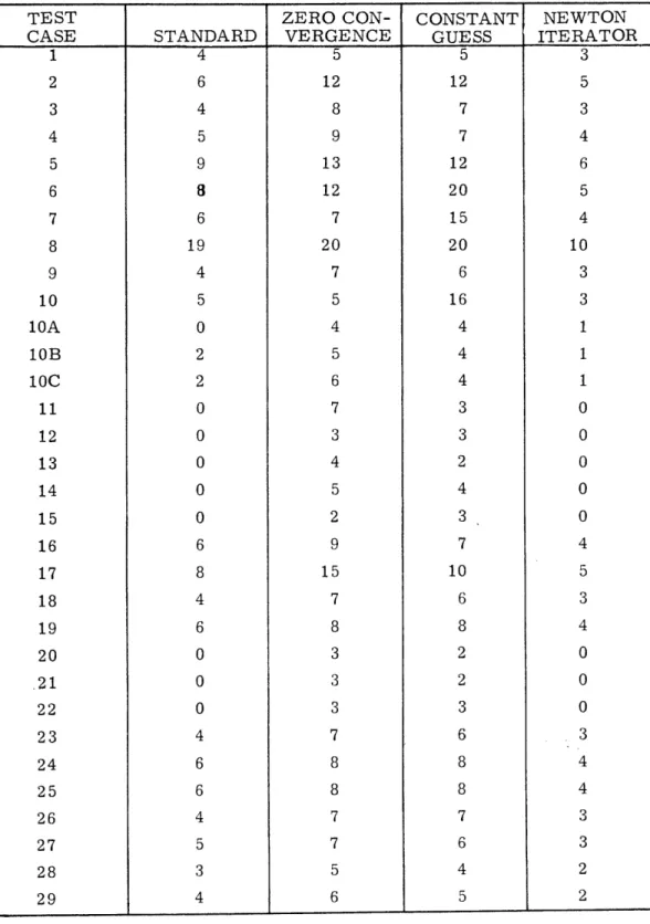
r= TABLE 2.2 NUMBER OF ITERATIONS I TXED I STANDARD 3 0 2 4 4 4 4 4 2 4 12 10 9 4 8 7 2 14 7 5 3 8 12 10 9 8 8 7 4 3 11 3 BOUNDS 3 0 2 4 4 4 4 4 2 4 13 10 9 4 8 7 2 17 7 5 3 8 13 10 9 8 8 7 4 3 11 3 NEWTON ITERATOR 2 0 1 2 3 4 3 3 2 3 6 7 7 3 6 5 2 7 5 5 2 4 6 7 7 5 5 4 3 2 8 2 ZERO CON-VERGENCE 4 2 3 5 6 6 7 5 3 5 14 11 11 8 10 12 3 16 11 12 5 12 17 17 12 10 9 9 7 5 13 6 CONSTANT GUESS 4 3 4 5 5 5 4 5 4 5 18 12 11 6 10 10 5 20 8 7 5 16 18 12 11 9 9 16 5 5 10 5 TEST CASE 1 2 3 4 5 6 7 8 9 10 10A 10B 10C 11 12 13 14 15 16 17 18 19 20 21 22 23 24 25 26 27 28 29 1 ..

-.-TABLE 2.3

COMPUTATION TIME (' SEC )

60 STANDARD 1 <-1 1 2 2 3 2 3 1 2 3 3 3 1 2 2 1 3 3 3 2 4 3 7 2 3 3 3 2 1 3 1 FIXED BOUNDS 1 •1 1 3 2 3 3 3 1 2 3 3 3 1 2 2 1 4 3 4 1 4 3 2 2 4 4 4 1 1 4 1 NEWTON ITERATOR 1 1 1 2 2 2 2 3 21 2 2 2 1 2 1 1 2 2 3 1 2 2 2 1 2 2 3 1 <1 3 1 ZERO CON-VERGENCE 2 1 1 5 6 5 6 5 2 6 7 3 3 2 2 3 1 4 4 7 1 6 4 4 3 4 4 5 2 1 4 1 CONSTANT GUESS 1 1 1 2 3 3 2 3 2 3 5 3 3 2 2 3 2 4 4 4 2 8 5 2 3 4 5 8 2 1 4 1 32 TEST CASE 1 2 3 4 5 6 7 8 9 10 10A 10B 10C 11 12 13 14 15 16 17 18 19 20 21 22 23 24 25 26 27 28 29 . A_ A. . it j Ii i i I i i i

..

TABLE 2.4

LOG10 I ERROR IN FINAL ITERATED TIME I

STANDARD - i2 -15 -15 -13 -9 -8 -8 -8 -9 -9 -10 -9 -5 --9 -7 -5 -8 -8 -9 -9 -13 -11 -10 -9 -5 -7 -11 -6 -8 - 12 -7 -8 FIXED BOUNDS - 12 -15 - 15 - 13 -9 -8 -8 -8 -9 -9 -10 -9 -5 -9 -7 -5 -8 -7 -9 -9 -13 -11 - 10 -9 -5 -9 -11 -6 -8 - 12 -7 -8 NEWTON ITERATOR -11 - 15 - 12 -7 -11 - 13 -8 -9 - 14 - 10 -9 -11 -11 - 12 -11 - 10 x x - 13 -8 - 15 -7 -9 -11 -11 - 13 - 10 -8 - 12 - 13 -11 - 10 ZERO CON-VERGENCE x x x - 13 -13 x -13 x x x -11 x x - 12 x -11 x -11 -11 -9 -15 - 13 -11 -11. -11 - 12 -11 - 12 -14 -14 -11 -13 TEST CASE 1 2 3 4 5 6 7 8 9 10 10A 10B 10C 11 12 13 14 15 16 17 18 19 20 21 22 23 24 25 26 27-28 29 - . .. _ .

TABLE 2.5

LOG10 I RELATIVE ERROR IN FINAL POSITION MAGNITUDE I

STANDA RD - 12 x -14 - 12 - 12 -10 -11 -11 -12 -11 -10 -10 -8 - 13 -10 -10 -12 -11 -12 -11 -13 -11 -10 -10 -8 -11 -11 -11 - 12 - 13 - 12 - 12 FIXED BOUNDS - 12 x - 14. - 12 - 12 - 10 -11 -11 - 12 -11 - 10 - 10 -8 - 13 - 10 - 10 - 12 -11 - 12 -11 - 13 -11 - 10 - 10 -8 -11 -11 -11 - 12 - 13 - 12 - 12 NEWTON ITERATOR - 12 x - 14 - 10 - 12 -11 - 11 -11 - 13 -11 - 10 - 10 - 10 - 14 -11 -11 - 13 -11 - 12 -11 - 13 -11 - 10 - 10 - 10 - 11 -11 -11 - 12 - 13 - 12 - i2 ZERO CON-VERGENCE - 12 x -14 -12 -12 -11 -11 -11 - 13 -11 -10 -10 -10 - 14 -11 -11 -13 -11 - 12 -11 -13 -11 -10 -10 -10 -11 -11 -11 -12 - 13 - 12 - 12 =zero error TEST CASE 1 2 3 4 5 6 7 8 9 10 10A 10B 10C 11 12 13 14 15 16 17 18 19 20 21 22 23 24 25 26 27 28 29 x I I 34 . . .

TABLE 2.6

LOG1 0 I RELATIVE ERROR IN FINAL VELOCITY MAGNITUDE I

STANDARD -12 - 17 - 14 - 12 - 12 -10 -11 -11 - 12 - 11 - 10 -11 -8 - 14 - 10 -10 -11 - 10 -11 - 11 - 13 -11 - 10 -11 -8 - 10 - 11 -11 -11 - 12 -11 - 12 FIXED BOUNDS - 12 - 18 - 14 - 12 - 12 - 10 -11 - 11 - 12 - 11 - 10 -11 -8 - 14 - 10 - 10 -11 - 10 - 11 -11 - 13 -11 - 10 -11 -8 - 10 -11 - 12 -11 - 12 -11 - 12 NEWTON ITERATOR - 12 - 18 - 14 -10 - 12 -11 - 10 - 11 - 13 -11 - 10 - 11 -11 - 14 -11 - 11 - 13 - 10 -8 - 11 -13 - 11 -10 -11 -7 -11 -11 - 11 -11 - 12 -11 - 12 ZERO CON-VERGENCE - 12 - 17 - 14 - 12 - 12 - 11 -11 -11 - 13 -11 - 10 -11 - 11 - 14 - 11 -11 - 13 - 10 -11 - 11 - 13 - 11 - 10 - 11 -11 -11 - 11 -11 - 11 - 12 -11 - 12 TEST CASE 1 2 3 4 5 6 7 8 9 10 10A 10B 10C 11 12 13 14 15 16 17 18 19 20 21 22 23 24 25 26 27 28 29 . , . .

TABLE 2.7 SOLUTIONS TEST CASE 1 2 3 4 5 6 7 8 9 10 10A 10B 10C 11 12 13 14 15 16 17 18 19 20 21 22 23 24 25 26 27 28 29 x (x 103) (meters) 1/2 3. 456 0. 0004 0.221 5. 768 8. 825 1.168 14. 741 16. 905 0.705 7.321 30. 087 30. 099 31. 034 2. 355 11. 222 22. 444 0. 337 11. 222 2. 629 10. 205 0. 271 3.911 30. 081 30. 081 31. 024 12. 411 4. 646 3. 991 1. 6 19 0. 427 6. 676 0. 496 36

-Before one could state that there was a significant improvement a change in the order of magnitude of the error would have to occur. This did not happen. Also, the number of iterations is almost always the same. See Table 2.2. It was also found that this same behavior occurred in all the other Kepler and Lambert methods (i. e in Chapters 3, 4, and 5) when this alteration was made. Hence this variation on the iterator will not be discussed further in suceeding

chapters.

A look at the results in Tables 2.2 and 2. 4 show that for the

"zero-convergence" routine, the accuracy in the final iterated time

did improve but that it usually took a few more iterations. The fact that the number of iterations to achieve zero error did not drastically

increase can be attributed to the fact that zero error is not really

"zero" when using a computer with a finite word length as was ex-plained earlier in Section 2. 4. Due to the increase in the number of

iterations, the computation time of course increases also. See

Table 23. t An interesting result is that the increased accuracy of

the solution (evidenced by the smaller time error) does not decrease the errors in the final position and velocity magnitudes. This is illustrated in Tables 2. 5 and 2. 6 . In fact this parameter of compari-son did not change as a result of any of the variations on the standard

routine for this method. This same behavior reocurred in the other

Kepler and Lambert methods and it was also found that there was no change between the various methods for the same type of routine. We can conclude only that either the errors in the final position and velocity magnitudes are extremely insensitive or that the scheme we

employed to obtain these errors (the numerical integration) is not a good one. In any case, as a parameter for comparison the values obtained in this study are relatively meaningless because they show no change. Henceforth these parameters will not be used for

com-parisons.

t_{The smallest time interval the computer can measure is 1/60 of a}

second (. 0166... ). All computation times in this study are of the

order of the smallest time interval. Therefore a computation time listed in any table is not precise.Nevertheless the results are

con-The results clearly show that the effort of computing an initial guess is worthwhile because it decreases the number of iterations. See Table 2. 2. This method is moderately sensitive to the initial

guess.

The results for the Newton iterator are interesting. Comparing

the number of iterations in Table 2. 2 we can see that the Newton iterator always decreases the number of iterations and the more iterations the standard routine took, the greater was the improvement with the Newton iterator. This suggests good convergence even for very difficult cases or poor initial guesses. One would think that be-cause of the extra calculation of the first derivative the Newton iterator would increase computationtime. However, the results show a distinct trend toward lowered computation time. See Table 2. 3. In addition to this, the Newton iterator improves the accuracy of the final iterated time in many cases (Table 2. 4). The above results strongly advocate

use of a Newton iterator instead of the standard linear inverse inter-polator.t

tIncidently, all Newton iterators in this study employ resetting of bounds on the independent variable.

38

CHAPTER 3

KEPLER z-ITERATION

3. 1 Statement Of The Problem

Stumpff's formulation, Stumpff (1962), of Kepler's problem ist 1 = U₁"z;X) + 7U2 (z;X) + U3(z;X)

r = Fr

+ Gv

t For derivation of these equations see Appendix B or Stumpff(1962).

k I where (3. 1) (3. 2) (3. 3) (3. 4) (3.5) (3. 6) (3. 7)

and t2

3

-o

The new variables z and X are related to x and rx by

rO z = x

t

The solution to Kepler's problem using Stumpff's formulation is quite different from that using Battin's formulation. Instead of finding an x such that a function of x takes on a prescribed value (the time of flight), here we are looking for a z such that a function of z is equal to 1. That is, in the previous chapter the equation of interest was of the form

t = f(x) and in this formulation the equation is

1 = f(z, 't)

t is not an explicit function of z. There is no single t vs. z curve for a given set of initial conditions; on the contrary, for each new specified time, a different curve must be plotted to obtain the solution since the time is included in the definition of the new variables

(Eqs. 3. 11 and 3. 12) and in the parameters 77 and (Eqs. 3. 8 and 3. 9). In the mathematical sense, since both Battin's and Stumpff's formula-tion involve inverting a funcformula-tion, they are identical. One might ask what the advantages and disadvantages of Stumpff's formulation are. One advantage is that the new variables z and are dimensionless. Another is 'that the range of the variable is reduced. In Battin's

formulation the time of flight can range anywhere from 0 sec. to 105 sec. and the solution x may be anywhere between 0 and 10 meters In Stumpff's formulation, however, there is no t and the function of z is always close to 1. As it turns out, z never gets larger than about 4. A third advantage is the fact that in Eq. 3. 1 there are only two parameters and 7, while in Eq. 2. 1 there are three parameters, r0,i,/' and e. One disadvantage is that the physics of the

problem have een lost. Equation 3. 1, although called Kepler's

equation, would never yield a time of flight for a given z directly. The dependent variable time has been submerged in the non-dimensionability of the variables. Another disadvantage is the fact that for each new ·time of flight, one must iterate on a new curve.

Once the initial conditions and the time of flight are given, t

and are determined. In order to investigate the behavior of the right hand side of Eq. 3. 1 we define

f U(Z;X) + 7U2(z;X) + 3(z;X) (U (3. 13)

and plot f vs. z for a typical ellipse, hyperbola, and parabola and observe where f passes through 1. This has been done and the results are given on Figs. 3. 1, 3. 2, and 3. 3. From Stumpff (1962) we have

df H df

ir . Hence, since -d- is always positive f is a monotonically increasing function of z and there is only one unique solution z for each

0 0.4 0.8 1.2 z Figure 3.1 42 1.6 2.0 A 1.6 1.4 1.2 1.0 f 0.8 0.6 0.4 0. 2 A

1.6 1.4 1.2 1.0 0.8 0. 6 0.4 0. 2 0 0.4 0.8 1.; z Figure 3.2 43 2 1.6 2.0

I0 0.4 0.8 1.2 1.6 2.0 Figure 3.3 44 1.6 1.4 1.2 1.0 f 0.8 0.6 0.4 0.2 n

set of initial conditions, such that f = 1.

Since f is a monotonically increasing function of z, we may also use the linear inverse interpolator in solving Eq. 3.1. Once the solution has been found, we calculate F and G from Eqs. 3.4 and

3. 5 and r from Eq. 3. 2. This enables us to calculate A from Eq. 3. 10 and Ft and Gt from Eqs. 3.6 and 3. 7. Finally we find v from Eq. 3. 3.

The maximum and minimum bounds for z can be conveniently

found from the corresponding values for x from Battin's formulation.

For an ellipse, since

2v x max and

i.~~~~~

t

For a hyperbola we max For a hyperbola, we have

I~~~~~~~~~~~~~~~~~~~~~~~~~~~~~~~~~~~~~~~~~~x , ~~i max Px and hence zmax = 5 i max -\ ~ t Y 3. 3 Initial Guess

The initial guess for z can also be found from the initial guess derived for x. The initial guess for x (Eq. 2. 15) was

Ii I

2

r0 2ro 3 r 2r0

Multiplying this by we obtain the initial guess for z

2

r &

v

1-r t

-v OO ₍ vO t 2 _{< O t2 (3. 14)}

2r0 2r0 6r0

A trivial but nevertheless interesting case occurs for t = 0. Eq. 3.1 reduces to z = 1; the guess reduces to z = 1; and the plot of f vs. z from Eq. 3.13 becomes simply the straight line f = z. If we once

again look at the above mentioned nlots of f vs. z given in Figs. 3. 1o .. - - .--..-... I .... --- - -... D_-- - -- ]

3. 2, and 3. 3, we see that for the elliptic case (Fig. 3. 1), the three curves all lie close to the limiting case of f = z. The three times of flight illustrated in Fig. 3. 1 correspond to 1/3, 1/2, and 5/6 of a

period, and hence almost the full range of possible curves for this test case is represented. For the parabola and hyperbola (Figs. 3. 2

and 3. 3), we see that the two curves for the smallest time of flight (on each figure) lie very close to the limiting f = z line and as the

time increases, the curves deviate farther and farther from that line. 3. 4 Convergence Criteria

The same types of convergence criteria are used for Stumpff's

formulation as were used for Battin's formulation. The primary

convergence criteria which will be the same for all formulations is a

-10

-test on f. If (l-f) falls below the standard 10 _{_ -- _ ,-_ .-- --_ _ ---.. _ --- _. -_ _ - I --- ...}the iteration_{_ _ ..._} procedure is haltedt. The test on the 6z produced by the iterator

tThis is consistent with requiring the relative error in time to

converge to 10 .

46

L

-9

employs the 10 criterion (used for x in Battin's formulation)

r0

multiplied by . The test on 6f (corresponding to a test on 6t) employs 10 . Also a maximum of 20 iterations is allowed.

We calculate the U (z;X) for this formulation by first finding C(y) and S(y) as given by Eqs. 2. 30 and 2. 31 with y = yz instead of

2 cx . Then, U2(z;x) = z2 C(y) (3.15) 3 U3(z;X)= z S(y) (3. 16) Also U =

1-

In this way, the same subroutine was used for calculating C(y) and S(y) in both Battin's and Stumpff's formulations.

3. 5 Results

The same types of alterations were made in the basic z - iteration routine as were made in the basic x - iteration routine. See Section 2. 6.

The various routines are listed below.

NEWTON ITERATOR ... Newton iterator

ZERO - CONVERGENCE... zero-convergence criteria CONSTANT GUESS ... constant guess (z = 1)

As shown above, in the constant guess routine, the guess made was z = 1. The increment in the independent variable in the Newton iterator is made as follows:

1 - f (Zold) Znew = Zold +

old

where

df old = UO( old) d) d ) +U(olU2(zold)

U 0= 1 - U2

U1 = z U 3

The results are given in Tables 3. 1 through 3. 4. The results of the zero-convergence routine show the expected increase in the accuracy of the final iterated time (Table 3. 4) and the accompanying increase in the number of iterations (Table 3. 2). It is interesting to note that the final error in the iterated time went to "zero" almost

every time.

Comparing the standard routine to the routine which used a constant guess of z = 1 we see that the number of iterations usually increased by only one or not at all. The reason is that many solutions are close to z = 1 (Table 3. 1). This formulation seems to perform well for a constant initial guess but there must be a high sensitivity of f to z in Eq. 3. 13 since even when the solution is almost exactly equal to the guess (which occurs very often) a finite number of

iterations is always performed.

The results from the Newton-iterator routine are very

encour-aging. The number of iterations is consistently reduced and the improvement is greater for cases where the original number of

iterations was large. Tne accuracy n tne Imal time also increased

in a majority of cases and the computation times showed a definite tendency to decrease from the standard routine to the Newton iterator.

From the above discussion it appears that the zero-convergence

criteria routine is very effective in decreasing the error in the final iterated time at a slight cost in computation time, and the Newton iterator has the most improved performance over the standard routine of all the alterations made.

48

L Aj

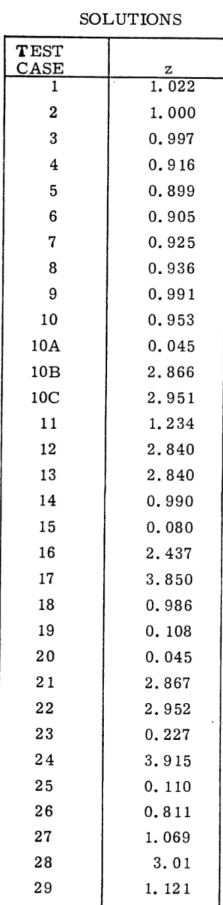
TABLE 3. 1 SOLUTIONS TEST CASE 1 2 3 4 5 6 7 8 9 10 10A 10B 10C 11 12 13 14 15 16 17 18 19 20 21 22 23 24 25 26 27 28 29 z 1. 022 1. 000 0. 997 0. 916 0. 899 0. 905 0. 925 0. 936 0.991 0. 953 0. 045 2. 866 2.951 1. 234 2. 840 2. 840 0. 990 0. 080 2. 437 3.850 0. 986 0. 108 0. 045 2. 867 2. 952 0. 227 3. 915 0. 110 0. 811 1. 069 3.01 1. 121 t i iI I I Ii i

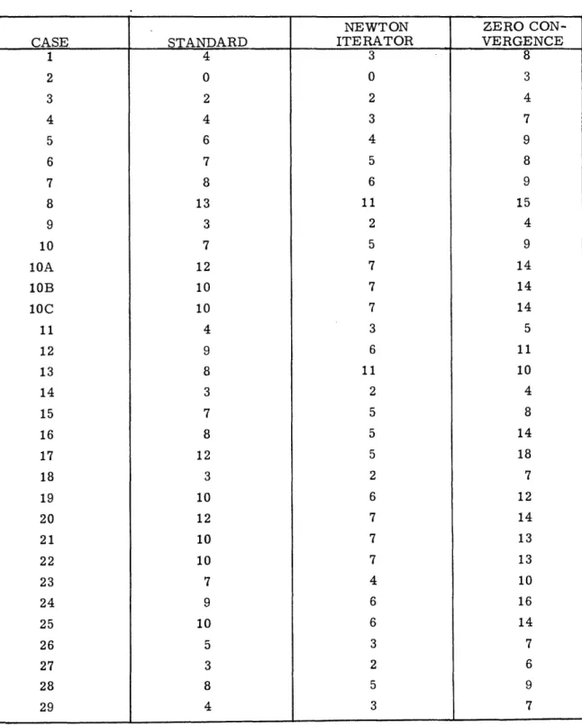
TABLE 3.2 ITERATIONS STANDARD 3 0 2 4 4 4 4 4 2 4 12 10 9 4 8 7 2 14 7 5 3 8 12 10 9 8 8 7 4 3 11 3 NEWTON ITERATOR 2 0 1 2 3 4 3 3 2 3 6 7 7 3 6 5 2 7 5 5 2 4 6 7 7 5 5 4 3 2 8 2 ZERO CON-VERGENC E 4 2 4 4 5 6 5 5 3 6 13 11 11 5 9 9 5 16 9 9 4 9 13 11 11 9 11 9 6 5 13 5 CONSTANT GUESS 3 1 2 4 3 4 4 5 3 4 12 11 10 5 9 12 3 14 8 7 3 8 12 11 10 8 9 7 5 4 10 4 50 TEST CASE 1 2 3 4 5 6 7 8 9 10 10A 10B 10C 11 12 13 14 15 16 17 18 19 20 21 22 23 24 25 26 27 28 29 _ .

TABLE 3. 3

COMPUTATION TIMES (1/60 SEC) STANDARD 1 <1 1 2 2 2 3 3 <1 3 3 2 2 1 2 2 1 3 3 4 1 4 2 2 2 5 3 3 1 1 4 1 NEWTON ITERATOR 4 <1 1 2 2 2 2 1 3 2 2 1 1 1 1 2 2 3 1 1 2 1 2 2 2 3 2-1 <1 3 1 ZERO CON-VERGENCE 3 <1 3 2 4 6 4 4 2 4 6 3 3 1 2 2 1 4 4 5 1 4 3 2 2 4 5 4 2 4 4 2 CONSTANT GUESS 1 1 1 2 2 2 3 3 1 3 3 3 3 2 2 3 <i 4 3 4 1 4 3 3 2 3 5 3 2 1 4 1 TEST CASE 1 2 3 4 5 6 7 8 9 10 10A 10B 10C lOC 11 12 13 14 15 16 17 18 19 20 21 22 23 24 25 26 27 28 29 -.

TABLE 3.4

IERROR IN FINAL ITERATED TIMEI

CASE 1 2 3 4 5 6 7 8 9 10 10A 10B 10C 11 12 13 14 15 16 17 18 19 20 21 22 23 24 25 26 27 28 29 STANDARD -11 - 15 - 15 x -9 -7 -8 -8 -9 -8 - 10 -9 -5 -9 -7 -5 -8 -7 -9 - 10 - 13 -11 - 10 -9 -5 -7 -11 -6 -8 -11 -7 -8 NEWTON ITE RATOR - 10 - 15 - 12 -7 - 10 - 12 -7 -8 x -9 -8 - 11 - 11 - 11 - 11 - 11 x - 11 - 11 -8 x -7 -8 x - 10 x -9 -8 - 12 - 13 -11 -9 ZERO CON-VERGENCE x x x x x x x x x x x x x x x x x -11 x - 10 x x x x - X10 - 10 - 12 - 13 x - 11 - 13 - 13 x = "zero" error 52 LOG1 0 I ___ S .

CHAPTER 4

KEPLER U1( )-ITERATION

4.1 Introduction

The most direct and obvious method of obtaining x, given t, from Kepler's equation is to guess the x and evaluate the three universal functions U1, U2, and U3 as done previously. Therefore

some method of evaluating infinite series expansions to a desired accuracy must be implemented. (This is fully discussed in our

_:I.-;_ % A A A

IL1

xU-daLLU11 1ncLUU. ny iniiniiLe seVries evaluacdLLU LKeb riLMe anu

may cause computational difficulties. For 'the x-iteration, the difficulty is compounded since at least 2 series must be evaluated.

Battin (1968-69) has shown how a method of solution of Kepler's equation may be derived which avoids the evaluation of any infinite series. That is, the equation is worked into a form in which the single

irl.lo c nf rL ,v ·nri-lJ.l'. ^n h J'nIA +r1L 1wlP h ^ rlfP f 1The 1 rni%.ran1 TT

g x

functions, in particular U

(4).

x x

expressed in terms of U1(,), except a particular combination of U3 )

and U1(4). This combination is then expressed as the solution of a

well known hypergeometric differential equation. This solution, a hvnerbnnomtri flnrftinn i thpn PxnrAP.sPd in vrv rnnvenient rnidlv

,,

-j

5

YI

convergent, continued fraction expansion in terms of U1(4). Therefore,

the time of flight equation can be evaluated for a given value of the single variable U1(4). We have traded the problems of calculating at least

two infinite series for any difficulties associated with this continued

T II

an initial point for the iteration. As we will show, the evaluation of the continued fraction can present no problem, while in some cases, the initial guess can be difficult to make with sufficient accuracy.

4. 2 The Method Of Solution

The equation used is (from Appendix C, Eq. (C. 2))

r

.wU

X

U(X)

32()

U

(

qZ

0 A

iT1

F

(1,

The variable U ( ) can_{1 4} be expressed as

2 UI( ) = 1 -- 6' 2 2

(a x

+ 57

. ^

-V,( L

The first necessity we must face when we want to begin the

iterative procedure is that of determining an initial guess. It turns

out that for this method of solution of Kepler's problem the guess is critical to the success of the iterative procedure, but is unfortunately difficult to compute in certain circumstances. Since the discussion of the guess for this method is very lengthy because of its importance, it will be presented in a later section.

4. 3 Convergence Criteria And Bounds

The next step in the implementation is to define what convergence

criteria we will use to terminate the iteration.

The primary convergence factor demanded that the iterated

time agree with the desired time to within 1010 of the desired time.

-16

This factor is reduced to 10 in another test run to compare the resulting iterations as well as the accuracy in the final position and velocity.

16

A convergence factor of 1016 was used on the difference between the last two calculated times so the denominator of the iterator did not go to zero. This was a standard criteria for all test runs made.

The criteria used to determine when the change in the independent variable was too small to change the time was in part a result of the knowledge of the criteria used for the generalized anomaly, x, (see Chapter 2). The numbers used were obtained by finding the

differential of U1(4) in terms of the corresponding differential in 6x.

There results

[U1()] = U0() 6x (4. 1)

We therefore must define the limits on the variable U0(4) from the definition of Un(). (See Appendix A. ) It is obvious that for ellipses the maximum value of U0(4) is 1. 0. Furthermore, under the

is 50, (see Ref. 12) we can determine the maximum value of U0(4) for hyperbolic paths as follows:

XU

UO()MAX cosh (H -4 JAH~H% = cosh( '4 50 )

MAX,,

U (X

U0 "I)MAX = 3.01

In our case a value of 5.0 was chosen to insure no difficulty. Returning now to Eq, (4. 1) we have

6 [u 1(X)] 6 U1 4) ] 1 6x = 6x 4 > 0 a < 0

The values used for 6_{x wer}

-9

and 10 for moon centered pa'ths.

e 10 8 for earth centered trajectories

Finally to determine the maximum and minimum values of U1 (x), we examine the definition of U1() in terms of trigonmetric

and hyperbolic sines.

Examining first the elliptic case rewritten in the form sin( E4

4 J

where E is the standard eccentric anomaly for ellipses, it is obvious that 1 > U(T) > 0 a > 56 T I. ()

and these are precisely the bounds used in the elliptic case.

For hyperbolic trajectories we have

U1(X) =

H-Ho

sinh( )

4VT

< O

Using the maximum value of H - Ho employed above, we can show₀

1 MAX

-2.87

However, the maximum we used difficulty. Therefore we have,

0 > U

substituted 3. 0 for 2. 87 to insure no

!(E) > < 0

Typical numbers for the maxima can be found using the semi-major axes of the test cases listed in Chapter 2. The units for U1(4) are,

1/2 of course, (length)

Finally, after the iterative procedure has resulted in the correct

value of U (4), we can use the identities in Appendix C to determine all necessary universal functions involved in the vector position and velocity equations:

r = [1 U

(x) + t

-

U

(x)

-=0 + [ 1 -

+ [1- U

r

(x)

All quantities in Eqs. (4. 2) and (4. 3) will then be known and r and v can be determined. The solution will then be complete.

4. 4 Evaluation Of The Hypergeometric Function

We have shown that we can express the universal form of the time of flight equation in terms of the value of Ul(4), (see Appendix C). To accomplish this, we have to evaluate the function

Q

U-U3()

in terms of a hypergeometric function; that is

8 1 51 U0 -1

Q

8

h

F

[1,

-;a;

x

i

Since it has been found that the ontinued fraction renresentatinn of this F converges slowly, (Battin 1968),we are interested in transforming this solution into one with more rapid convergence properties.

Improved convergence will be necessary if this method of solving Kepler's equation is to be competitive with series expansion methods.

For this purpose, we note first that hypergeometric functions

can be evaluated by infinite series or by continued fraction expansion. If we examine the series representation we can show that the series does indeed converge and then see how to improve this convergence.

In general we have,

F(a, 8;y; q) = 1 +

+,f

(+

q

. 1"2.12+- 1)

a(WU+ l) 1) (&+ (P I)+ )to+ )

1+ 23'7y(y+ 1)(y+ 2) +(4 4) 4. 4)

we know 'that such a series converges absolutely for IqI <1. Therefore if we prove that q falls in this region for all possible cases, we can

feel secure in using this method of solution.

For this purpose, we observe first, 'that in our case

U0() - 1

q

Then using the limits on U0( ) discussed above we can easily show 'that

0 > q >- 1 for 1 > U ( 4) > 0

and

.503 > q > 0 for 3.01 > U0(4) >1

Returning now to Eq. (4. 4) we can see that this infinite series representation does indeed converge for all possible values of U (). We can further see that by increasing v in the denom-inator of the terms of 'the infinite series, the rate of convergence can be improved. We would also expect this same factor, , to

improve the convergence of the continued fraction representation. (The relation between the series and continued fraction reDresen-tations will not be discussed heret.)

For this purpose, we begin with the following identityt (y- o- B) F(c, 8; ¥; q) + (1 - q) F(t + 1, ; ,; q)

- (v- R) F(oy, 8- 1; Y; q) = 0 (4. 5)

T For a complete discussion see Battin(1968)

t The identities used here are taken from Battin (1968-69). Reference 'to sources of these identities are made in Battin (1968).

j i i I i i i

1

with = - _{Y .} B= 1, 1 = 2

2 and, (as before)

0(4)-

1

where we have defined

= U0()

Now, to increase a, we use another identity

y(1- q)F( , 8; ; q) - yF(a- 1, 8; y; q)+(y- )q F(lal , y+1, q) = 0 (4.6)

with c=l, 8= 1 5

to obtain

F(1,

½;

7

; q)

_(w

-7 -72 - w 1) F(2, 1; 7; q)

By recursively applying this same identity, Eq. (4. 6),we would have

1 w- 1

F(1, ; ; w + ) w+l₂

We could increase y to any desired size. The results of several

successive applications of this formula are discussed below.

Battin(1968) has shown how to evaluate a hypergeometric function of the form

F(, 1; + N;

w-

60 r = 3 + I 2 ) ( 4 T -w- T T TZ i i 1I i I (1- 1 ) w - F 11 +

The final result, which is used here is given by: 1 7 w - 1 2N+5

F(

_{, 1; + N;}

) = 9N

- -

(4.7)

n-

+

-

(4.8)

and w = U() as before.

To evaluate the series of Bn's we proceed as follows. We select i

,tlr ' ',

I

h

t"-A

+."

';

a

cS"A"

1

=

t

n

TPh"i

'T';.i.'fi1'

vl']

Ic.

to terminating the continued fraction at n levels and dividing out the succeeding levels, i. e. working backwards. ) We then calculate Bn - 1' This becomes the new Bn and a Bn 1 is calculated from

this. The process continues until B2 is calculated at which point

the hypergeometric function is evaluated.

It was pointed out before that increasing (or N in Eq. (4. 7)) improves the rate of convergence of the continued fraction expansion.

1 f7 + N w 1

TVF we senerate a senuence of algorithms for F(-k. 1: ;,

...

...

-

-,

w

+ 1'

_ 8 1 , 1 5_

i )

4+

5 [U 4)]

q=

For N = 0, we can use the identities presented above to show 1 5 w - 1 1 w- 1 1 7 w- 1 F(1,-

_~'

_7'2'

_ww

_'+

2 ' 'E' w+1

From Eq. (4. 8) we can further show

5B 5 w+ 1 - B N = 0

5 -

B

w- 1

For N = 1 we can show

w +=

1 [1

(1 - B

]

i'Pinnllv fr N = 2

=

F

Q w+l 10 '

(where, of course, Eq. (4. 8) is employed using the corresponding value of N. )

As N increases we should have to make fewer evaluations of the recursive relation for 'the Bn's to get the same accuracy. That is if we specify that we want this representation to give a result correct to a certain digit after the decimal point, we must determine how many levels are required to leave this digit unchanged in successive evaluations of B1. Further levels can only change

62