Common cause analysis : a review and extension of existing methods

(1)

COMMON CAUSE ANALYSIS:

A REVIEW AND EXTENSION OF EXISTING METHODS by

C. He ising, N. Rasmussen and C. Mak

Energy Laboratory Report No. MIT-El 82-038 October 1982

(2)

COMMON CAUSE ANALYSIS:

A REVIEW AND EXTENSION OF EXISTING METHODS

by Carolyn D. Heising Principal Investigator Norman C. Rasmussen Co-Investigator Cho H. Mak Research Assistant Energy Laboratory and

Department of Nuclear Engineering Massachusetts Institute of Technology

Cambridge, Massachusetts 02139

...

A. Code Description ... B. _{Sample Problems ...}

B.1 Warehouse Fire Protection

System (FPS) ... B.2 Millstone I Automatic Pressure

Relief System (APR)... C. _{Propagation of Uncertainty in MOBB ...} IV. Cutset Susceptibility Concept for Common

Cause Analysis ... A. B. C. D. Method Description... Code Description...

Sample Problem: Warehouse FPS... Comparison of DPD Uncertainty Treatment

With Method-of Moments ... V. Summary/Conclusions... References... 5 5 11 15 20 20 23 23 35 35 43 43 52 54 72 72 79

(7)

List of Figures

Figure

1: State Transition Diagram for Repairable

2-Component System ... 2: State Transition Diagram for Non-Repairable

2-Component System ... 3: Flow Diagram of MOBB Code... 4: Schematic Flow Diagram of the FPS... 5: System Fault Tree ... 6: Floor Map and Susceptibility Maps... 7: Fault Tree for APR System for Human Error... 8: APR System Analysis ... 9: Behaviour of Various Lognormal Function

Options... 10: Plot of Resulting Curves of Top Event

Unavailablity... 11: Environmental Stress Curve ... 12: Cutset (Component) Environmental

Susceptibility Curves... 13: Result of Environmental Stress Analysis

on System rutsets ... 14: Modified Warehouse FPS With Added Diesel

Generator ... 15: System Fault Tree ...

16-22. Cutset Fragility Curves... 23. Seismicity Curves... 24: System Failure Probability Distribution

Due to Seismic Events... 25: Method-of-Moments Used to Combine

Cutset Fragility Curves...

Page .... 16 .... 16 .... 21 .... 24 .... 25-26 ....27 .... 36 .... ...37 ... 41 ... 44 ... 53 ... 53 .. ... 53 ... 56 ... 5...7-59 ... 61-67 ... 68 ... 69-71 ... 76

(8)

I-V: VI: VII: VIII: IX: X: XI: XII: XIII: XIV: XV: XVI. XVII: XVIII XIX: XX: XXI: XXII-XXIV: XXV: List of Tables Table _Page

Review of Project Tasks... 2-4 Dependent Failure Classifications...7-8

Methods for Modelling Dependent Failures...9

Generic Causes of Environmental Stress...22

Failure Mode Codes...28

Susceptibility Domain...28

Component Code... 30

Common Cause Failure Data ... 31

Qualitative Failure Characteristics... 32

Output from MOBB... ... ... 33

Basic Events... MOBB with Monte Carlo ... MOBB with Method-of-Moments... Mathematical Formula for Various Lognormal Functions Employed in Method-of--Moments... Sample Unavailability Expression: Results of Comparison... Cutset Fragility Concept Applied to Analyze CCF... .34 .38 .39 ... 40 ... 42 ... 55 Cutset Definition for FPS with Top Event Boolean Expression (System S3). Results of DPD Code on FPS Problem ... Comparison of Approaches for Combining Cutset Fragility (Susceptibility) Curves ... ... ... 60

S..73-75 ...77

(9)

I. Introduction

As stated in the proposal, the purpose of this research

project was to further assess and extend the MOCUS-BACFIRE computer code, first combined by Modarresin 1979(1) to provide the utilities with an effective and powerful tool for analysis and evaluation of common cause failures(CCF) in a system represented by its fault tree diagram.

The project has accomplished the following tasks:

(1) Assessment and comparison of MOCUS-BACFIRE, BACFIRE-II and COMCAN-II codes;

(2) redefining existing criteria for identifying CCFs and incorporating them into the selected code;

(3) selection and incorporation of a more sophisticated common cause quantification method; and

(4) evaluating sample problems chosen by the utility sponsors. A detailed review of each of the specific contract tasks is presented in the attached Tables I- V.

The expected benefits of this work to the utilities are to obtain codes which are:

(1) capable of identifying common cause failures directly from the fault tree diagram;

(2) inexpensive and easy to operate;

(3) capable of automatically generating common cause candidates which are significantly contributing to the failure of the

system due to common cause failures;

(4) capable of calculating the top event probability (or

unavailability) by considering both random and common cause failures;

(5) especially suited for man-machine communication and its advantages.

(10)

Task 1:

Status:

Conclusion:

2

TABLE I

REVIEW OF PROJECT TASKS

Assessment of existing qualitative common cause failure analysis codes that use generic cause approach to identify common cause candidates from minimal cutsets

-COMCAN versions -BACFIRE versions -Sets (Sandia)

Completed April, 1981

BACFIRE is preferable over the others, and is the code selected for integration with quantitative evaluation methods. TABLE II Task 2: Status: Conclusion: Product:

Choose an appropriate quantitative method to quantify the common cause candidates and evaluate the system unavailability.

Completed May, 1981

Beta-factor method developed by Karl Fleming at General Atomic for HTGR-PRA is perferable. This method was integrated into the modified BACFIRE

packaqe. _{(It has also been refined and updated).}

MOBB code.

(11)

Task 3: Status: Conclusions: Documentation: Product: Task 4: Status: TABLE III

Implementation of the qualitative method chosen to quantify common cause candidates and evaluate system unavailability.

Completed August, 1981

Sample problems were run using the MOBB code. These included analyses of the following two

systems:

-Auxiliary feedwater system (AFWS) -Fire protection system (FPS)

-Cho Mak's SM thesis

-Paper for Portchester PRA meeting Useful examples to guide utility efforts in

systems analysis.

TABLE IV

Review and further extend the capabilities of the code to include uncertainty analysis, data collection and interpretation, redefine parameters and failure criterion.

Completed.

Additionally, a separate code for uncertainty analysis using the DPD method of seismic risk analysis

(HADES code). Examples have been run. Preliminary

Conclusions: -Monte Carlo Method applicable -Has been incorporated into MOBB. -Sample problems run.

Further work needed (beyond this project scope);

-More efficient method required to reduce computer time.

(12)

TABLE V

Use of final version of the code for a detailed common cause failure analysis.

Completed. Date of Completion: Final Product: Documentation: End of September, 1982.

Revised code on tape for use in IBM-370 system. -Project final report

-Technical paper to be submitted to Reliability Engineering Journal

Task 5:

(13)

5

II. Quantitative Common Cause Failure Analysis A. Dependent Failure Analysis

Dependent failures are an extremely important aspect of risk quantification and must be given adequate treatment to avoid gross underestimation of risk. Risk estimates can be many orders of magnitude off if the possibilities for dependent failures are overlooked. An example of how crucial common cause dependencies

can be was the case of the Titanic; it was thought to be "unsinkable" because it was designed to have so-called "independent" compartments

in the bottom hull of the ship. The Titanic sunk because the depen-dency between compartments was overlooked by the ship designers. This is an important lesson to all reliability engineers.

There are two major types of dependencies between events: 1. Actual physical dependencies between systems and/or

events (e.g., seismic event and containment failure events.) These dependencies are discussed in Section 3.7, "Analysis of Dependent Failures," PRA Procedures Guide, NRC, 1982, K.N. Fleming, author. (1)

2. "State-of-knowledge" dependencies for nominally

identical components whose failure rates are presumed identical. This type of data-related dependency is discussed further in Section 16.5, PLG Handbook, p. 109 on. (2)

The first kind of dependency is what is most often studied in common cause analysis. The second kind is somewhat new in the sense that it has only recently been identified. It is related

(14)

to the subjectivist (or Bayesian) theory of probability.

Mathematically, two failure events A and B are said to be dependent if their frequency, p, satisfies:

q(A and B) = p(A).(BjA) r _p(A)-(B) (1) In other words, the frequency of concurrent failure events A and B (4(A and B)) cannot be expressed simply as a product of the unconditional failure event frequencies (A) and p(B). Dependent failures are defined into different groups as shown in Table VI(1) with methods which have been used to handle each shown in Table VII.

Analysis of Intercomponent Dependencies

The type of common cause failures that are of most interest here are those classified as Type 3 in Table VI, or intercomponent dependencies. Before the quantification of the system unavailability can be completed, it is necessary to analyze the possibilities for dependencies among the basic component failures.

(15)

TABLE VI

DEPENDENT FAILURE CLASSIFICATIONS (1)

Type 1 Common Cause Initiators (external events) These include external and internal events that have the potential for initiating a plant transient and increase the probability of failure in multiple plant systems. These events usually, but not always,

result ihsevere envirornmental stresses on components and structures. Examples include fires, floods and earthquakes.

Type 2 Intersystem Dependencies These are events or failure causes that create interdependencies among the probabilities of failure of multiple systems. States another way, intersystem dependencies cause the conditional probability of failure of a given system along an accident sequence to be dependent on the success or failure of systems that precede' it in the sequence. There are several subtypes of interest in risk analysis.

Type 2A Functional Dependencies These are dependencies among systems that follow from the plant design philosophy, system capabilities and limitations, and design base. One example is a system that is not used or needed unless other systems have failed. Another is a system that is designed to function only in conjunction with the successful operation of other system.

Type 2B Shared Equipment Dependencies These are dependencies of multiple systems on the same components, subsystems, or auxiliary

equipment. Example are: 1) a collection of pumps and valves that provide a coolant injection and a coolant recirculation function when the functions appear as different events in the event tree,

and 2) components in different systems fed from the same electrical bus.

(16)

TABLE VI, cont'd (1)

Type 2C Physical Interactions These are fialure mechanisms, similar to those in common cause initiators, that do not cause an initiating event but nonetheless increase the probability of multiple system failures occurring at the same time. Often they are associated with extremeenvirormental stresses created by the failure of one or more systems after an initiating event. For example, the

failure of a set of sensors in one system can be caused by the excessive temperature resulting from the failure of a second system

intended to cool the heat source.

Type 2D Human Interaction Dependencies These are dependcies introduced by human actions, including errors of omission and commission. The persons involved can be any~'ne associated with a plant life cycle activity, including designers, manufacturers, constructors, inspectors, operators, and maintenance personnel. Such a failure occurs, for example, when an operator turns off a system after failing to correctly diagnose the plant condition.

Type 3 Intercomponent Dependencies These are events or failure causes that result in a dependence among the probabilities of failure of multiple components or subsystems. The multiple failures of interest in risk analysis are usually within the same system or the same minimal cutset that has been identified for a system or an entire accident sequence. Subtypes 3A, 3B, 3C and 3D are

defined to correspond with subtypes 2A, 2B, 2C and 2D, respectively, except that the multiple failures occur at the subsystem and

(17)

9

TABLE VII

METHODS FOR MODELLING DEPENDENT FAILURES (1)

Dependent Failure Type

Type 1: Caommon Cause Initiators

Type 2A: Intersystem Functional Dependencies

Type 2B: Intersystem Shared Equipment Dependencies

Type 2C: Intersystem Physical Interactions

Type 2D: Intersystem Human Interactions

Type 3: Intercomponent Dependencies

Recommended Method of Modelling

1-a Event Specific Models

3-a Qualitative Search Procedures 1-b Event Tree/Boundary Condition

Method

1-b Event Tree/Boundary Condition Method

1-c Fault Tree Linking Method 1-a'tvent Specific Models

3-a Qualitative Search Procedures 1-b Event Tree/Boundary Condition

Method

1-c Fault Tree Linking Method 1-d Fault Tree Cause Analysis 1-e Human Reliability Model

1-d Fault Tree Cause Analysis 2-a Beta Factor Method

2-b Binomial Failure Rate Model

.m~c -mia.r---r~*--- ~4-L YI~YYL1YU -mr~).^~--I~VPIIV I~I"L-l~Olr~)l7 "~LM

-_

(18)

-10

Consider a system of three components A, B, and C; let the reliability block diagram be:

The corresponding system unavailability, Q, is: Q = P(A and B) + P(C) - P(AnB AC)

= P(A)* P(BIA) [l-P(C AB)] + P(C)

where

P(x) = availability of component x

P(ylz and t) = unavailability of component y given components Z and t are failed;

P(BIA)>>P(B) in this example. There are three basic approaches to CCFA:

(1) Develop causes explicitly in fault trees or cause tables (primarily qualitative approach)

(2) Beta-Factor Method (Parametric)

(3) Binomial Failure Rate Model (Parametric)

Tne greatest limitation of approach (1) is that in an effort to

ensure completeness, an intractable number of dependencies are identified. Taken separately, these dependencies can often be discounted on the basis of a perceived low occurrence probability. Experience shows, however, that as a class they cannot be dismissed. Thus it is difficult to know which common cause candidates are

important and which are not. Therefore, we must go to quantitative procedure, as is done in this project, such as the Beta-Factor

method. Before doing this, however, we review some previous work in this area.

(19)

B. Previous Work on Quantification of Common Cause

Unavailability calculations of engineering safety features and risk assessment studies (3,4) revealed the importance of considering potential common cause failures in estimating the probability of failure of redundant systems. It is a well-recognized fact that reliability predictions of redundant systems are overestimated when the potential for common cause failures is not properly accounted for. _{In fact, the RSS amply demonstrated that CCF may} contribute the most to system unavailability.

The state-of-the-art of CCF analysis up to 1979 has been reviewed by Rasmussen et al. (5). Hayden (6) separated CCF's into component and system failures and categorized them in terms of generic

failure mechanisms such as design error, human error and generic events. Apostolakis (7) used a constant hazard rate for reliability and redefined the hazard rate by using a point estimate of the

conditional probability that a unit failure is due to a common cause failure.

Certainly the most thorough CCF analysis was performed as part of the RSS in each of the following analysis steps:

- Event tree construction - Fault tree construction

- Fault tree quantification - Event tree quantification

- Special engineering investigations

Computerized efforts in the qualitative and quantitative procedure of common cause failures were begun with special emphasis after

the publication of the RSS. Burdick et al,(8) reported on the COMCAN

(20)

code. This code is designed to aid in the qualitative determination of:

(1) single secondary events that could fail an entire minimum cutset, given all components in the cutset share the same susceptibility location.

(2) Common links among components such as common circuitry, common maintenance personnel or common manufacturers for all components in a cutset.

As a result, COMCAN requires as one of its inputs a set of minimal cutsets which have been obtained by some other qualitative

analysis code. It is quite apparent that for large fault trees with a high degree of replication and the possibility of several

common cause failures, the computational efforts involved in the minimal cutset sorting become tremendous, if not impossible, due to the large amount of minimal cutsets. Modarres et al. (1) have developed a computer code package to resolve this difficulty by

coupling the cutset generator code MOCUS (9) and common cause failure analysis code BACFIRE (10) to obtain the MOCUS-BACFIRE Package.

The BACFIRE Code is a newer and more adequate version of the COMCAN Code. However, a newly developed version of the COMCAN Code, which is called COMCAN-II (11), has been recently developed to directly evaluate common cause failures from the fault tree diagram.

Similarly, BACFIRE was extended to obtain the BACFIRE-II code (12). Therefore, the codes COMCAN-II, BACFIRE-II and MOCUS-BACFIRE have relatively similar capabilities. However, they employ different algorithms to determine CCFs, and the efficiency and limitations of

(21)

these codes had not been compared and assessed yet.* The development of the COMCAN methodology laid the ground for the first time with basic rules which will be common to all future efforts involving common cause handling. The most important thing which was realized during the course of the development of this code is the recognition of the importance of generic classification. The possible physical sources for a specific secondary event can develop into an

absolutely endless list. Only a unique generic classification makes the search for minimal cutset sharing susceptibilities a tractable task. For this purpose, a preprocessor has been implemented in COMCAN which needs as input generic categorization of secondary causes.

A special category has been added which links conditions among components to locate potential common cause failures of minimal cutsets. The other three categories considered by COMCAN are:

- Mechanical or Thermal - Electrical or Radiation - Chemical or Miscellaneous

Recent studies (13, 14) have shown that the criteria for

identifying a cutset as a common cause candidate in the COMCAN code is not unique and sufficient for a complete CCF analysis. It is

important, however, to select an adequate set of CCF criteria in order to obtain a set of adequate common cause candidates.

The review of computerized qualitative common cause failure analysis suggests the following conclusions. First, the original COMCAN code approach, which uses the complete minimal cutset

information, has no potential for further development because of They have been compared in this project.

(22)

a prohibitive amount of cutsets that must be input to the code

for a large fault tree. Second, the codes MOCUS-BACFIRE and COMCAN-II eliminate the necessity to input the cutsets. Therefore, instead of the cutsets, they require the fault tree to be input. However, they had not been fully tested and assessed.* A careful revision is required to establish a set of new criteria for identification of common cause candidates from the cutsets.

The state-of-the-art in common cause quantification is

largely determined by the work described in WASH-1400 and the new developments by Vesely (15). Whereas in WASH-1400 common cause failure probabilities were evaluated using upper and lower proba-bility bounds, Vesely showed that common cause failure probabilities can also be evaluated directly by using the multivariate exponential model developed by Marshal and Olkin (16). For this purpose, Vesely developed a statistical estimation technique for cases where common cause failures are repairable. Two special cases were examined, the constant failure rate case and the binomial failure rate case. A BWR scram system served as an example. In another paper, Johnson and Vesely (17) applied the same technique to the common cause

analysis of valve leakages. In both papers, actual data were used from EPRI records and Licensee Event Reports (LER), respectively.

It should be noticed that the quantification model used is dependent upon the data population and presupposes that the components from a given defined population are subject to similar failure causes.

Fleming and Raabe (18) compared GA's approach (known as s-method) to both aforementioned methods (i.e., RSS and Vesely's methods).

(23)

15

The objective of their paper was to show the validity of the common cause coupling B-method as compared to the bounding technique

of the RSS and the multivariate exponential distribution of Vesely. Modarres etal. (1)have recently studied a method to quantify

CCF affect by using a Markovian approach. They used exponential distributions to model and evaluate the failure probability of cutsets due to both random cause and common cause failures. A simplified aux-feed system served as an example, and failure probabilities were close to that predicted by the RSS bounding method.

C. The Beta-Factor Method (18) Definition of the Beta Factor

The Beta-Factor of a component event is defined as the fraction of all common cause failures to the total number of failures, which include both independent and common cause failures. Since most components are susceptible to more than one common cause, the level of susceptibility is used to specify the relative occurrences of a

secondary failure of a component.

The common cause candidates identified can be considered as a subsystem. To quantify the common cause candidates, Markov models are applied to these subsystems. The failure and repair rates are assumed to be exponentially distributed. A non-identical repairable two-component system with common cause failure is used as an example. The Markov state transition diagram is shown in

Figure 1. The following assumptions are made to develop the model:

(24)

Figure 1

State Transition Diagram for Repairable 2-Component System

P₀ (t) = probability at time t, both units are

operational

Pl(t) = probability at time t, only unit i has failed,

- for i = 1,2

f P₃(t) = probability at time t, both units have failed

/ 1= independent failure rate of

/ unit i, for i = 1,2

) A c= common cause failure rate

A= repair rate of unit i, for

/J i = 1,2

3

3= repair rate of both units,

1 and 2 Figure 2

State Transition Diagram for Non-Repairable 2-Component System

(25)

(1) Common cause and independent failures are statistically independent,

(2) common cause failures can only occur with more than one unit, and they fail simultaneously.

The system of first order differential equations can be written for the model as:

2 3 P'(t) =-(i=lXi ( t ) +X c ( t ) ) P O (t ) + i = Pi ( t ) i ( t ) (1) p'(t) =-(A2 (t)+ l )P (t)+P (t)13(t) 2 (t)+P1(t (t) (2) P'(t) =-(Al (t)+ 2(t))P2 (t)+P(t)A t)+P (t) 2 (t) (3) 2 2 P'(t) =-(Pi=li (t)+ 3 (t))P (t)+ Pi(t(t)+P (t) (t) (4) 3 i=Pi(t) = 1 (5)

If all the failure and repair rates are time independent and a set of appropriate boundary conditions are given, equations (1) to (5) are then a set of linear differential equations which can

be solved by using Laplace transform techniques. The system unavail-ability at time t is P3 (t) for a 2-component system in parallel.*

Beta-Factor Method

The total failure rate for each unit,A, is assumed constant with time and can be expanded for its independent and common

cause components:

A = A. + c (6)

1 c

where A. is the unit failure rate for independent causes, and

A is the unit failure rate for common cause.

c

Unavailability expressions including test and repair have recently been developed by lHeising and Fleming in a paper soon to be published.

(26)

The component parameter Beta is defined as the fraction of the total failure rate attributable to common cause failures:

1 = Ac/A (7)

For the same Markov model presented in the previous section, if the following assumptions are made, then the system model can be simplified as shown in Figure 2:

(1) constant failure rates with time t,

(2) consider non-repairable components only, and (3) at time t=0, both units are operable,

i.e. P (t=O)=l and Pi(t=0)=0, for i=1,2,3.

The system of differential equations for the model is:

PO(t) = -(A(+t2 + c ) P O ) (8)

Pl(t) = -(A2+ 22 )P (t)+ L P O t) (9)

P'(t) = -(A1+ 1 1 )P 2(t)+ 2P (t) (10)

P (t) = AcPo(t)+(A2+ X2A)Pl(t)+(Al +13 )P 2(t) (11)

The system unavailability at time to the second order is:

2 2"

F(t) = P3 (t)=Act + A1 AA 1A( 1 + )t- ... (12)

= Pr(common cause failure) and Pr(random failures) + Pr(partial common cause failures) + truncation errors Generalized to a non-identical and non-repairable n-component

system:

F(t) = At + tn j1l g t i t (n-l)

c i=l i j=l j = i + (13)

i/j Data Parameters for Beta-Factor Method

(27)

common cause candidates is that the model parameters are readily available from existing data bases. Consider an operating time period, T, during which data have been collected from each of the N systems where each system consists of two components of the same

type: N S 1 .(n +n +2n. ) (14) 2NT (nil +ni2 ic N 1 T = 2n. (15) 2NT i= ic = 2 n. ic/i=l(n il+ni2+2nic) (16)

where ni = number of random failure of component 1 ilin system i,

where ni2 = number of random failure of component 1 in system i,

n i2= number of random failure of component 2 in system i, and

n. = number of common cause failure.

Estimations of the Beta Factor for different component types obtained from reliability experience data are found to have values very closely clustered in the range from 0.1 to 0.2 [11,12]. Therefore, component

types with unknown Betas can be easily approximated. For minimal

cutsets with more than two units, the Beta Factor model assumes that all units fail if a common cause failure occurs. The method is most useful for analyzing common cause failures in systems with limited redundancy, two or three units. The value) for a minimal cutset with different components cannot be estimated from data

directly due to the large number of different combinations of

component types. However, cross-component dependencies can generally be neglected.

(28)

When individual failure probabilities of each cutset are calculated, the system failure probability (unavailability) can be calculated as a function of the failure probabilities of different cutsets, C.:

1

F(S) = iPr(C) - Pr(C Pirj _{(Cij)+..+(-l)}C )+ +( m- Pr(CIQC₂ . C) (17)(17)

III. The MOBB Code

A. Code Description

The MOBB code consists of the package MOCUS, BACFIRE-II and a project coded Beta-Factor method for quantifying both cutset and

top event unavailabilities and uncertainty about the point values calculated. This code is described in detail in the MOBB code User's Manual (10). The basic flow diagram of the MOBB code is shown in Figure 3. The input to the code consists of the system logic model

(fault tree), common cause types and physical domains, specification of individual component mean-value failure rates (either on demand or per hour), _{Beta-Factors, component susceptibilities and rankings} as supplied by the manufacturer or as determined through direct

user experience. The output is a listing of the common cause

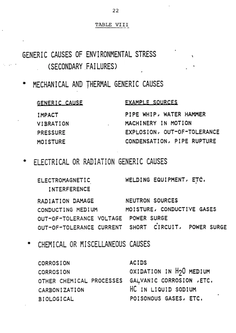
candidates, both for relative unavailability and as a function of the specific generic cause (see Table VIII). The total system

unavailability is also calculated. The uncertainty bounds are also provided, in that mean and median values are printed out, as well as with error factors so that 5% and 95% confidence bounds can be determined, both at the top event and individual cutset level.

(The uncertainty analysis capability of MOBB is discussed further in IFI.C of this report.)

(29)

OUTPUT

Common Cause Domains

System Logic Model: Fault Tree Basic Events: Failure Rates, Beta Factors, Locations, Susceptibilities & Rankings, Manufacturers. Common Cause Candidates Listing with Unavailability Generic Cause Listing System Unavailability Figure 3

Flow Diagram of MOBB Code

M 6 BB

_~_~I_~~1_I _/_1J_ n~~VLI________LI-~

INPUT

-~3

(30)

--TABLE VIII

GENERIC CAUSES OF ENVIRONMENTAL STRESS

(SECONDARY FAILURES)

MECHANICAL AND THERMAL GENERIC CAUSES

GENERIC CAUSE EXAMPLE SOURCES

IMPACT VIBRATION PRESSURE MOISTURE

* ELECTRICAL OR RADIATION

ELECTROMAGNETIC INTERFERENCE RADIATION DAMAGE PIPE WHIP, MACHINERY WATER HAMMER IN MOTION EXPLOSION, OUT-OF-TOLERANCE CONDENSATION,

GENERIC CAUSES

PIPE RUPTURE WELDING EQUIPMENT 1 NEUTRON SOURCES ETC.

CONDUCTING MEDIUM MOISTURE, CONDUCTIVE

OUT-OF-TOLERANCE VOLTAGE OUT-OF-TOLERANCE CURRENT

POWER SURGE

SHORT CIRCUIT, POWER SURGE

* CHEMICAL OR MISCELLANEOUS

CORROSION CORROSION

OTHER CHEMICAL PROCESSES

CARBON I ZATION BIOLOGICAL

CAUSES

ACIDS OXIDATION GALVANIC

HC

IN

H

₂

0

MEDIUM CORROSION ,ETC. IN LIQUID SODIUM GASES, ETC. GASES POISONOUS

(31)

B. Sample Problems

Two problems are performed below demonstrating the use of the MOBB code. The first demonstrates the ability of MOBB to evaluate and quantify individual system cutsets, while the second demonstrates that not all problems will require the full application of code capabilities (i.e.: in the second problem, one common

cause type dominates--human error). These examples demonstrate that utility system common cause analysis must still depend largely on the analyst's interpretation and understanding of the problem--no code can substitute for this basic requirement.

B.1. Warehouse Fire Protection System (FPS)

To demonstrate the use of the MOBB code, a sample problem has been devised based on a system for fire protection installed at a fictitious warehouse. (A similar system is used as an example

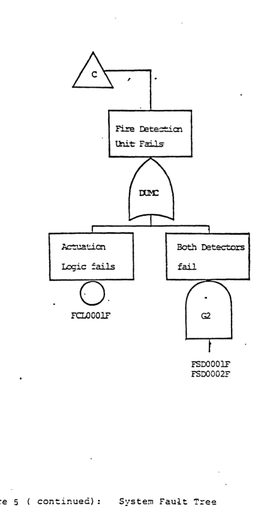
in Part IV.C of this report, the difference being that on- and off-site electric power is included in that example.) The schematic flow

diagram for the fire protection system (FPS) is shown in Figure 4. In Figure 5, the system fault tree is drawn.

In Figure 6, a sample floor map and suceptibility map is shown, whereby the code user must specify the relative location of the

components in his system and their geometrical susceptibility (i.e., across all compartments, only a few, or only one).

Then, the user must identify the particular failure mode of each component; in this case four modes are identified, as shown in Table IX. The susceptibility type must be specified for each domain, as shown in Table X, where "P" stands for generic cause or

(32)

Warehouse

(33)

I -XV001AC FCvOO02AC F"Zv'OO03 AC FXV0O4AD FPM:".OOLA ..0 0O1kF

=iue 5~: Syst an Fault Tree

25 I.,VOOJR0c C7002BC FXVIaOO33-C

FxvAo

W

4;F

0 02

BA F7,P.CO23?

(34)

FCLOI1F

FSD0001F

FSD002F

(35)

Floor MapD and Susceptibility Maps Floor Map YMAP - A MAP - B

.M.P - C

_1MIDC _2MPC _3MPC Al A2 A3 -igure 6:

(36)

Failure !Mode Code

S,-bol Failure Mode

C Closed

0 Open

A Fail to start

Fail to function

Table X : Susceptibi~ty Domain

Susceptibilitv Domain Physi ca! Location

P IMPA Al, A2, A3

1, V, T 1MPB Al 2 LPB A.2, A3 G, M, C, 0 ILMPC Al 2MPC A2 3MPC A3 Table

LX

:

(37)

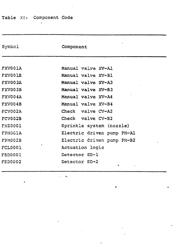
susceptibility to pressure, "T" for temperature, "V" for vibration, etc. Then,each component in the system must be labelled for

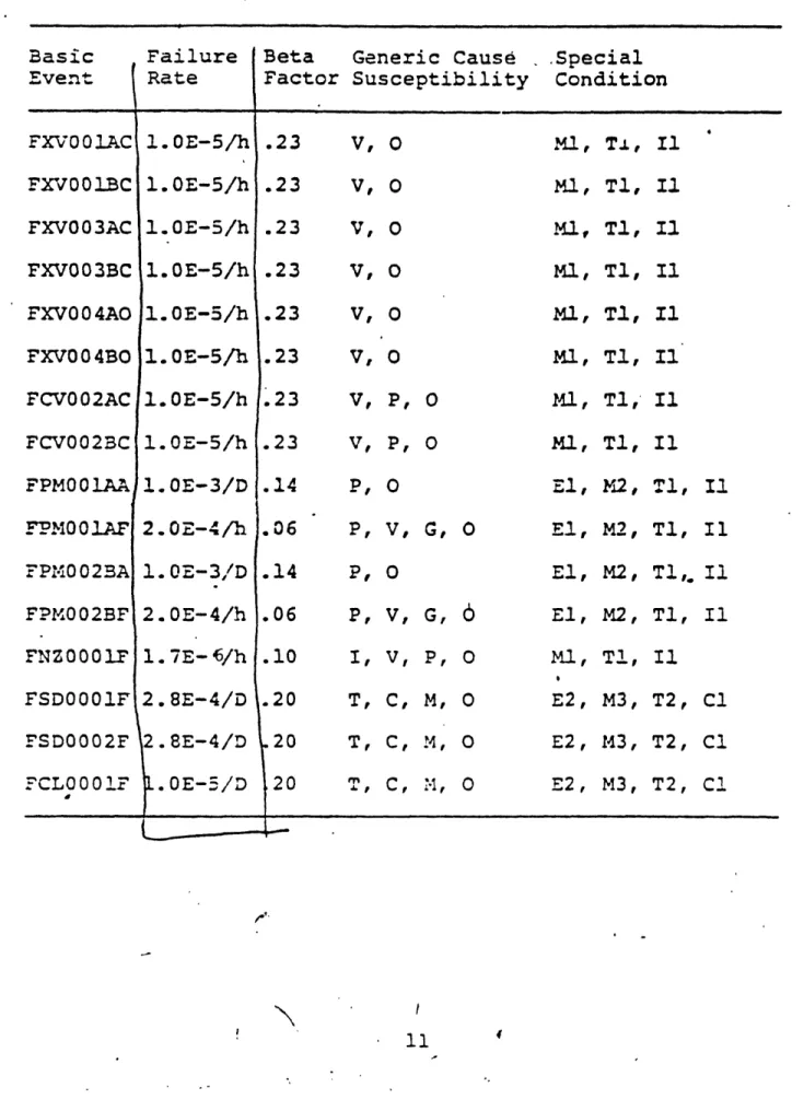
input into the code by type, number, and failure mode (Table XI). Finally, the common cause failure data and total component failure

rates, either input on a per hour or per demand basis, must be defined, as shown in Table XII.

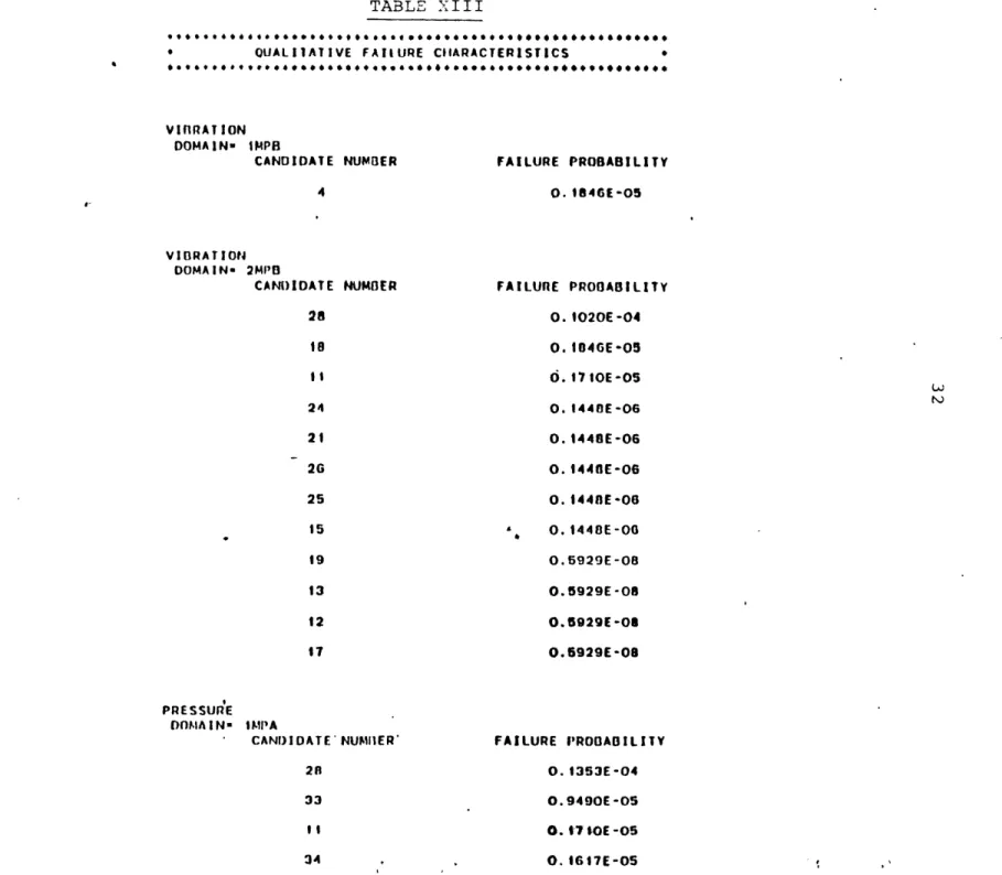
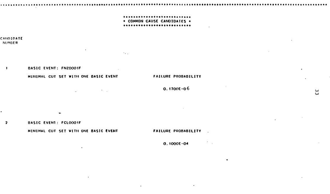
Results of running the MOBB code for this sample problem revealed thirty-four common cause candidates (See Tables XIII - XV; sample

computer output) which include two cutsets with only one component. Strictly speaking, they cannot be defined as common cause candidates, but are included because they are significant contributors to

the total system failure. The system failure probability due to independent failure is estimated at 1.21E-4 and the failure proba-bility due to common cause failure is 4.12E-4 (i.e. system failure due to common cause is three times as high as failure due to random

failures). The total system failure probability is 5.33E-4 compared to the original single pumping train system which has a failure

probability of 3.4E-3. There is almost an order of magnitude improvement in decreasing system unavailability.

If the assumption of total statistical independence of components is valid, the system unavailability can be as low as 1.OE-5 (the

single component cutsets are dominant contributors). On the other

hand, if the failure is totally dependent, there will be no improvement by adding an additional train to the FPS. In practice, the result

often attains some value between these two extremes.

(38)

~-_lliiLI-~--Table XI: Component Code Component FXVO 001A FXV001B FXV003A FXV003B FXV004A FXV004B .FCV002A FCV002B FNZ0001 FPMO G IA FPM002B FCL0001 FSD0001 FSD0002

Manual valve XV-A. Manual valve XV-Bl

Manual valve XV-A3 Manual' valve XV-B3

Manual valve XV-A4 Manual valve XV-B4 Check valve CV-A2 Check valve CV-B2

Sprinkle system (nozzle) Electric driven pump PM-Al

Electric driven pump PM-B2 Actuation logic

Detector SD-1 Detector SD-2

Symbol 1

(39)

31

Table XII: Co~mon Cause Failure Data

Basic Failure Beta Generic Cause .Special Event Rate Factor Susceptibility Condition

FXVOO1AC 1.0E-5/h .23 V, O MI, T, Il FXV001BC 1.OE-5/h .23 V, 0 MI, Ti, Ii FXV003AC 1.OE-5/h .23 V, 0 MI, TI, Ii FXV003BC 1.0E-5/h .23 V, O Ml, TI, Ii FXV004AO 1.OE-5/h .23 V, 0 MI, TI, Ii FXV004BO 1.OE-5/h .23 V, 0 Ml, TI, II FCV002AC 1.OE-5/h .23 V, P, 0 MI, TI, II FCV002BC 1.0E-5/h .23 V, P, O MI, TI, Il FPMOO1AA 1.0E-3/D .14 P, 0 El, M2, TI, Ii FPM001AF 2.0E-4/h .06 P, V, G, 0 El, M2, TI, Il FPM002BA 1.0E-3/D .14 P, 0 El, M2, T1,. I1 FPM002BF 2.OE-4/h .06 P, V, G,

6

El, M2, TI, Il FNZ0001F 1.7E-6/h .10 I, V, P, O MI, Tl, Il FSD0001F 2.8E-4/D .20 T, C, M, 0 E2, M3, T2, Cl

FSD0002F 2.8E-4/D 120 T, C, M, O E2, M3, T2, Cl FCL0001 .0E-5/D 20 T, C, M, 0 E2, M3, T2, CI

(40)

I1I I CM ltl itd CALISF All 1:C AIJAI VSIS FOn FIRE PR)TEC/ SYSTMF1 O(B1 P L I 1 u 14 lI(UN. I StW:l E P1lOl.EM FOR iMOAUE2

Sc 20

MOBABE 2 - VERSION 2 SE rtuil11/lln

TABLE XIII

* QOUALilATIVE FAIlURE CIARACTERISTICS

* ,***** c4e*** 0 * *, **s#*, e .***.*******## **** VIIRAT ION DOMAINu IMPB CANDIDATE NUMBER 4 VIBRATION DOMAIN- 2MI'B CANDIDATE 28 18 II 24 FAILURE PROBABILITY 0. 84GE-05 NUMBER PRESSURE DOMAIN= IMPAA CANDI)DATE NUMIIER" 28 33 II 34 , FAILURE PROOABILITY 0.1020E-04 0.1046E-05 0. 17tOE-OS 0.1440E-06 0.1440E-06 0.1446E-06 0.144LE-06 0.1448E-00 0.5929E-08 0.5929E-08 0.5929E-08 0.6929E-08 FAILURE PROBABILITY 0.1353E-04 0.9490E-05 0.t tOE-05 0.1617E-OS

(41)

i I it COMMONr CAIJSI

,I( , 111t S liA l 1 1 O3

fAllt Ifr AIJALYSIS FOl FIRE i'POTECTf SYSTEMI

SAM1'I.I Ii(l1l I 14 I O l )l AIIE2

I5 2 - v. 2

M0flAftE 2 - VtIlS1(lfl 2 . 11 mill II/n I

TABLE XIV

OUIPUT FROM MOIIABE 11

* COMMON CAUSE CANDIDATES * e*eeoeeoeeeeee ee eeee~eoee

CANDIATE

NUMB ER

BASIC EVENT: FNZOOOIF

MINIMAL CUT SET WITIH ONE BASIC EVENT FAILURE PROBABILITY

0. 1700E-06

BASIC EVENI : FCLOOOIF

MINIMAL CUT SET WITH ONE BASIC EVENT FAILURE PROBABILITY

(42)

it r: COMMlON CAUSF I All II[ ANAI.YSIS FOI F IRE PROTECTIOh .STEit

10t: SA 't r rRnnfLrM FOR MOIABE2

*,'.: 0

I)+1iiiri , I, VI sw11 i srtr*imH0l p/n I

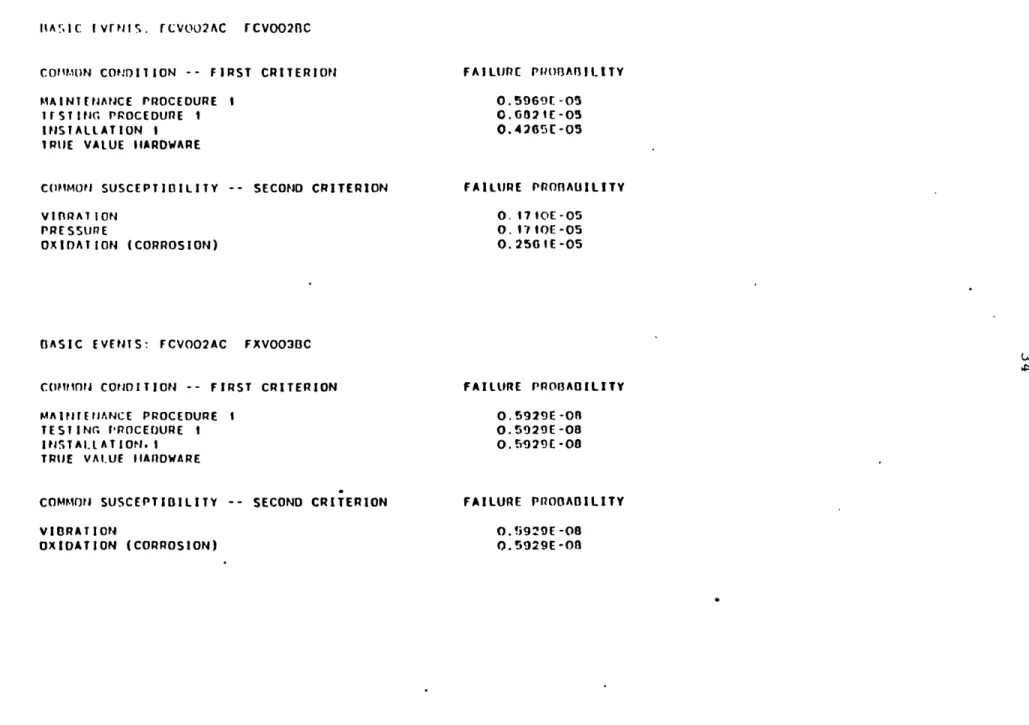
TABLE XV

IIA'IC IvrNIS. rCVOO2AC rCVOO2nC

COM .ON CONDITION -- FIRST CRITERION

MAINTENANCE PROCEDURE I

IFSTING PROCEDURE I

INSTALLATION I

IRUE VALUE IIARDWARE

C(IIMMON SUSCEPTII31LITY -- SECOND CRITERION

VISRA1 ION PRESSURE OXIDATION (CORROSION) FAILUnE P1oIAB!ILI TY 0.5969 -05 0.602 E-5O 0.4265E-05 FAILURE PRO3AUILITY 0. 7 tOE-OS 0.1710E-05 0.250 1E-05

1ASIC EVENTS: FCVOO2AC FXVOO3BC

C(o MfIn CONDITION -- FIRST CRITERION

MAINTfE1IANCE PROCEDURE I

TESTIN I'PROCEDURE I

INSTAILL ATION. I

TRUE VAI.UE IIARDWARE

COMMON SUSCEPTIBILITY -- SECOND CRITERION

VIBRATION OXIDATION (CORROSION) FAILURE PRAOABILITY 0.5929E-OR 0.5929E-08 0.5929 -00 FAILURE PROOABILITY 0.9929E-08 0.5929E-08 010 tll lI

(43)

35

B.2 Millstone-I Automatic Pressure Relief (APR) System

A sample problem was analyzed for dominant common cause con-tributors. The system analyzed was the Millstone-I APR (automatic pressure relief system). A description of the system and the fault tree for that system are given-in Appendices C and D. It was

found that human error dominates, so that the MOBB code was not

fully applied to run this problem. Results are shown in Figures 7 and 8. C. Propagation of Uncertainty in MOBB

The MOBB code (20) was modified (as shown in Tables XVI-XVII) to compare the Monte Carlo simulation method for propagating component failure rate uncertainties through the fault tree as compared to

the more analytic Method-of-Moments. This was done to establish a distribution on cutset availability rather than printing only a single point-value.

It was found that the Method-of-Moments was by far the more efficient of the two approaches. Improvements on the Method-of Moments were made by using modified lognormal distributions to model component failure rates. These are termed, "S", for the

standard lognormal, "SB" for the bounded lognormal, and "St" for the truncated lognormal. The mathematical formulae for each is given in Table XVIII,with behavior of the functions shown in Figure 9. The bounded lognormal, S B was found to render the best results on a sample problem taken from a recent reference,* where results

agreed well with a Monte Carlo simulation of 3,000 trials (Table X1X). The Method-of-Moments was therefcre implemented with the Sb approximation.

Work done at Westinghouse.

(44)

Figure 7

Fault Tree for APR System for Human Error

APR Auto-Remote Actuation Mode Failed due to Human

Error

Sensor

Operator resets APR actuation logic during accident

I

C

A B A B A B

A: not restored to service after test or maintenance B: switch or sensor miscalibrated

(45)

Figure 8

APR System Analysis 1) Blowdown for LPCI systems

Scenario: small LOCA

Success Criteria: 2 out of 4 Auto/Remote APR Valves actuate

APR System Fails to Depressurize the System

3/4

APR-3A APR-3D APR-3C APR-3F

2) Relief/Safety Valves Actuation

Function:to relieve high vessel pressure Full Power Pressure: 1,000 psig

Design Limit Pressure: 1,375 psig

Success Criteria: Any 4 out of the 6 APR or R/S Valves Scenario: -Turbine Trip from Full Power

-Failure of the Turbine Bypass System -Failure of the Direct Reactor Scram

based on Stop Valve Position

R/S Valves Fail to Reduce Vessel High Pressure

3/6

APR 3A APR-3D APR-3C APR-3F S/R-3B S/R-3E

3) Manual Actuation Mode

All six valves can be remotely opened from the control room Success criteria: -Relief Pressure 4/6

-Blowdown (auto/remote) 2/4 -Blowdown (manual) 2/6

(46)

38

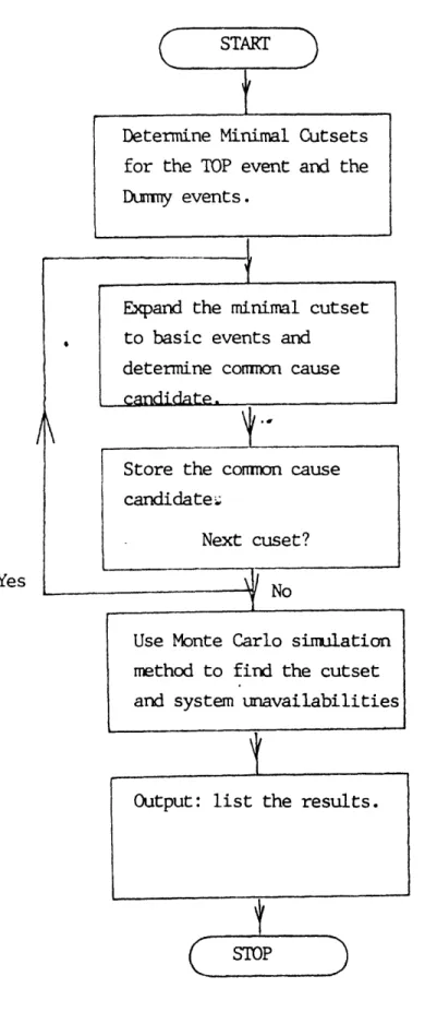
TABLE XVI

MOBB WITH MONTE CARLO

START

Determine Minimal Cutsets for the TOP event and the Dummy events.

Expand the minimal cutset to basic events and determine common cause

Store the common cause candidate.

Next cuset?

No

Use Monte Carlo simulation method to find the cutset

and system unavailabilities

Output: list the results.

STOP Yes

(47)

39 TABLE XVII

MOBB WITH METHOD OF MOMENTS

START

Determine Minimal Cutsets for the TOP event and the dumny events.

Expand minimal cutset to basic events and check

for comnon cause/comon link failure.

-Calculate the cutset unavailability using the method of moments.

Yes Next Cutset?

No

Calculate system unavail-ability from the means & variances of the cutsets.

lStop

I~""-Llr*iWYIIP(LsEmnti~Ewn~-*ir~mb^..~- ;i-ii~uwrri~rr

(48)

TABLE XVIII

MATHEMATICAL FORMULAE FOR VARIOUS LOGNORMAL FUNCTIONS EMPLOYED IN METHOD OF MOMENTS

Log-normal Probability Distribution S1(xl p,o)

S₁(XI ,a) xa/2a 0 0 <x < otherwise mth Moment = exp[mp + m2a 2/2 ]

Bounded Log-normal Probability Distribution Sb(xip ,o)

Sb(Xl,a) = 1 exp[(log( l--x 2/(-2 2) x(l-x)o/J2Tr 0<x<l1 =0 mth Moment = 10 x Sb(xlp,a) dx otherwise

Truncated Log-normal Probability Distribution S (xh i,o)

S (xlp,a) = , xov/2

exp[(log(x)-P)2_/(-22)]

=0

where C is the normalization factor

C = f0 Sl(xjp,o) dx

mth Moment = 1O x S (xlp,) ₀ _t dx

0 <x<1

otherwise exp[(log(x)-P)2/(-22)]

(49)

Figure 9

Behavior of Various Lognormal Function Options

Log {mth Moment) Log0{ 0 m x f(xlp,a)dx} _6(m,p,a) St(XIV,o) Sb(XI ,o) f0 x Sb(xlj,oa)dx- fo xm S1(xl,,o)dxl ) xm Sb(xlo,)dxl Im 0 x S (xp,)dx -S(0 xI S(xp,),o)ddxx x 10 x MS (xx , )dxl1 Log (m)*

_~.~....~~,.;4--r-ii--~--l~^-^~ap~ --i----I rl-(- II L-1'I-YIL~^I~- (OI^-IUC-I-I~-I~

___

6(m,P,G) =

(50)

TABLE XIX

SAMPLE UNAVAILABILITY EXPRESSION: RESULTS OF COMPARISON

Boolean Expression for system unavailability: S = X, + X₂X₃+ X₄X5 + X6

Basic Events Median of failure probabilities

X1 1x10-3 X₂ 3x10-2 X₃ 1x10-2 -2 X₄ 3x10- 2 X5 1x10-2 X₆ 3x10-3 RF=3 RF=10

Method Mean Variance Mean Variance

Discrete 5.936x10- 3 7.2x10- 6 1.49x10-2 2.14x10-4 Method of Moments: S1 5.936x10-3 9.4x10- 6 1.491x0-2 8.76x10- 4 Sb 5.933x10-3 9.4x10-6 1.410x10-2 3.97x10-4 St 5.938x10- 3 9.4x10-6 1.424x10- 2 4.80x10-4 Monte Carlo Sample (3000) 5.955x10-3 8.6x10- 6 1.426x10-2 3.97x10 Sample (1200) 5.996x10-3 9.3x10- 6 1.477x10-2 4.73x10-4 Discrete -3 - 6 1.402x10-2 _1.89x10-4 (1200) 5.788x10 6.3x10 1.402x10 1.89x10

(51)

Even so, the differences seem relatively minor when plotted

(Figure 10); yet the Sb approximation appears easier to implement

for numerical calculation reasons, and is most accurate. Nevertheless, any choice involving the use of the Method-of-Moments is more

efficient than Monte Carlo simulation; a factor of at least

10 in savings in computation time can be expected based on this project's experience in running the code.* Supporting material

is provided in Appendices A-B of this report.

IV. Cutset Susceptibility Concept for Common Cause Analysis A separate analysis technique for analyzing common cause failures was applied in this project, with results compared to that of MOBB for treating cutset uncertainty. A simple code for performing discrete probability distribution (DPD) arithmetic was developed and applied to a sample problem, that of the warehouse fire protection system (FPS) analyzed earlier (see section

B.1), but this time, for seismic contribution to total system un-availability. Finally, a comparison of uncertainty treatment is made with that of the MOBB code.**

A. Method Description

As described in section II.A: "Dependent Failure Analysis", so-called "external" events, such as earthquakes, floods, and fires, are a type of dependent failure or common cause failure

mechanism. The method which has been developed to deal with seismic

*This result supports the finding of Jackson and Lee, et. al.

r21)

and Bier 22).

**This work would be more fully developed in the follow-up proposal for next year (see Appendix F.4 for proposal description.

(52)

I *E LOC3ART~ikiC -, o " CvC-ES_{LO~Ae,, iM} _,_-_CCE _4E_7;22

Figure 13

Plot of Resulting Curves of Top Event Unavai--abiity

PDF(x) 1 2 3 A 6 7 Ej;1 1 o 3 4 789 -5 -4 -3 2 3 4 5 6 789 -2 10 2 3 4 56 : 10 : 1. 10 102 1 2 3 5 6 7 8 - ' _,_; - _ _._{... .. .., , i}:-~- • )-_T _- _- _,, ,-T . i_- T-- r-7-i- -~ ... '- -- 1- ' , T IT I : ; i t ....--- I , I- ; ." i 10~~___

_IjI

_{I- --TS}_br.~.L

i2 it

S"

f

_..

_{. - ..,}

_----

₀

_)...

S _ -' -; -actor :10 101 '. i i I -; -I "i i i ! 4 ' :YU'1I -h " -...

i

' , "

ii

f t

i

',

_{, '}

_'

i

_.)

_'...

_{" . .}

_.

j~~~~~~- I T-: : iMdr r\ ~I;~T 2• i

t

__, , ,.. I. . , 'j. f: 't. * . I. 4 .' . 7---'.. :111 i .jjl: 11 it'I !jL F - . . . . .. . ,- t ... , ;- i- 111; 1%- 11V -J!J 1!! 1" . . .. II f ' Ii l o "o it 1

l

" ,

,

I

(

_I!

:

:_

.:

_i"

i

_{I:: i.}

i

_...

:,,:1.

_i

1.0:.! tj 4

.tIi ijf:i - ~ I 'Iijir:

1lL-.... .... ... . .... ... ' .... ' t i ' ...i ,- ... , _ i .. ~ _..i t L r! ::: 1ri I :,lll: (- , .1 I i . ; . .

-1:

"4 : iii~ll • :

. .L .j_

' "

::

lli ii Ilt! ! t l i .if , 1l 1!14 S .... .I 11i I iiji " H-10- 5 10 - 4 10- 3 10- 2 10 -1 1.0

(53)

risk quantification in nuclear plant risk assessments can, in fact, be applied to quantify other dependent failure mechanisms of the "internal" type (i.e., humidity, pressure, temperature, vibration, human error, etc.). The only constraint in the application is that due to data collection, yet the seismic risk methodology allows for a clear presentation of the data uncertainty that perhaps makes it a more preferable approach to other methods.

The basic idea would be to identify all system cutsets that

are common cause candidates, thus first employing the MOCUS-BACFIRE II packagp, and then substitute for the Beta-Factor CCF quantification package with the separate code developed here employing the seismic risk method approach. The mathematical details of the approach are now described.

A.l. Treatment of Uncertainty Using DPD Arithmetic (from PLG Handbook, ref. (2))

In calculations of real world phenomena, there is almost invari-ably significant uncertainty in the numerical values of parameters.

In these calculations, numerical quantities can be replaced by probability distributions and mathematical operations between

these quantities should be replaced by analogous operations between probability distributions.

in risk and reliability calculations, it is often necessary to perform various operations between probability or frequency distributions. Take the example of a simple series system of

two components with failure rates X1 and X2. Then the system failure rate, X, can be defined as:

(54)

If we express our state-of-knowledge about the component failure rates with probability density functions, Pi(Ai), then the

probability distribution for A is the sum:

S

Ps( s) = P₁(X₁) + P₂(X₂) (19)

where the symbol "+" between two distributions is understood to stand for the convolution operation:

Ps(As) = P 1 ( 1 )P 2 (As-Ai)dA1 (20)

0

assuming states-of-information P₁ and P2 are independent.

For a parallel system:

A =1 x 2 (21)

Ps(As) =P 1(A 1) x P2( 2) (22)

where "x" corresponds to the multiplicative convolution operation:

P ( P (A)P X ) dX 1 (23)

s s 1 1 2 A1

1 1

0

Combinations far more complicated than this occur routinely in risk and reliability work. Usually, Monte Carlo can be used to compute these combinations. An alternate approach is the method of discrete probability distributions (DPDs).

(55)

Rules of DPD Arithmetic

Let X be an ordinary scalar variable, and let X1, X2 ... Xn

denote particular discrete values of x.

Let P 1 P2 ... Pn be the associated probability values such that:

n

P ₁ =

Then the set of doublets

<Pi X>' <P2' X2> .."'. <P, Xn > = <Pi ' X.>

is the DPD and is an approximation to a continuous pdf.

'--.

.j1

a I I a. I

I

a-)

k

-1,

Probabilistic Addition

Suppose Z = X + y, x = _{<Pi' X} I Y = <qi' Yi > (26) Suppose X and y are independent (they are based on independent states of information: Then Z = <P., ₁ X.>₁ + <qj, yi> _j ₁ (27) = <Pi.qj X + Yi> (28) this DPD represents our state-of-knowledge on Z (29) - <rij Z..> (24) (25) -rli.*--n^-iuuu.-rri l u~- ~l --- r~^;~ -~4*~-~~CF-- r*"

-f

-

Ns.,

(56)

48 where raj = Pq, Z.. = X. + y j (30) Example: X =<.1,-1> <.5,1> <.4, 2> ₍₃₁₎ y = <.2,5> <.8,10> (32) Z = i<.0 2,4 <.1,6> <.08,7> <.08,9> <.4,11> <.32,12>3 ₍₃₃₎ S<Piqj , X. + yj> Multiplication i ,X >* b c, y >3 = <Pjqj X y >3 (34) Functional Definitions

Consider Z = f(X), X = <Pi, X.i (35)

so Z = <Pi,f(X i)> (36)

We enter the curve

t

f(X) with a probability

distribution for X and emerge with a distribution for Z.

Suppose now that f itself is also probabilistic (there is uncertainty on f). _{We can express quantitatively this uncertainty} by setting out a series of different functional forms f. and

I assigning probabilities to each:

f = <qj,f>3 _; _C_{qj = i.}

j (37)

Graphically:

We enter a probabilistic

function with a probabilistic argument and emerge with a probabilistic output. If both X and f are probabilistic, then

(57)

49

z

j,

] i

f is plotted as a "band"--a family of curves with P as a parameter. Pitfalls

1. Nondistributivity of Probabilistic Operations In ordinary arithmetic, if

Q = X[y+Z] then

Q = Xy + XZ distributivity

This does not hold for DPDs--pay careful attention to the sequencing of operations.

2. Independence and Dependence

Suppose Z = 2X: X = <.2,1><.6,2><.2,3>i Then Z = <.2,2><.6,4>,<.2,6> Suppose Z = X + X

Then Z = .04,27><.24,3><.44,4><.24,5><.04,61> Thus Z = 2X / Z = X + X. The difference is that when we did the operation X + X, we treated the two distributions as if they were independent. THEY ARE NOT. Thus, we obtained compensating uncertainties and a more narrow distribution than we should have. This situation arises particularly in risk calculations between similar components.

Thus, use A_s= 2X1 for series system when components are identical

(not As = 1 +X ₁)

2

and s = 1 for parallel system

(not _s =A _{1 1}x 1)

(58)

50

A.2 Application of Method to Seismic Risk Calculations (2)

Suppose we have a specific structure, S, at a specific location, L, and wish to know the risk of collapse of this structure due to earthquake.

What we use is a "seismicity" curve and a "fragility" curve, as follows:

Seismicity Curve Fragility Curve

I.0 -a)

F

&El

k-e er4"j' ,)C PeA AcCeierat o X&

Assume that we run the experiment and knew the curve F(a) exactly. Suppose also that we had monitored the site L for millions of years and knew the curve 0(a) exactly.

The frequency of structural failure due to earthquake would be given by:

( = - d f(a)da

(39)

0

Probabilistic Calculation

We really do not know the seismicity curve 4(a) exactly. Therefore, using the DPD idea, let us express our uncertainty in

4(a) by putting forth a finite family of curves, Di(a), and assigning to each a probability Pi:

(59)

51

Thus:

S E <P i,(a)> (40)

or graphically:

0-We also do not know the fragility curve exactly, so we express our state-of-knowledge about the fragility by writing a DPD:

F <qj, Fj(a)> (41)

1.01(

0-Now, we perform the operation

f = - - F(a)da (42) 0 using DPD arithmetic: f = I<PijP. ij,> (43) where Pij = Piq. (44) and = (d i ) F.(a)da (45) ij da

(60)

This is the "Probability of Failure Frequency" idea.

B. Code Description

The method described in section (A) has been extended as follows to analyze "internal" common cause events. For each

location in the plant, an "environmental stress" curve analagous to the seismicity curve in seismic risk analysis is defined by

the user (see Figure 11). A family of such curves can be specified for the 95%, 50% and 5% confidence levels reflecting the analyst's uncertainty about the function 4(X).

Next, the susceptibility of the cutset must be specified, again as a family of curves. This curve can be synthesized from knowledge concerning the individual component susceptibilities to each stress type, or on a multi-component, or cutset, level depen-ding on the analyst's choice (see Figure 12). This curve must be defined as a function of whether one considers the system to be operating under normal or accident conditions, where "A" refers to

the conditions considered (A1 for "normal"; A2 for "accident") and

to the state-of-knowledge of the analyst who is specifying this curve. The result of the analysis are probability density functions,

or PDFs, about the frequency of failure (or unavailability) for each cutset as a function of the particular environmental stress

(61)

53

Figure 11

Environmental Stress Curve*

Frequency (yrs -1)

(at location L)

ss X

Analogous to seismicity curve.

Figure 12

Cutset (Component) Environmental Susceptibility Curves*

.

F -Failure Fraction --Stress level X Fj(X) = ability of cutset j to resist various levels of environ-mental stress X.

Analogous to seismic fragility curves.

Figure 13

Result of Environmental Stress Analysis on System Cutsets

Probability Density

I

(j

4

,i;JZ

1 3-

4 t4

332

Failure Frequency

(62)

Tlis _{method then produces a probability distLibutionl on} _each cutset's unavailability, indicating uncertainties. The Boolean expression for the top event is then used,which will generally

be just the sum of all the cutsets, so that the total system unavail-ability may also be expressed as a "probunavail-ability of frequency"

distribution.

Implementation of the actual calculational procedure employed in this approach is shown in Table XX.

C. Sample Problem: Warehouse FPS

The warehouse FPS of section III.B.1 was analyzed here for failure susceptibility to seismic events using the DPD code written in this project. _{The FPS was analyzed for three cases (see Figure 14):}

Sl -- one pump train only (PTB) and no diesel generator

S2 -- _{one pump train with both diesel generator and off-site} power

S3 -- _{both pump trains with both diesel generator and off-site} power

The fault tree for each of the three system definitions was drawn (Figure 15) and the Boolean expression found for the top event

(see Table XXIfor System S3). _{Assumptions were made on the relative} fragility of each cutset to seismic events (see Figures 16-22). The seismicity of the site was taken to be that of the Zion nuclear plant

side in Chicago for representative purposes only (Figure 23).

Final results of the example calculations are shown in Fiqure 24 indicating the uncertainty of each cutset unavailability due to seismic events. Note that Sl has a median failure probability

(63)

TABLE XX

CUTSET FRAGILITY CONCEPT APPLIED TO ANALYZE CCF

Define Common Initiating event frequency of occurrence. Define cutset's conditional susceptibility functions. Compute cutset unavailabilities due to that common initiating event.

Yes Next cutset

no

Compute system unavaila-bility due to that common initiating event using the DPD method. Next yes common initiatiny event? j _Y_ rlC~I^___II1^I_111*-_)*--_

(64)

11~---Fiqure 14

Modified Warehouse FPS with Added Diesel Generator

(65)

57

Figure 15

System Fault Tree (Sheet 1 of 3)