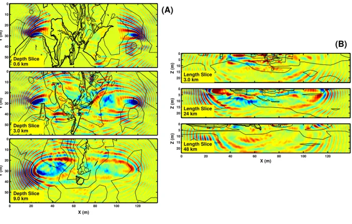
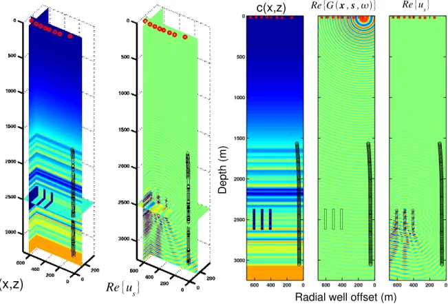
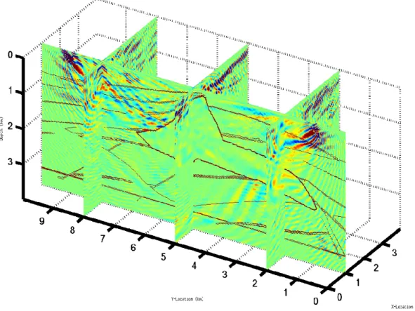
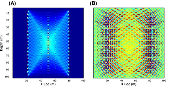
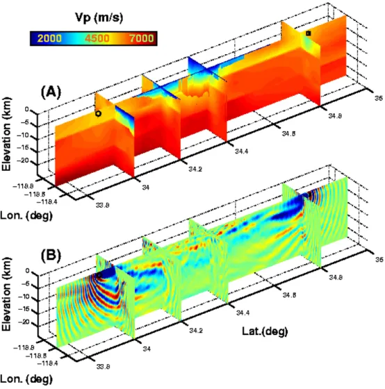
Computation of 3D Frequency-Domain Waveform Kernals for c(x,y,z) Media

i) We need two image charges, one for each one of the real charges producing the constant external electric field.. The first term is just the potential due to the external field

Abstract—In this paper, we propose a successive convex approximation framework for sparse optimization where the nonsmooth regularization function in the objective function is

Proposition Une matrice A (resp. un endomorphisme u d’un espace de di- mension finie E) est diagonalisable si et seulement si il existe un poly- nôme annulateur de A (resp.

Conversely, it is easy to check that the latter condition implies that T a is bounded.. Moreover Λ is composed of eigenvalues λ associated with finite dimensional vector

In this thesis, with the assumption of infinite depth water, heave added mass and damping coefficients of a floating hemisphere, a Wigley hull and a Liquefied Natural

Ex- periments on the MusDB dataset show that, with proper data augmentation, Demucs beats all existing state-of-the-art architectures, including Conv-Tasnet, with 6.3 SDR on

TFM has topological (connectedness, closure, neighborhood, and continuous mapping) and functional (cause-effect relations, cycle structure, and inputs and outputs) characteristics.

Despite analyzing the global processing sequence (Fig. 12, right) by feeding the signal processing chain with a synthetic signal spanning from 0.05 times the sampling rate to 0.4