Capacity of and Coding for Multiple-Aperture, Wireless, Optical Communications

(1)

Capacity of and Coding for Multiple-Aperture,

Wireless, Optical Communications

by

Shane M. Haas

B.S. Mathematics, University of Kansas (1998)

B.S. Electrical Engineering, University of Kansas (1998)

M.S. Electrical Engineering, University of Kansas (1999)

M.A. Mathematics, University of Kansas (1999)

Submitted to the Department of Electrical Engineering and Computer

Science

in partial fulfillment of the requirements for the degree of

Doctor of Philosophy in Electrical Engineering

at the

MASSACHUSETTS INSTITUTE OF TECHNOLOGY

May 2003

c

° Massachusetts Institute of Technology 2003. All rights reserved.

Author . . . .

Department of Electrical Engineering and Computer Science

May 14, 2003

Certified by . . . .

Jeffrey H. Shapiro

Julius A. Stratton Professor of Electrical Engineering

Thesis Supervisor

Accepted by . . . .

Arthur C. Smith

Chairman, Department Committee on Graduate Students

(2)

(3)

Capacity of and Coding for Multiple-Aperture, Wireless,

Optical Communications

by

Shane M. Haas

Submitted to the Department of Electrical Engineering and Computer Science on May 14, 2003, in partial fulfillment of the

requirements for the degree of

Doctor of Philosophy in Electrical Engineering

Abstract

Refractive index turbulence causes random power fluctuations in optical communi-cation systems, making communicommuni-cation through the atmosphere difficult. This same phenomenon makes the stars twinkle at night, and pavement shimmer on a hot sum-mer day. True to the old adage, “don’t put all your eggs in one basket,” we examine laser communication systems that use multiple transmit and receive apertures. These apertures provide redundant replicas of the transmitted message to the receiver, each corrupted separately by the atmosphere. Reliable communication occurs when not all of these paths are deeply faded. We quantify the maximum rate of reliable com-munication, or capacity, and study space-time coding techniques for both direct- and coherent-detection receivers. We also experimentally verify the performance of some simple techniques for optically-preamplified, direct-detection receivers.

Thesis Supervisor: Jeffrey H. Shapiro

(4)

(5)

(6)

(7)

Acknowledgments

I would like to foremost thank my research advisor Jeff Shapiro. This thesis would not have been possible without his guidance and support. I am continually amazed at how he juggles being R.L.E. director, teaching classes, and still meeting every week individually with all of his graduate students. I have learned so much from him during these past four years.

I would like to thank my thesis committee member and academic advisor Dave Forney. He really helped me with my transition to M.I.T. Every semester, he would talk with me, and give me great advice on classes, career paths, and life. He also was a mentor to so many students, including myself, during the Area I Graduate Seminars.

I also want to thank Vahid Tarokh. Our discussions on space-time codes and information theory greatly influenced the development of this thesis. He also served as a member on my thesis committee.

For his help with the experimental aspect of this thesis, I would like to thank Franco Wong. In addition to his laboratory expertise, I really appreciated our con-versations about investing. Someday, I hope to convince him that derivatives are not evil. I also thank Baris Erkmen, Etty Shin, and Mohsen Razavi for helping with the experimental setup.

I would like to thank my officemate Chris Kuklewicz for our many enjoyable conversations. I am also honored to have introduced Chris to the fine beverage of Guinness.

My family and friends have always given me great support and encouragement. I want to thank my mother Judy, and my brothers Brett and Ty for being there for me during all of these years. I also want to thank Lillian for the time that we have spent together, and for the more to come.

Finally, I thank the Defense Advanced Research Projects Agency for supporting this research in part through grant MDA972-00-1-0012.

(8)

(9)

List of Figures

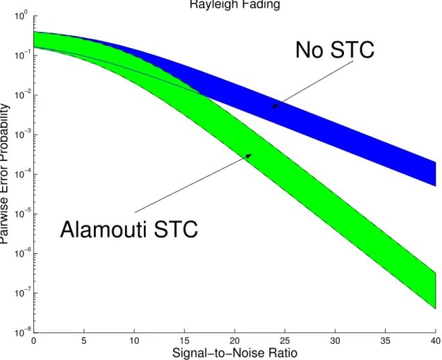
1-1 Space-time codes can improve the reliability of communication on fad-ing channels. The shaded areas lie between upper and lower bounds on the pairwise error probability achieved in Rayleigh fading with and without an Alamouti space-time code. The bounds are plotted as a function of signal-to-noise ratio. In this case, the signal-to-noise ratio is the ratio of transmitted codeword energy difference to the receiver noise variance per real dimension. . . 33 1-2 The pairwise error probability in moderate (σ2χ = 0.1) lognormal

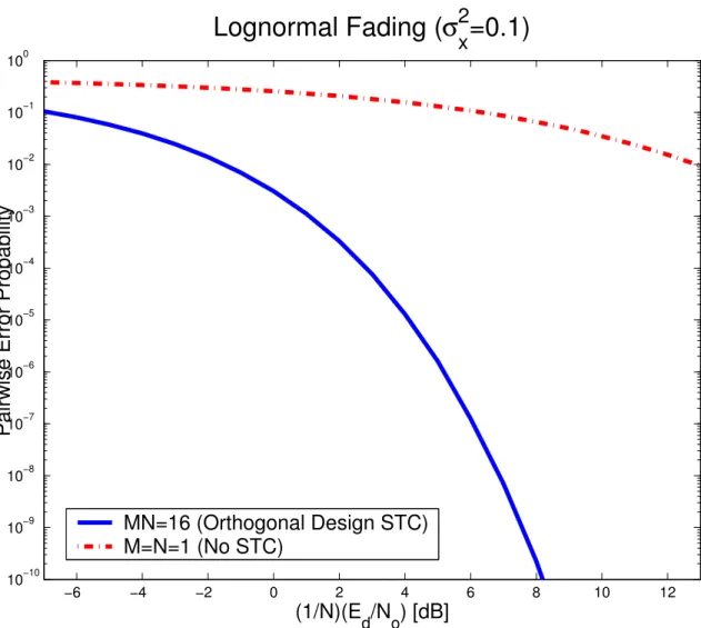
fad-ing is shown for an orthogonal design STC usfad-ing coherent detection receivers. The product of transmit (N ) and receive (M ) aperture num-bers is M N = 16. The error probability is plotted against the ratio of energy difference between codewords at the transmitter (Ed) per transmit aperture (N ) and receiver noise power spectral density (N0). Also shown is the single transmit, single receive aperture (M = N = 1) error probability when no space-time code is used. . . 34 1-3 Providing the receiver with multiple copies of the transmitted message

can improve the reliability of communication. This thesis explores the capacity of and coding for this multiple-input, multiple-output (MIMO) fading channel. . . 35

2-1 A modern optical communication system modulates a laser to convey information through a medium to a receiver. The receiver decodes the detected light and attempts to reconstruct the transmitted message. . 46

(14)

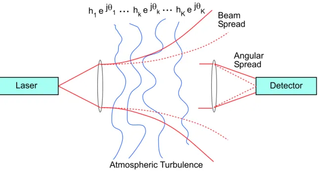
2-2 Light propagating through thin slabs of clear, turbulent atmosphere experience random amplitude and phase fluctuations. The cumulative effect of these variations is approximately lognormal in distribution due to the central limit theorem. Scattering also causes spreading of the transmitted beam, and an apparent increase in the angular extent of the source at the receiver. . . 48

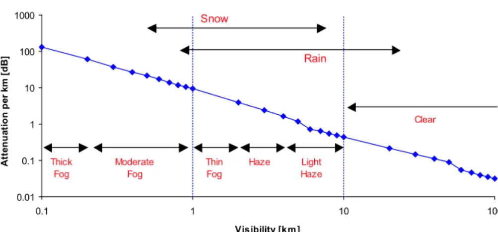
2-3 Mie scattering can cause an irretrievable loss in optical power. This figure shows the atmospheric power-attenuation per kilometer at the 1550 nm wavelength for a variety of visibility and weather conditions. For example, in clear weather, the visibility is greater than 10 km, and attenuation is less than one decibel per kilometer. . . 50

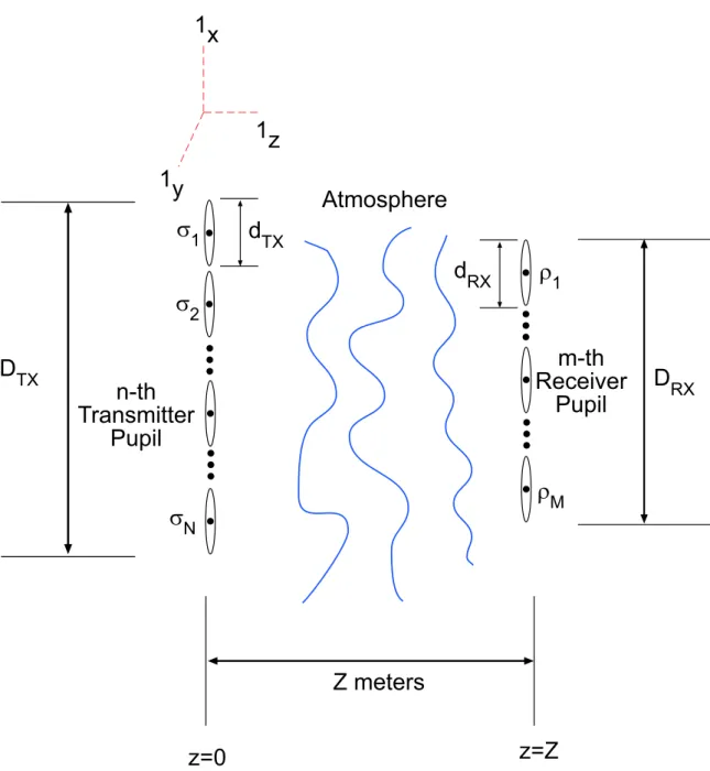
2-4 The geometry for the extended Huygens-Fresnel principle consists of the n-th transmitter pupil located at σn in the z = 0 plane and the m-th receiver pupil located at ρm in the z = Z plane. In this diagram, 1x, 1y, and 1z are unit vectors marking the origin. . . 54

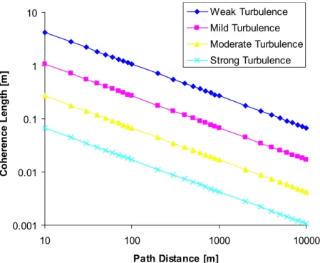
2-5 This figure plots the atmospheric coherence length (2.16) at the 1550 nm wavelength for different turbulence strengths: weak, C2

n = 5×10−16 m−2/3_{; mild, C}2

n = 5 × 10−15 m−2/3; moderate, Cn2 = 5 × 10−14 m−2/3; strong, C2

n = 5 × 10−13 m−2/3 . . . 55 2-6 This figure plots the log-amplitude variance σ2

χ in (2.20) at the 1550 nm wavelength for different turbulence strengths: weak, C2

n = 5×10−16 m−2/3_{; mild, C}2

n = 5 × 10−15 m−2/3; moderate, Cn2 = 5 × 10−14 m−2/3; strong, C2

n = 5 × 10−13 m−2/3 . . . 57 2-7 The ideal photon detector channel uses a lens to focus the received light

onto the photosensitive detector. The optical filter passes the desired signal wavelengths while providing discrimination against extraneous light sources at other wavelengths. . . 60

(15)

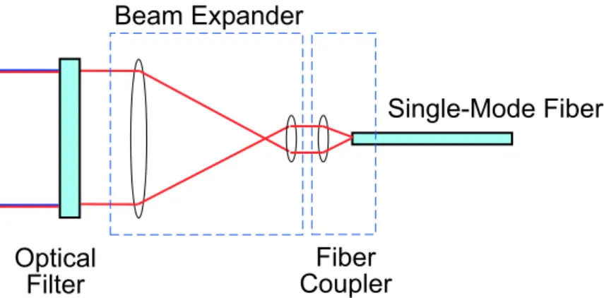
2-8 The optically-preamplified, direct-detection channel uses a telescope and objective lens to couple a single spatial mode into a single-mode fiber. Again, an optical filter passes the desired signal wavelengths while rejecting extraneous light sources at other wavelengths. . . 61

2-9 Heterodyne receivers mix the received optical field with a spatially and temporally coherent local oscillator, and extract the beat-frequency component in the resulting photocurrent. . . 62

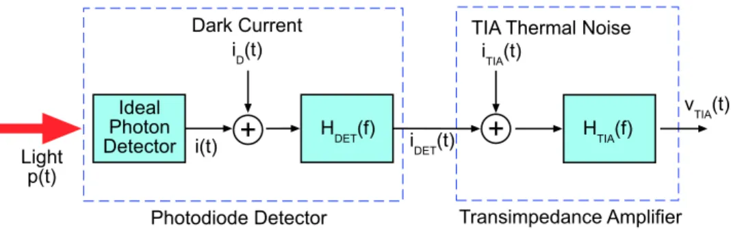
2-10 A common way to implement a direct-detection receiver is with a pho-todiode and a transimpedance amplifier. The phopho-todiode produces a current, which the transimpedance amplifier (TIA) converts to a mea-surable voltage. . . 66

2-11 This diagram illustrates the noises and bandwidth limitations of a prac-tical direct-detection receiver. . . 66

2-12 This block diagram shows an optical noise adding to the received opti-cal field f (t). For simplicity, we will assume the fields are normalized such that p(t) is the STA optical power. . . 68

2-13 Our second direct-detection channel employs intensity, or pulse ampli-tude modulation (PAM), modulation, atmospheric propagation, and optically-preamplified demodulation. . . 71

2-14 An optically preamplified receiver consists of an optical amplifier (e.g., an erbium-doped fiber amplifier (EDFA)), optical filter, photodiode detector, and transimpedance amplifier. . . 72

2-15 A coherent-detection receiver mixes a spatially- and temporally-coherent local oscillator with the incoming field. The STA power cross-term, which is proportional to the received field, then propagates through an ideal bandpass filter for subsequent processing. . . 75

(16)

3-1 The average capacity when both transmitter and receiver know the path gains is plotted versus the number of transmit and receive aper-tures (N = M ). We assume a unity receive noise power spectral density, i.e., N0 = 1, and that the Rayleigh fading does not on av-erage attenuate or amplify the transmitted power, i.e., var[<{αnm}] = var[={αnm}] = 1/2. We constrain the total transmit average power, E[x†_{x], to be no greater than P . . . .} ₈₂

3-2 The average capacity when only the receiver knows the path gains is plotted versus the number of transmit and receive apertures (N = M ). We assume a unity receive noise power spectral density, i.e., N0 = 1, and that the Rayleigh fading does not on average attenuate or amplify the transmitted power, i.e., var[<{αnm}] = var[={αnm}] = 1/2. We constrain the total transmit average power, E[x†_{x], to be no greater} than P . . . 84

3-3 The probability of pairwise codeword error, Pr( X → ¯X; ρ, η2_{), as a} function of the normalized fading strength η2 _{for total signal-to-noise} ratio ρ = M Ed/N0 = 8, 13, 15, and 18 dB. The limits as η2 approaches zero (3.42) are shown as circles. . . 96

3-4 The CLT probability of pairwise codeword error, Pr( X → ¯X; ρ, η2_), is plotted as a function of the normalized fading strength η2 _{for ρ =} M Ed/N0 = 18 dB. The smallest achievable error probability occurs when η2 ₌ e4σχ2₋₁

M N ≈ 3 × 10−2, or equivalently, when A = Ed

NI. . . 97 3-5 The smallest values of M and N such that (3.44) holds in mild fading

(σ2

χ = 0.01). In other words, orthogonal designs are optimal in the CLT regime for aperture numbers greater than these threshold values. 100

3-6 The smallest values of M and N such that (3.44) holds in moderate fading (σ2

χ= 0.1). . . 100 3-7 The smallest values of M and N such that (3.44) holds in severe fading

(σ2

(17)

3-8 A comparison of the pairwise error probability for A = Ed

NI STCs using the exact error probability in (3.48) computed via Monte Carlo averaging, the central limit theorem approximation (3.24) calculated via trapezoidal integration, its asymptotic behavior in (3.41), and the frustration function bounds in (3.50) and (3.52) computed via saddle-point integration. . . 103

3-9 The difference in SNR required to achieve a 10−6 _{pairwise codeword} er-ror probability between the actual lognormal erer-ror expression in (3.48) and its central limit theorem approximation in (3.24) is shown for dif-ferent fading strengths (σ2

χ= 0.01, 0.1, and 0.35). . . 105

3-10 The two transmit aperture (N = 2), BPSK, Alamouti STC, average codeword error probability is plotted for different numbers of receive apertures (M = 1, 2, and 4) and fading strengths (σ2

χ= 0.01, 0.1, and 0.35). Error bars indicate the standard error of each estimate. . . 108

NI STCs in moderate fading (σ2

χ = 0.1) using the exact error probability in (3.48) computed via Monte Carlo averaging, the central limit theorem approximation (3.24) calculated via trapezoidal integration, its asymp-totic behavior in (3.41), and the frustration function bounds in (3.50) and (3.52) computed via saddle-point integration. . . 111

N I STCs in weak fading (σ2

χ = 0.01) using the exact error probability in (3.48) computed via Monte Carlo averaging, the central limit theorem ap-proximation (3.24) calculated via trapezoidal integration, and the frus-tration function bounds in (3.50) and (3.52) computed via saddle-point integration. . . 112

(18)

4-1 With no average power constraint, the the parallel-channel upper bound (PC-UB) is the sum of concave functions evaluated at their respective maxima, whereas the the OOK lower bound (OOK-LB) is the maxi-mum of the their sum. In this two receive aperture (M = 2) example, C_PC−UB = h1(R1pmax1 ) + h2(R2pmax2 ), and COOK−LB = h1(R1pmax) + h2(R2pmax). . . 131

4-2 The maximum of hm(Rmp) as a function of sm lies between 1/e ≈ 0.3679 for low noise (sm → 0) and 1/2 for high noise (sm → ∞). . . . 132 4-3 In general, the upper and lower bounds on channel capacity are quite

close. This figure shows the fractional difference between the PC-UB and OOK-LB for the N = 2, M = 3 special case whose path gains are given in Table 1. . . 135

4-4 A photon-bucket receiver adds the photon counts from the M detectors to form a doubly-stochastic Poisson process. . . 136

4-5 Using an OOK transmitter and photon-bucket receiver with a threshold decision rule creates a binary-input, binary-output discrete memoryless channel. . . 136

4-6 This figure shows the maximizing duty cycle (4.73) as a function of noise-to-signal ratio s and interval length ∆. The solid red lines are the asymptotes (4.69) and (4.76). These two asymptotes coincide at 1/e as s → 0 and ∆ → 0. . . 146 4-7 This figure shows the capacity of the OOK transmitter and

unit-threshold receiver for different interval lengths ∆ and noise-to-signal ratios s. From top to bottom, the curves correspond to ∆ = 0, 0.1, 0.5, 1, 2, and 10 seconds. . . 147

(19)

4-8 The average capacity without average power constraint (σ = 1) for two (N = 2) identical transmitters (A1 = A2 = 1) and three (M = 3) receivers (λ = λ1 = λ2 = λ3) is shown as a function of background noise power λ. The parallel-channel upper bound (PC-UB) and OOK lower bound (OOK-LB) from [25] are shown along with the photon-bucket lower bound (PB-LB). All of these bounds have been averaged over 20,000 channel realizations of moderate fading intensity (σ2

χ = 0.1). The average capacity results for the high and low noise regimes, viz., (4.79), (4.83), and (4.86), are shown as lines, along with the capacity of a unit path gain channel (σ2

χ = 0) and its high noise asymptote (4.84).153 4-9 The probability that the channel can support a given rate is shown for

the low noise regime in moderate fading (σ2

χ = 0.1) with no average power constraint (σ = 1). The solid lines are the lognormal approx-imation of (4.110) and the symbols are the empirical complementary cumulative distribution of 300,000 channel capacity realizations. We assume that the identical transmitters (A1 = · · · = AN = 1) and receivers (λ = λ1 = · · · = λM) know and use the path gains optimally. 162 4-10 The rate achieved 99% of the time is plotted versus the number of

transmit and receive apertures in the low noise regime in moderate fading (σ2

χ= 0.1) with no average power constraint (σ = 1). . . 163 4-11 The probability that the channel can support a given rate is shown for

the high noise regime in moderate fading (σ2

χ = 0.1) with no average power constraint (σ = 1). The solid lines are the lognormal approxi-mation of (4.110) using the exact moments of the lognormal sum, see (4.102) and (4.104). The dashed lines are also the lognormal approxi-mation using approximate moments of the lognormal sum, see (4.106) and (4.108). The symbols are the empirical complementary cumula-tive distribution of 300,000 channel capacity realizations. We assume that the identical transmitters (A1 = · · · = AN = 1) and receivers (λ = λ1 = · · · = λM) know and use the path gains optimally. . . 164

(20)

4-12 The rate achieved 99% of the time is plotted versus the number of transmit and receive apertures in the high noise regime in moderate fading (σ2

χ= 0.1) with no average power constraint (σ = 1) . . . 165

4-13 The probability that the channel can support a given rate for ten trans-mit and ten receive apertures (N = M = 10) in the high noise regime for strong fading (σχ2 = 0.35) with no average power constraint (σ = 1). The solid line is the lognormal approximation of (4.110) using the exact moments of the lognormal sum, see (4.102) and (4.104). The dashed line is also the lognormal approximation using approximate moments of the lognormal sum, see (4.106) and (4.108). The symbols are the empirical complementary cumulative distribution of 300,000 channel capacity realizations. . . 166

4-14 The probability that the channel can support a given rate for one hun-dred transmit and one hunhun-dred receive apertures (N = M = 100) in the high noise regime for strong fading (σ2

χ = 0.35) with no average power constraint (σ = 1). The solid line is the lognormal approxi-mation of (4.110) using the exact moments of the lognormal sum, see (4.102) and (4.104). The dashed line is also the lognormal approxima-tion using approximate moments of the lognormal sum, see (4.106) and (4.108). The symbols are the empirical complementary cumulative dis-tribution of 3,000 channel capacity realizations (only 3,000 realizations were used due to limited computational resources). . . 167

5-1 The average capacity for OOK spatial repetition transmitters and equal-gain combining receivers using near-optimal thresholds is shown as a function of log-amplitude variance and average optical power per bit at each receiver, i.e., P = N A/2. The standard error (sample stan-dard deviation divided by the square root of the number of samples) on each estimate is less than 10−3_{. . . 193}

(21)

5-2 The average capacity for OOK spatial repetition transmitters and max-imal ratio combining receivers using near-optmax-imal thresholds is shown as a function of log-amplitude variance and average optical power per bit at each receiver, i.e., P = N A/2. The standard error on each estimate is less than 10−3_{. . . 195}

5-3 The bit error rate versus outage probability in the low noise regime using equal-gain combining and near-optimal thresholding is shown as a function of log-amplitude variance and aperture number. The solid lines depict the approximation (5.37), while the symbols are the em-pirical complementary cumulative distribution function of 100,000 bit error rate realizations. Note that the two transmitter, single receiver curve is not equal to the one transmitter, two receiver curve because we have defined P to be the average power per receiver. Consequently, the two transmitter system transmits half the power of the two receiver system. . . 201

5-4 The bit error rate versus outage probability in the high noise regime us-ing maximal ratio combinus-ing and near-optimal thresholdus-ing is shown as a function of log-amplitude variance and aperture number. The solid lines depict the approximation (5.37) using approximate moment matching, while the symbols are the empirical complementary cumu-lative distribution function of 100,000 bit error rate realizations. . . . 202

5-5 The average bit error rate for different transmitter and receiver diver-sity schemes with midpoint thresholding (5.12) is shown as a function of average power per receiver and number of apertures in mild fading (σ2

χ= 0.01). . . 206 5-6 The average bit error rate for different transmitter and receiver

diver-sity schemes with midpoint thresholding (5.12) is shown as a function of average power per receiver and number of apertures in moderate fading (σ2

(22)

5-7 The average bit error rate for different transmitter and receiver diver-sity schemes with midpoint thresholding (5.12) is shown as a function of average power per receiver and number of apertures in strong fading (σ2

diver-sity schemes with near-optimal thresholding (5.14) is shown as a func-tion of average power per receiver and number of apertures in mild fading (σ2

di-versity schemes with near-optimal thresholding (5.14) is shown as a function of average power per receiver and number of apertures in moderate fading (σ2

χ = 0.1). . . 210 5-10 The average bit error rate for different transmitter and receiver

diver-sity schemes with near-optimal thresholding (5.14) is shown as a func-tion of average power per receiver and number of apertures in strong fading (σ2

χ= 0.35). . . 211 5-11 A comparison of the exact and approximate average bit error rate for

equal gain combining receivers with near-optimal thresholding (5.14) is shown as a function of average power per receiver in mild fading (σ2

equal gain combining receivers with near-optimal thresholding (5.14) is shown as a function of average power per receiver in moderate fading (σ2

equal gain combining receivers with near-optimal thresholding (5.14) is shown as a function of average power per receiver in strong fading (σ2

χ = 0.35). In strong fading, our lognormal approximation provides a conservative estimate of error probability. . . 214

(23)

5-14 The average (over one million channel realizations) bit error rate for dif-ferent diversity techniques with midpoint thresholding (5.12) is shown as a function of average power per receiver in strong fading (σ2

χ = 0.35).217 5-15 The average (over one million channel realizations) bit error rate for

different diversity techniques with near-optimal thresholding (5.14) is shown as a function of average power per receiver in strong fading (σ2

χ= 0.35). . . 218

6-1 The experimental configuration for a single transmit and receive aper-ture system consists of an externally modulated laser transmitter and optically-preamplified, direct-detection receiver. Test equipment such as the BERT and DCA analyze the communication system perfor-mance, such as the eye diagram shown here. . . 222 6-2 This figure plots the measured and theoretical BERs versus the

av-erage received optical power for 1.25 Gbps data rates using midpoint thresholding (5.12) in the absence of fading (fiber transmission) for single and dual receiver configurations. . . 225 6-3 This figure plots the measured and theoretical BERs versus the average

received optical power for 1.25 Gbps data rates using midpoint thresh-olding (5.12) in mild fading (σ2

χ ≈ 0.02) for single and dual receiver configurations. . . 226 6-4 The empirical probability density function of the log-amplitude, i.e.,

0.5 log( Signal Power in mW ), for the first receiver is shown with its Gaussian fit. . . 227 6-5 The empirical probability density function of the log-amplitude, i.e.,

0.5 log( Signal Power in mW ), for the second receiver is shown with its Gaussian fit. . . 228

(24)

(25)

List of Tables

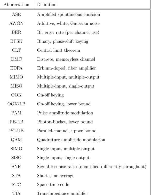
1.1 This table displays common symbols used throughout the thesis. . . . 42 1.2 This table displays common abbreviations used throughout the thesis. 43

3.1 Average capacity [nats/use] with path gain knowledge at the transmit-ter and receiver is shown as a function of aperture number (M = N ), fading strength (σ2

χ), and distribution (lognormal versus Rayleigh). The total transmit average power is constrained to be no greater than P = 10 dB. . . 81 3.2 Average capacity [nats/use] with path gain knowledge at the receiver

is shown as a function of aperture number (M = N ), fading strength (σ2

χ), and distribution (lognormal versus Rayleigh). The total transmit average power is constrained to be no greater than P = 10 dB. . . 85 3.3 Minimum distance pairwise error probability at Eb/N0 = 3 dB is

shown as a function of log-amplitude variance (σ2

χ = 0.1 and 0.01) for the Alamouti STC using two transmit and two receive apertures (N = M = 2). The columns are as follows: the exact pairwise error probability (LN) in (3.48), the central limit theorem (CLT) approxi-mation (3.24), and the frustration function bounds (Fr LB and Fr UB) in (3.50) and (3.52). . . 112 3.4 This table compares the Alamouti STC code error rate (Figure 3-10) at

Eb/N0 = 3 dB to the union bound estimates (twice the minimum dis-tance pairwise error probability) using the pairwise error probabilities in Table 3.3. . . 113

(26)

4.1 Path gains for the upper and lower bound comparison in Figure 4-3 . 134

4.2 This table shows bounds on the MIMO Poisson channel capacity for a given channel realization. The photon-bucket lower bound assumes a receiver structure that does not use path gain knowledge. The other two bounds assume the receiver knows and uses the path gains opti-mally. All three bounds assume that the transmitter optimally uses path gain knowledge. In the low and high signal-to-noise ratio (SNR) regimes, however, the transmit optimal duty cycles do not require path gain knowledge. In the high and low signal-to-noise ratio regimes, the optimal duty cycles converge, i.e., popt

m = popt = qopt, and equal min(1/e, σ) and min(1/2, σ), respectively. . . 141

5.1 This table shows the nominal parameters of the 1.25 Gbps testbed used in this chapter. These parameters represent a best case scenario with negligible background and thermal noise, ideal quantum efficiency, and minimum ASE noise. . . 191

5.2 Equal-gain combining average capacity [nats/use] from Figure 5-1 for an average optical power per bit at each receiver of P = −62 dBm. The standard error (sample standard deviation divided by the square root of the number of samples) on each estimate is less than 10−3_{. . . 194}

5.3 Maximal ratio combining average capacity [nats/use] from Figure 5-1 for an average optical power per bit at each receiver of P = −62 dBm. The standard error on each estimate is less than 10−3_{. . . 196}

5.4 The average total receive power (M P for combining schemes, and P for selection diversity) in dBm required for 10−5 _{average bit error rates} in severe fading (σ2

χ= 0.35) is shown for different diversity and thresh-olding schemes. The accuracy of the power is approximately ±0.1 dBm. The power gained in decibels from using a near-optimal versus a midpoint threshold is shown in the right most column. . . 219

(27)

6.1 This table summarizes the parameters of the OC-24 experimental testbed. The dark power, transimpedance amplifier thermal noise, and back-ground power were negligible compared to the amplified spontaneous emission noise; hence, these entries are marked not appreciable (n/a). 223

(28)

(29)

Chapter 1 Introduction

An estimated 95 percent of United States buildings are within 1.5 km of fiber-optic communication infrastructure, but currently unable to access it. One factor con-tributing to this inability is the high cost of optical fiber installation, approximately $100,000–$200,000 per kilometer in metropolitan areas, with trenching costs respon-sible for 85 percent of the total. Point-to-point optical communication through the atmosphere (i.e., wireless optical communication) has the potential to provide giga-bit per second data rates at roughly one-fifth the price of ground-based, fiber-optic technologies [65].

Communicating optically through the atmosphere, however, poses many inherent challenges. Bad weather (e.g., fog, snow, rain, etc.) and atmospheric molecular con-stituents (e.g., carbon dioxide and oxygen molecules) cause absorption and scattering that degrade the performance of optical communication systems. Furthermore, the temporal and spatial evolution of thermal inhomogeneities in the troposphere under clear weather conditions cause random fluctuations in the refractive index at opti-cal wavelengths [62]. These refractive-index perturbations—usually referred to as atmospheric turbulence—lead to amplitude and phase fluctuations on light beams propagating through the atmosphere [62], [31]. These fluctuations, in turn, have profound effects on the performance of laser communication systems operating over turbulent paths [49].

(30)

re-ceiver multiple copies of the transmitted message, each corrupted separately by the atmosphere. In this thesis, we will develop such methods to establish reliable com-munication through the turbulent atmospheric channel.

1.1 Optical Detection

We will examine two methods of converting an optical field into an electrical signal. Direct detection refers to receivers that respond only to optical power, i.e., the mag-nitude squared of the optical complex field. If the inherent randomness in photon arrivals is much greater than thermal noise, we can count the individual photons and make decisions based on photon arrival times. More realistically, we can use a condi-tional Gaussian approximation to examine the influence of all the noise sources that arise in a practical communication system.

In contrast to direct detection, coherent detection receivers mix the incoming optical field with a spatially and temporally coherent local oscillator. This heterodyne structure essentially yields a traditional additive, white Gaussian noise channel.

Our main focus will be exploring spatial and temporal diversity using multiple transmit and receive apertures. We will derive the information-theoretic capacity of communication, and study coding techniques for two direct detection and one coherent detection atmospheric channels. The first direct-detection channel uses ideal photon-counting receivers. The second direct-detection channel employs op-tical preamplification. The last channel uses coherent-detection receivers. Finally, we will experimentally verify, through hardware implementation, the benefit of receiver diversity using optically-preamplified, direct-detection receivers. Chapter 2 explains these channels in more detail.

1.2 Channel Capacity

Roughly speaking, channel capacity is the maximum rate of reliable communication [14, 21]. Although atmospheric losses are random, they are approximately constant

(31)

on intervals less than one to ten milliseconds [50]. Because typical data rates can exceed a billion bits per second, a block of several million bits can experience, on average, similar fading conditions.

This block fading model lends itself to many different information-theoretic no-tions of capacity [5, 44, 56]. Without any delay constraints, we can code over many channel realizations and achieve reliable communication rates up to the Shannon ca-pacity, defined as the average maximum mutual information per unit time, where the average is taken with respect to the random path gains [24]. Denoting the path gains of an N transmit, M receive aperture system as α = { αnm | 1 ≤ n ≤ N, 1 ≤ m ≤ M }, the ergodic capacity is the expectation with respect to the path gains of the instantaneous capacity, i.e., E[C(α)], [44, 66]. The ergodic assumption requires that communication occurs over several atmospheric coherence times, which allows coding across both “good” and “bad” channel realizations.

In practice, however, delay constraints may prevent coding over many channel realizations. In this case, the strict Shannon capacity is zero because there is a chance that the fading might be so egregious that the instantaneous capacity is below any desired rate [24, 5]. In this case, a more appropriate measure of capacity is the probability that the channel can support a desired rate. The capacity Cp per outage probability p is given by [5]

p = Pr {C(α) ≤ Cp} . (1.1)

In other words, the capacity per outage probability p is the p-th percentile of the instantaneous capacity, C(α), distribution. The channel can support data rates up to the outage capacity Cp with probability 1 − p.

We will examine the ergodic and outage capacities for our three atmospheric communication channel models. We are particularly interested in how the capacity scales with the number of transmit and receive apertures. These capacities will also depend on whether the transmitter and/or receiver know the path gains.

(32)

1.3 Space-Time Coding

Space-time codes (STC) refer to multiple transmitters sending codewords to multiple receivers over multiple time periods. For example, let xn(t) represent the symbol sent on the n-th transmit aperture during the t-th time period. A space-time codeword is then a matrix Tx 1 Tx 2 _{· · ·} Tx N t = 1 x1(1) x2(1) · · · xN(1) t = 2 x1(2) x2(2) · · · xN(2) ... ... ... . .. ... t = T x1(T ) x2(T ) · · · xN(T )

Tarokh in [61] established space-time code design criteria for Rayleigh and Ricean fading channels. These design criteria specify the pairwise properties of codewords from the space-time code. We will develop similar criteria for the coherent detection channel model, and demonstrate the reliability improvement gained through STCs.

For example, Figure 1-1 shows the pairwise error probability for a two transmit, one receive antenna, Alamouti STC in Rayleigh fading as a function of signal-to-noise ratio [1]. The Alamouti STC uses two transmit apertures and two time-slots to send two complex symbols s1 and s2 according to the schedule

Tx 1 Tx 2 t = 1 s1 s2 t = 2 _−s∗

2 s∗1

In Chapter 3, we will examine the performance of the Alamouti STC under lognormal fading for coherent detection receivers.

Tarokh demonstrated that the Alamouti STC is an example of a complex orthogo-nal design STC [60]. We will also show in Chapter 3 that orthogonal designs minimize the pairwise error probability for heterodyne systems using many apertures. Figure 1-2 shows that an orthogonal design space-time code can greatly reduce the effects of atmospheric turbulence on the error probability.

(33)

0 5 10 15 20 25 30 35 40 10−8 10−7 10−6 10−5 10−4 10−3 10−2 10−1 100 Rayleigh Fading Signal−to−Noise Ratio

Pairwise Error Probability

No STC

Alamouti STC

Figure 1-1: Space-time codes can improve the reliability of communication on fading channels. The shaded areas lie between upper and lower bounds on the pairwise error probability achieved in Rayleigh fading with and without an Alamouti space-time code. The bounds are plotted as a function of signal-to-noise ratio. In this case, the signal-to-noise ratio is the ratio of transmitted codeword energy difference to the receiver noise variance per real dimension.

(34)

−6 −4 −2 0 2 4 6 8 10 12 10−10 10−9 10−8 10−7 10−6 10−5 10−4 10−3 10−2 10−1 100

Lognormal Fading (

σ

_x2

=0.1)

(1/N)(E_d/N_o) [dB]

Pairwise Error Probability

MN=16 (Orthogonal Design STC) M=N=1 (No STC)

Figure 1-2: The pairwise error probability in moderate (σ2

χ = 0.1) lognormal fading is shown for an orthogonal design STC using coherent detection receivers. The product of transmit (N ) and receive (M ) aperture numbers is M N = 16. The error probability is plotted against the ratio of energy difference between codewords at the transmitter (Ed) per transmit aperture (N ) and receiver noise power spectral density (N0). Also shown is the single transmit, single receive aperture (M = N = 1) error probability when no space-time code is used.

(35)

1.4 Summary of Main Results

The main theoretical results of this thesis appear in Chapters 3 through 5, catego-rized by the type of receiver structure. Chapter 3 explores quadrature amplitude modulation and coherent detection receivers. Chapters 4 and 5 examine intensity modulation and direct detection reception. Experimental results appear in Chapter 6. We present background material necessary for understanding the channel models in Chapter 2.

Figure 1-3 shows multiple lasers and detectors providing spatial diversity to com-bat the effects of atmospheric fading. All the results of this thesis are based on this multiple-input, multiple-output (MIMO) channel model.

x1(t) y1(t) Laser Detector x2(t) y2(t) Laser Detector xN(t) yM(t) Laser Detector a11 aNM aN1

Figure 1-3: Providing the receiver with multiple copies of the transmitted message can improve the reliability of communication. This thesis explores the capacity of and coding for this multiple-input, multiple-output (MIMO) fading channel.

Roughly speaking, reliable communication occurs when not all of the paths in Figure 1-3 are deeply faded. This redundancy is an example of the old adage, “don’t put all your eggs in one basket.” We will demonstrate that “good” space-time codes for both coherent and direct detection cause the receiver to “see” the sum of path gain powers, i.e., the sum of squared magnitude complex field path gains.

Another theme of this thesis is to develop reliable communication systems that do not depend heavily on the tails of the fading distribution. Although we will argue in Chapter 2 that a lognormal distribution is an appropriate description of atmospheric

(36)

fading, experimental results indicate that atmospheric log-amplitude fluctuations are not Gaussian deep into the tails of its distribution [13]; for example, see Figures 6-4 and 6-5 in Chapter 6.

We will try to design communication systems that are insensitive to the tails of the fading distribution. In fact, many of our results only rely on the first and second moments of the fading distribution. Furthermore, several of our results are based on moment-matching approximations. By quantifying when these approximations are valid, we are essentially specifying the operating conditions in which the system design is insensitive to the distribution’s tails.

1.4.1 Coherent Detection Receivers

In Section 3.1, we use Monte Carlo averaging to calculate the average capacity of the coherent detection channel, assuming the transmitter and receiver know the path gains. We show that the ergodic capacity is not very sensitive to the fading strength or distribution. We compare this to the average capacity when only the receiver knows the path gains. As with Rayleigh fading channels [22], the benefit of knowing the path gains at the transmitter is negligible for moderate numbers of apertures and transmit power.

In Section 3.2, we present a space-time channel coding technique for overcom-ing turbulence-induced fadovercom-ing in an atmospheric optical heterodyne communication system that uses multiple transmit and receive apertures. In particular, a design criterion for minimizing the pairwise probability of codeword error in a space-time code is developed from a central limit theorem approximation. This design criterion maximizes the mean-to-standard-deviation ratio of the received energy difference be-tween codewords. It leads to STCs that are a subset of the previously reported STCs for Rayleigh channels, namely those created from orthogonal designs.

Our approach also extends to other fading channels with independent, zero-mean path gains. Consequently, for large numbers of transmit and receive antennas, STCs created from orthogonal designs minimize the pairwise codeword error probability for this larger class of fading channels. We published these space-time coding results in

(37)

[27].

1.4.2 Photon-Counting Receivers

In Section 4.1.1, we examine the Shannon capacity of the single-user, multiple-input, multiple-output Poisson channel with peak and average transmit power constraints. The MIMO Poisson channel is a good model for the physical layer of a multiple-aperture optical communication system that operates in the shot-noise-limited regime with known path gains. We derive upper and lower bounds on the capacity that coincide in a number of special cases. The capacity is bounded below by that of the MIMO channel with an additional on-off keying (OOK) transmitter constraint, and it is bounded above by that of parallel, independent, multiple-input, single-output (MISO) channels. We published these MIMO Poisson channel capacity results in [25].

We then consider the ergodic capacity and capacity-versus-outage probability of photon-counting, direct-detection optical communication through the turbulent atmo-sphere using multiple transmit and receive apertures. We assume shot-noise-limited operation in which detector outputs are doubly-stochastic Poisson processes whose rates are proportional to the sum of the transmitted powers, scaled by lognormal random fades, plus a background noise. With constraints on peak and average power per transmit aperture, we will show that at high signal-to-noise ratio, the ergodic capacity scales as the number of transmit apertures (N ) times the number of receive apertures (M ), and can be achieved with neither transmitter or receiver knowing the path gains. In the low signal-to-noise ratio regime, ergodic capacity scales as M N2_. In this regime, path-gain knowledge provides minimal capacity improvement when using a moderate number of transmit apertures. Furthermore, in the high and low signal-to-noise ratio regimes, we show that the ergodic capacity of this fading channel equals or exceeds that for a channel with deterministic path gains. In other words, we demonstrate that fading actually increases capacity.

We also develop expressions for the capacity-versus-outage probability in the high and low signal-to-noise ratio regimes by means of a moment-matching approximation

(38)

to the distribution of the sum of lognormal random variables. Monte Carlo sim-ulations show that these capacity-versus-outage approximations are quite accurate for moderate numbers of apertures in moderate fading. These ergodic and outage capacity results are submitted for publication [26].

In Section 4.2, we examine space-time coding for photon-counting receivers. We show that a switching space-time code can perform as well as the capacity-achieving repetition spatial code.

1.4.3 Optically-Preamplified Receivers

Theory

In Chapter 5 we examine the use of optical amplifiers to improve communication reliability. We develop lower bounds to the capacity of this channel by constructing discrete-memoryless channel representations. These representations utilize repetition on-off keying (OOK) spatial coding transmitters and linear combining, threshold-decision receivers. We show that equally weighting the detector outputs minimizes the error probability when the average receive power is much greater than -56 dBm (using the nominal parameters of the 1.25 Gbps testbed in Chapter 6). For lower average receive powers, weighting the detector outputs in proportion to their signal-to-noise ratio, i.e., classical maximal-ratio combining, is the best linear combining strategy.

Experiment

We also build a 1.25 Gbps testbed using optical preamplification. We demonstrate the benefits of using two receivers and equal-gain combining with midpoint thresholding. In mild fading, this configuration requires about three decibels less power per receiver to maintain a 10−6 _{bit error rate as compared to a single aperture system. We} also measure the distribution of the log-amplitude fluctuations on each receiver, and compare them to their theoretical Gaussian distributions.

(39)

1.4.4 Some Intuition: Paul Revere’s Dilemma

In this thesis, we will show that equal-gain combining is a capacity-achieving receiver architecture for the photon-counting channel at high signal-to-noise ratio. Similarly, equal-gain combining minimizes the bit error rate for optically-preamplified receivers at high signal-to-noise ratio. The following anecdote captures the intuition behind these results.

Digital, wireless, optical communication is a very old form of communication. In fact, the Sexton Robert Newman used it to notify Paul Revere that the British were coming. By the presence or absence of lamps in the Old North Church, Newman signalled optically one of three messages, or log₂_{(3) ≈ 1.6 bits of information: the} British are coming by land, they are coming by sea, or they are not coming at all.

Now suppose that Newman only cared about communicating whether or not the British were coming, but he was occasionally forgetful. If a lamp appears in the tower, then it is certain that the British are coming. But if no lamp appears, it means that either the British are not coming with probability 1 − p, or that they are coming with probability p, and he simply forgot to light a lamp. Under these circumstances, how does Paul Revere know when to ride? What rule should he use to minimize the probability of making the wrong decision: either riding in vain, or failing to respond to the British invasion?

The decision rule that minimizes the probability of error, is to choose the most probable scenario (British coming or not coming) given the observation (lamp present or not present). If Paul sees a lamp, then he should definitely ride because a lamp indicates that the British are definitely coming. If he does not see a lamp, then by taking no action, there is a probability p of failing to respond to an invasion. On the other hand, if he does ride, there is a probability 1 − p that he does so without need. So, if Newman only occasionally forgets, i.e., p < 1/2, then he should not ride if he does not see a lamp.

To further complicate matters, suppose that the weather is bad that night, and that visibility is poor. As a result, Paul might not see the lamp when glancing up at

(40)

the tower, even if it is there. Now, what should he do? An obvious solution would be to do more than just glance, but to stare up at the tower. If rain obscures the tower for one moment, it might not do so the next. Averaging temporally over the weather conditions reduces the uncertainty that not seeing a lamp is due to poor visibility. In wireless communication systems, this form of redundancy is sometimes called temporal diversity.

But what if Paul needed to know right now, at this moment, whether or not he should ride? He could position other riders so that they each had a different view of the tower, and they could all glance up at the same time. If anyone sees the lamp, then Paul knows for sure that the British are coming, and that he should ride. If each vantage point has a different visibility, then the chances that no one will see the lamp, if it is indeed there, is small. This form of diversity is known as receiver spatial diversity in wireless communication systems.

If the British are coming, then Newman could also place another lamp in a different tower, separated sufficiently in distance, so that the visibility of each tower is most likely different. This redundancy in wireless communications is called transmitter spatial diversity. In fact, it is an on-off keying (OOK) repetition spatial code.

If Paul or any other rider see either lamp, then they should ride. Equivalently, they could add up the number of riders that saw a lamp, and ride if this sum is greater than or equal to one. This strategy is equivalent to an equal-gain combining, threshold-decision receiver in wireless communications. In this case, equal-gain combining with unity threshold, minimizes the probability of making a wrong decision.

How does this anecdote relate to the results of this thesis? For photon-counting receivers operating at high signal-to-noise ratio, an absence of light impinging on the photodetector results in no photon counts with certainty. In other words, if all trans-mit lasers turn on and off simultaneously, and if any detector sees a photon during a bit interval, then we are certain that all transmitters were on, i.e., the British are coming. Indeed, in Chapter 4 we will show that OOK repetition spatial coding and equal-gain combining with unity threshold detection is a capacity-achieving commu-nication architecture for the atmospheric fading channel at high signal-to-noise ratio.

(41)

We observe a similar result for error probability in Chapter 5 for optically-preamplified receivers.

1.5 Notation and Abbreviations

Although we will try to remain consistent with notation throughout the thesis, we will redefine some notation between chapters for clarity. For example, we will always denote the path gain from transmitter n to receiver m as αnm. For coherent detection channels, this path gain is the complex field path gain, while it is the real power path gain (magnitude squared of field gain) for direct detection channels. Thus, in the background and coherent detection chapters (Chapters 2 and 3), αnm will denote the complex field path gain. For the direct detection chapters (Chapters 4 and 5), however, we will redefine αnm to be the power path gain, instead of using the cumbersome notation |αnm|2. We will similarly do so for the transmitted signal xn(t). Furthermore, the average number of photons per second is a more convenient measure of power for photon-counting receivers as it corresponds to the rate of the Poisson counting process. On the other hand, measuring power in Watts is more natural for optically-preamplified receivers because of the physical measurements recorded in Chapter 6. Tables 1.1 and 1.2 describe the major notation and abbreviations in this thesis.

(42)

Notation Definition

N Number of lasers

M Number of detectors

xn(t) n-th transmitter symbol/waveform at time t ym(t) m-th detector output at time t

αnm Path gain (field or power) from transmitter n to receiver m α _{Set of path gains {α}11, . . . , αN M}

χnm Atmospheric log-amplitude fluctuation φnm Atmospheric phase fluctuation

σ2

χ Atmospheric log-amplitude variance (fading strength) X, ¯X Transmitted codewords; channel input

Y Received signal; channel output

Q(x) Area under upper tail of standard normal density function

(43)

Abbreviation Definition

ASE Amplified spontaneous emission AWGN Additive, white, Gaussian noise BER Bit error rate (per channel use) BPSK Binary, phase-shift keying

CLT Central limit theorem

DMC Discrete, memoryless channel EDFA Erbium-doped, fiber amplifier MIMO Multiple-input, multiple-output

MISO Multiple-input, single-output

OOK On-off keying

OOK-LB On-off keying, lower bound PAM Pulse amplitude modulation PB-LB Photon-bucket, lower bound PC-UB Parallel-channel, upper bound

QAM Quadrature amplitude modulation SIMO Single-input, multiple-output

SISO Single-input, single-output

SNR Signal-to-noise ratio (quantified differently throughout)

STA Short-time average

STC Space-time code

TIA Transimpedance amplifier

(44)

(45)

Chapter 2 Background

In this chapter we will give a brief overview of optical communication through the atmosphere. For more complete references see [20] or [46].

2.1 Optical Communications

Conveying digital information via optical frequencies through the atmosphere is one of mankind’s oldest forms of communication. For example, fire beacons lit on mountain peaks relayed news of Troy’s fall in Aeschylus’s play Agamemnon, written in 5th century B.C. Also, early naval communication relied heavily on signalling flags and shuttered lamps ([23], pg. 1).

With the advent of the laser, however, came a new era in optical communication systems. Figure 2-1 shows a block diagram of a modern optical communication sys-tem. An information source generates bits that the coder uses to modulate the optical field of a laser carrier. The resulting field propagates through a medium such as a fiber optic cable, free space, or the atmosphere. The detector converts the optical signal to an electrical signal, and the decoder tries to infer the transmitted codeword. The term channel refers to the combined modulation, propagation, and demodu-lation processes that the transmitted codeword undergoes to reach the decoder. In this thesis, we will consider three atmospheric channels. All three channels will in-corporate propagation through the turbulent atmosphere. This propagation causes

(46)

Source Coder Laser Medium Detector Decoder Channel

Fiber Optic Cable Atmosphere

Figure 2-1: A modern optical communication system modulates a laser to convey information through a medium to a receiver. The receiver decodes the detected light and attempts to reconstruct the transmitted message.

fluctuations in the amplitude and phase of the received optical field. The extended Huygens-Fresnel principle models these fluctuations as a complex, lognormal random process [49].

The three channels we will study differ in their transmitter and receiver structures. Two channels use direct-detection (square-law or power) receivers, but vary in their models’ idealizations. The first direct-detection channel uses amplitude (intensity) modulation at the transmitter and ideal photon-counting detectors at the receivers. In this case, each detector output is a doubly-stochastic Poisson counting process whose rate is proportional to the short-time average (STA) optical power impinging on the detector.

The second direct-detection channel uses intensity modulation and optically-preamplified, direct-detection receivers. We will model this more realistic channel output as a

Gaussian process with a signal-dependent covariance. We will experimentally verify, through hardware implementation, the benefits of receiver diversity for this channel.

The final channel uses quadrature amplitude modulation (QAM) and heterodyne or coherent detection. Conditioned on the lognormal propagation fading, this channel behaves like an additive, white, Gaussian noise (AWGN) channel [20].

The next three subsections explain the modulation, demodulation, and propaga-tion models in more detail.

(47)

2.2 Atmospheric Optical Propagation

2.2.1 General Propagation Effects

Light travelling through the atmosphere experiences a number of degradations. Aerosols, molecules1_{, and thermal inhomogeneities in the atmosphere cause absorption and} scattering of the transmitted optical field. Absorption and scattering also cause at-tenuation of the transmitted field, resulting in an irretrievable loss of signal energy. Scattering gives rise to beam, angular, multipath, and Doppler spread. Beam and angular spread are illustrated in Figure 2-2. Beam spread is the apparent increase of divergence angle as the beam propagates from transmitter to receiver. Angular spread is the apparent broadening of the angle subtended by the transmitter as seen at the receiver. Angular spread is sometimes called the “shower curtain” effect, referring to the broadening of a light source when viewed through a shower curtain. Multipath spread is the lengthening of the transmitted pulse shape, which could possibly lead to intersymbol interference in digital communications. For line-of-sight propagation in clear weather, multipath spread is at most a few picoseconds and we will neglect it in all that follows [49]. Doppler spread manifests as time-dependent fading. The at-mospheric coherence time (reciprocal Doppler spread) is on the order of milliseconds, so that at gigabit per second data rates, the fading is flat over a great many symbols [49].

The refractive-index fluctuations induced by space- and time- varying thermal in-homogeneities are responsible for the twinkling of stars at night, and the shimmering above pavement on a hot summer day. As we shall see, these random amplitude fluctuations (called scintillation) can routinely be on the order of 10 dB, and last for several milliseconds. This receiver power outage leads to bursts of errors in wire-less optical communication systems [49]. This thesis primarily focuses on mitigating atmospheric fading using multiple transmit and receive apertures.

1_{Examples of aerosols relevant to optical propagation are water droplets, ice, dust, and organic}

materials of size comparable to the optical wavelength. Depending on the communication wave-length, molecular constituents that influence optical propagation include H2O, CO2, O3, O2, and

(48)

Detector Laser Beam Spread Angular Spread Atmospheric Turbulence h₁e jq1

...

h_ke jqk

...

h_Ke jqK

Figure 2-2: Light propagating through thin slabs of clear, turbulent atmosphere ex-perience random amplitude and phase fluctuations. The cumulative effect of these variations is approximately lognormal in distribution due to the central limit theorem. Scattering also causes spreading of the transmitted beam, and an apparent increase in the angular extent of the source at the receiver.

2.2.2 Atmospheric Propagation Models

We will confine our attention to optical communication in clear weather conditions for which absorption is negligible. As noted earlier, an optical signal propagating through the clear atmosphere experiences random amplitude and phase fluctuations as it passes through thermal pockets that vary on the order of 1o_{K. The refractive} index of clear air is temperature dependent. Consequently, as these thermal pockets mix and flow, they create eddies of refractive index turbulence. These eddies result in constructive and destructive interference of the propagating light.

The Thin-Screen Atmospheric Model

A simple, but useful, model of atmospheric propagation through turbulence is shown in Figure 2-2. This model divides the atmosphere into K thin slabs. Light propagating through each slab experiences a random amplitude and phase fluctuation, hkejθk.

(49)

Taken collectively, these variations result in the atmospheric path loss Y hkejθk = exp ³X log hk+ j X θk ´ −→ K→∞exp (χ + jφ) . (2.1)

The log-amplitude, χ =Plog hk, and phase, φ =Pθk, are sums of random variables and hence tend to a jointly Gaussian distribution via the central limit theorem. As a result, the light’s variation in amplitude and phase as it travels from transmitter to receiver is approximately lognormal in distribution.

We will generally assume that the atmospheric losses are random, but approxi-mately constant during each codeword transmission. Or alternatively, that the code-word length is small compared to the coherence time of the channel, yet large enough that information-theoretic notions such as capacity are meaningful. We justify this assumption by noting that the coherence time for the turbulent atmosphere is on the order of 1 to 10 ms [50], and typical data rates for line-of-sight communication in clear weather are on the order of a gigabit per second. Hence, 1 to 10 million con-secutive bits can experience on average similar fading conditions. This quasi-static fading model seems reasonable for our application.

We further assume that the turbulence-induced fading is frequency non-selective, i.e., there is a scalar multiplicative relationship between each transmitter and receiver path. The absence of multipath components at nanosecond durations in line-of-sight optical communication justifies this model [49].

Without loss of generality, we can separate the total atmospheric field attenuation, α, into two components, α = a0a. The non-random component a0 is due to the irretrievable power loss from absorption and scattering. The random component a = exp[χ + jφ] results from turbulence-induced fading.

The non-random component of atmospheric attenuation is described by

a0 = e− 1

2σZ, (2.2)

where Z is the propagation distance in kilometers. The power-attenuation coefficient σ consists of scattering and absorption components. Usually, aerosol and Mie

(50)

scatter-ing factors dominate this coefficient [45]. Assuming that aerosol absorption is small compared to the Mie scattering [38], we have that

σ ≈ 3.91_V µ λ 550 nm ¶−q(V ) , (2.3)

where λ is the optical wavelength in nanometers, V is the visibility in kilometers, and q(V ) is the size distribution of the scattering particles given by

q(V ) =          1.6 V > 50 km (High Visibility) 1.3 _{50 km ≥ V > 6 km (Average Visiblity)} 0.585V1/3 _{6 km > V} _{(Low Visibility)} . (2.4)

Figure 2-3 plots the atmospheric power-attenuation per kilometer in dB, i.e., −20 log10(a0)/Z, assuming that Mie scattering losses are the dominating factor at λ = 1550 nm. This figure illustrates that communicating in heavy fog can be ex-tremely difficult due the hundreds of dB/km in attenuation. For more information on communicating through optical scattering channels see [35],([34], pg. 211), or ([20], pg. 291). In this thesis, we will ignore absorption and scattering, and set a0 = 1.

Attenuation per km of Mie Scattering at 1550nm

0.01 0.1 1 10 100 1000 0.1 1 10 100 Visibility [km ] A tt e n u a ti o n p e r k m [ d B ] Thick Fog Moderate Fog Thin Fog Haze Light Haze Clear Snow Rain

Figure 2-3: Mie scattering can cause an irretrievable loss in optical power. This figure shows the atmospheric power-attenuation per kilometer at the 1550 nm wavelength for a variety of visibility and weather conditions. For example, in clear weather, the visibility is greater than 10 km, and attenuation is less than one decibel per kilometer.

(51)

The random variable a = exp[χ + jφ] represents the fading component of the atmospheric attenuation α. We will choose the mean mχ and variance σ2χ of χ such that the fading does not, on average, attenuate or amplify the optical power, i.e., E[|α|2_{] = a}2

0. Doing so requires

E£_|a|2¤= E£e2χ¤= Mχ(2) = 1, (2.5) where Mχ(s) is the moment-generating function of a Gaussian random variable given by Mχ(s) = exp µ mχs + 1 2σ 2 χs2 ¶ . (2.6) Hence, choosing mχ= −σχ2, (2.7)

makes the average power loss due to atmospheric fading unity [50].

We can further simplify matters by assuming that the phase of the received op-tical field is uniformly distributed over [0,2π), and is independent of the amplitude fluctuations. This assumption is equivalent to making φ statistically independent of χ, with zero mean and a very large variance, i.e., var[φ] À 2π.

The Extended Huygens-Fresnel Principle

The extended Huygens-Fresnel principle [49] models the diffractive nature of light, and provides the basis for a more thorough treatment of propagation through the turbulent atmosphere. Because the polarization-dependent effects of the atmospheric turbulence are negligible, we can assume that the electric field of the propagating optical signal is linearly polarized, i.e., it is a scalar function of space and time. We will represent this scalar field at a three-dimensional location r ∈ R3_{, where R is the} set of real numbers, and at a time t using the complex quasi-monochromatic notation

(52)

where u(r, t) is a complex-valued scalar function whose temporal bandwidth is much less than the carrier frequency, fc, and <{x} denotes the real component of x. We also assume that the complex field u(r, t) is normalized such that h|u(r, t)|2_{i is the} short-time average (STA) power of the optical field per unit area, i.e.,

STA Power per Unit Area ≡ h|u(r, t)|2i ≡ 1 TSTA

Z t t−TSTA

|u(r, τ)|2dτ, (2.9) where h|u(r, t)|2_{i has units Watts per meters squared. The integration period T}

STA > 0 is much greater than the reciprocal of the optical carrier frequency and any radio frequency (RF) sub-carrier frequency differences, but much less than the reciprocal of the information-bearing bandwidth of the signal. This integration period will be made more precise later when we consider the bandwidth limitations of practical detectors.

Example:

Suppose u(r, t) is the scalar optical field of a wavelength-division multi-plexed signal with information bearing sub-carrier frequencies f1, f2 ¿ fc, i.e.,

u(r, t) = u1(r, t)e−j2πf1t+ u2(r, t)e−j2πf2t, (2.10)

where u1(r, t) and u2(r, t) have temporal bandwidths much less than their sub-carrier frequencies. The STA power of the optical field is

h|u(r, t)|2i = 1 TSTA Z t t−TSTA ¯ ¯u1(r, τ )e−j2πf1τ + u2(r, t)e−j2πf2τ ¯ ¯2 dτ = 1 TSTA Z t t−TSTA ¡ |u1(r, τ )|2+ |u2(r, τ )|2 +2<©u1(r, τ )u∗2(r, τ )e−j2π(f 1−f2)τª¢ dτ ≈ |u1(r, t)|2+ |u2(r, t)|2,

where x∗ _{denotes the complex conjugate of x, and 1/T}

STAis much greater than the temporal bandwidths of u1(r, t) and u2(r, t), but much less than the frequency difference between sub-carriers, f1− f2.

(53)

Figure 2-4 provides a reference frame for our multi-aperture communication sys-tem consisting of N transmit and M receive pupils. The n-th transmit pupil is located at σn ∈ R2 in the z = 0 plane. It produces a field that propagates in the +z direction. Using the coordinates σ ∈ R2 _{in the z = 0 plane, denote this field as}

sn(σ, t) =    u ([σ, 0], t) = pn(σ)xn(t), σ ∈ {n-th Tx Pupil} 0, otherwise , (2.11)

where we have assumed that the modulator at each transmitter changes the tem-poral characteristics of the optical field (amplitude and phase), but not its spatial characteristics. We can then separate the the spatial pn(σ) and temporal xn(t) field components over the n-th transmit aperture.

The total field in the z = 0 plane is the sum of the fields over each transmit aperture, s(σ, t) = u ([σ, 0], t) = N X n=1 sn(σ, t) = N X n=1 pn(σ)xn(t). (2.12)

The extended Huygens-Fresnel principle relates the complex field in the z = 0 plane to the complex field in the z = Z plane. Denote the field in the receiver plane as

r(ρ, t) = u([ρ, Z], t), (2.13)

where ρ ∈ R2 _{are the spatial coordinates in the z = Z plane. Under the} parax-ial assumption that the propagation distance is much greater than the receiver and transmitter pupil diameters, then the field in the receiver (z = Z) plane is

r(ρ, t) = Z

s(σ, t − Z/c) hFS(ρ − σ) eχ(σ,ρ)+jφ(σ,ρ)dσ, (2.14) where c is the speed of light, { χ(σ, ρ), φ(σ, ρ) } are jointly Gaussian random processes with known mean and covariance functions, and hFS(ρ) is the paraxial free-space Green’s function, hFS(ρ) = 1 jλZe jk³Z+kρk_2Z2´ , (2.15)

(54)

1y

1x

1z

z=0

z=Z

n-th

Transmitter

Pupil

m-th

Receiver

Pupil

Z meters

Atmosphere

s

₁

r

_M

r

₁

s

₂

s

_N

D

_TX

_D

RX

d

_TX

d

_RX

Figure 2-4: The geometry for the extended Huygens-Fresnel principle consists of the n-th transmitter pupil located at σn in the z = 0 plane and the m-th receiver pupil located at ρm in the z = Z plane. In this diagram, 1x, 1y, and 1z are unit vectors marking the origin.

Capacity of and Coding for Multiple-Aperture, Wireless, Optical Communications

Capacity of and Coding for Multiple-Aperture,

Wireless, Optical Communications

by

Shane M. Haas

B.S. Mathematics, University of Kansas (1998)

B.S. Electrical Engineering, University of Kansas (1998)

M.S. Electrical Engineering, University of Kansas (1999)

M.A. Mathematics, University of Kansas (1999)

Submitted to the Department of Electrical Engineering and Computer

Science

in partial fulfillment of the requirements for the degree of

Doctor of Philosophy in Electrical Engineering

at the

MASSACHUSETTS INSTITUTE OF TECHNOLOGY

May 2003

c

° Massachusetts Institute of Technology 2003. All rights reserved.

Author . . . .

Department of Electrical Engineering and Computer Science

May 14, 2003

Certified by . . . .

Jeffrey H. Shapiro

Julius A. Stratton Professor of Electrical Engineering

Thesis Supervisor

Accepted by . . . .

Arthur C. Smith

Chairman, Department Committee on Graduate Students

Capacity of and Coding for Multiple-Aperture, Wireless,

Optical Communications

by

Shane M. Haas

Abstract

Acknowledgments

Contents

List of Figures

List of Tables

Chapter 1

Introduction

1.1

Optical Detection

1.2

Channel Capacity

1.3

Space-Time Coding

No STC

Alamouti STC

Lognormal Fading (

σ

=0.1)

1.4

Summary of Main Results

1.4.1

Coherent Detection Receivers

1.4.2

Photon-Counting Receivers

1.4.3

Optically-Preamplified Receivers

1.4.4

Some Intuition: Paul Revere’s Dilemma

1.5

Notation and Abbreviations

Chapter 2

Background

2.1

Optical Communications

2.2

Atmospheric Optical Propagation

2.2.1

General Propagation Effects

...

...

2.2.2

Atmospheric Propagation Models

1y

1x

1z

z=0

z=Z

n-th

_D