HAL Id: hal-01719925
https://hal.archives-ouvertes.fr/hal-01719925v3
Submitted on 29 Oct 2018
HAL is a multi-disciplinary open access
archive for the deposit and dissemination of sci-entific research documents, whether they are pub-lished or not. The documents may come from teaching and research institutions in France or abroad, or from public or private research centers.
L’archive ouverte pluridisciplinaire HAL, est destinée au dépôt et à la diffusion de documents scientifiques de niveau recherche, publiés ou non, émanant des établissements d’enseignement et de recherche français ou étrangers, des laboratoires publics ou privés.
A Physical Vulnerability to Climate Change Index:
Which are the most vulnerable developing countries?
Mathilde Closset, Sosso Feindouno, Patrick Guillaumont, Catherine Simonet
To cite this version:
Mathilde Closset, Sosso Feindouno, Patrick Guillaumont, Catherine Simonet. A Physical Vulnera-bility to Climate Change Index: Which are the most vulnerable developing countries?. 2017. �hal-01719925v3�
fondation pour les études et recherches sur le développement international
LA FERDI EST UNE FOND
A TION REC ONNUE D ’UTILITÉ PUBLIQUE. ELLE ME T EN ŒUVRE A VEC L ’IDDRI L ’INITIA TIVE POUR LE DÉ VEL OPPEMENT E T
LA GOUVERNANCE MONDIALE (IDGM).
ELLE C
OORDONNE LE LABEX IDGM+ QUI L
’ASSOCIE A U CERDI E T À L ’IDDRI. CE T TE PUBLICA TION A BÉNÉFICIÉ D ’UNE AIDE DE L ’É T A T FRANCAIS GÉRÉE P AR L ’ANR A U
TITRE DU PROGRAMME «INVESTISSEMENT
S D
’A
VENIR»
POR
T
ANT LA RÉFÉRENCE «ANR-10-LABX
-14-01».
Revised version October 2018
A Physical Vulnerability to
Climate Change Index:
Which are the most vulnerable
developing countries?
Mathilde Closset | Sosso Feindouno
Patrick Guillaumont | Catherine Simonet
mathilde Closset is an associate economic aff airs offi cer at UNECLAC. Sosso Feindouno is a research assistant at FERDI.
Patrick Guillaumont is the president of FERDI. Catherine Simonet is a research fellow at ODI.
1. Introduction
The recognition of climate change as a dominant issue for the global economy and policy
has led to a search for resources for fi nancing mitigation and adaptation. While raising
funds for mitigation and for adaptation meet similar problems, their allocation between
countries cannot be ruled by the same criteria. For the concessional funds devoted to
adaptation allocation criteria should specifi cally refl ect the adaptation needs of the
recipient countries (beside their level of income and their capacity to eff ectively use
the funds). An appropriate indicator of vulnerability to climate change is then required
for guiding the allocation of adaptation resources. Not any indicator of vulnerability to
climate change can fi
t
this
purpose.
… /…
Acknowledgements
The authors want to particularly thank David Wheeler, and H.M. Fussel for their helpful comments on a previous version of this paper, as
De
velo
pment Ind
ica
to
rs
Wo
rkin
g Paper
213
December 2017…/… The 2015 year agenda was exceptional with the adoption of the new Sustainable Development Goals, for the fight against climate change (COP 21 Summit in Paris) and for risk disaster management (negociations on the post-Hyogo framework agreement). In the preparation of these events, the risk, vulnerability and resilience concepts have frequently been recalled1, as well
as the complexity of their design and assessment. For instance the International Panel on Climate Change (IPCC) report of the working group II (2014) has defined vulnerability index as “a metric characterizing the vulnerability of a system. A climate vulnerability index is typically derived by combining, with or without weighting, several indicators assumed to represent vulnerability”. Behind this broad definition encompassing all aspects of vulnerability, there does not seem to be an agreement on how these notions should be incorporated in the framework of the Sustainable Development Goals.
The search of an appropriate indicator of vulnerability to climate change can draw lessons from the past experience of development economics and policy. A relevant experience is that of the least developing countries (LDCs), designed as the poor countries facing most severe structural handicaps to development, and thus threatened to be locked into a poverty trap. A main structural handicap retained for their identification is a high structural economic vulnerability, captured in an index called Economic Vulnerability Index (EVI) (United Nations, 2015). This index is now considered not only as a criterion for the identification of the LDCs, but also as a relevant criterion for the allocation of development assistance (see UN Genaral Assembly resolution on the smooth transition of graduating LDCs –A/C.2/67/L.5– and a survey in Guillaumont, 2015).
Here, with the aim of combining the allocation of resources for poverty reduction and for adaptation to climate change in a consistent mannner, we propose an index of physical vulnerability to climate change built on principles similar to those of the UN Economic Vulnerability Index. As the EVI captures a “structural” economic vulnerability and supposed to be exogenous, the index of vulnerability to climate change should capture a “physical” vulnerabilty to climate change and thus exogenous. Such a vulnerabilty to climate change, independent of the present political will of the countries, is expected to identify countries needing the most adaptation assistance, regardless of their political choices, and is likely to be used as a criterion for the allocation of adaptation ressources. This index could then be combined with other indicators to determine an optimal allocation of these resources (Guillaumont,2015b).
The assessment of the vulnerability to climate change that is proposed is thus focused on the vulnerability which depends only on physical factors, factors which do not depend on the present will or policies of the countries, and are essentially geo-physical. This “Physical Vulnerability to Climate Change Index” (PVCCI) should offer a quantitative and comparative assessment of the vulnerability of developing countries in a synthetic way. It relies on a few components, both relevant and reliable, which are available for the whole set of developing countries, and which are easily
understandable, so that the index can be used in a transparent manner. Once calculated, this index of physical vulnerability to climate change shows a high degree of heterogeneity among countries, even within the same regional area or continent.
The remainder of this paper is organized as follows: Section2 presents the key features of an index of physical vulnerability to climate change likely to be used for operational purposes and differing from other various concepts of vulnerability in climate change research. Sections 3 provides a description of the components of the PVCCI. Next, the specific methodology used to build the PVCCI is presented in Section 4 and, the results for developing countries, not forgetting the robustness analysis. Section 5 concludes the paper with potential policy implications.
2. Required features of the new index of vulnerability to climate change
Beginning with the main definitions of vulnerability to climate change, this section tries to define physical vulnerability to climate change. The “vulnerability of systems to climate change” is examined in what has been a rapidly growing literature, relying on various fields of research, such as climate science, disaster management and development economics. It illustrates the “necessary greater synergy between ecologists and economics”(Wam, 2009).
2.1. General economic vulnerability versus structural economic vulnerability
The word ‘vulnerability’ has been used with various meanings and by many researchers in food security, natural hazards, disaster risk, public health, global environment, climate change or development economics (for a sample of applications of the concept of vulnerability in these various fields, see: Timmerman, 1981; Blaikie, 1994; Cutter et al., 1996; Guillaumont and Chauvet, 2001; McCarthy, 2001; UNEP, 2002 chapitre 3; Prowse 2003; Turner et al., 2003; Miola et al., 2015). In development economics, the notion of vulnerability has been used mainly at the microeconomic level (see for instance Dercon et al., 2005; Yamano et al.,2005). It has also been used at the macroeconomic level, with the search for measurable and comparable indices (this literature is reviewed in Guillaumont ,2009a, b).
In the macroeconomic context, the vulnerability of a country is taken as “the risk of being harmed by exogenous, generally unforeseen, events or shocks” (Guillaumont 2009a). Based on several decades of research (in particular on export instability), this macro vulnerability is now widely considered to be an impediment to growth. Economic vulnerability can be seen to consist of three main components: shock, exposure and resilience. Shocks are exogenous and generally unforeseen events (external e.g. the instability of exports, or natural, e.g. typhoons, hurricanes, earthquakes, droughts,…). Exposure corresponds to factors on which the direct impact of shocks depends. Resilience is the capacity to react to shocks. A weak resilience is, a part of the general vulnerability (Miller et al., 2010).
are considered, a general or overall vulnerability is assessed. When only the size of the exogenous shocks and the extent of exposure to these shocks are the only components considered, the vulnerability considered is essentially a “structural” vulnerability. Resilience, even if it may include some structural elements, is often related to policy factors. Structural economic vulnerability is the kind of vulnerability captured by the Economic Vulnerability Index (EVI), used by the United Nations to identify the Least Developing Countries (LDCs). This index intends to reflect the likely size of recurrent external or natural shocks, and the main structural factors of the exposure to these shocks, using a small number of indicators in a transparent manner . It refers mainly to vulnerability in low-income and lower middle low-income countries (see UN-CDP web-site and Guillaumont 2007, 2009a, 2009b).
The level of income per capita is indeed a major factor of economic resilience, but since this level is taken into account separately both officially for the identification of the LDCs and most often for the allocation of Official Development Assistance (ODA), it is not usually included in the measurement of structural economic vulnerability.
2.2. Structural or physical vulnerability to climate change: can it be identified?
Vulnerability to climate change is a vulnerability to environmental shocks resulting from climate change. These shocks are here considered as the physical expression of climate change. They essentially appear through the increase in the number and intensity of droughts, floods, and storms, as well as through the rise in sea level for low-lying coastal areas level regions; they are reflected by the change in the mean values of climatic variables (such as temperature or rainfall), and by related changes in the instability of these variables.
There has been a rich recent literature on vulnerability to environmental change and more specifically to climate change, as well as, partly overlaping, on vulnerability to natural hazards. Not surprisingly, there is no universally accepted definition of vulnerability to climate change.
The definition of vulnerability depends on its expected use and influences the orientation of the vulnerability analysis (O’Brien et al., 2007)2. First, the notions have been used with various meanings,
depending on the scientific field (Hinkel, 2008; Brückner, 2010). Second, within each field, various conceptual frameworks have been defined and no vulnerability assessment is superior to anotherThe choice of method depends on the objectives and the availability of data (kelly and Adger, 2000; de Sherbinin, 2014). As a result, the corresponding literature has been qualified as a “Tower of Babel” (Janssen and Ostrom, 2006). Facing this “tower” authors have suggested building a formalized common framework (Ionescu et al., 2009; Hinkel, 2008, 2011). Above mentioned authors agree that the multiplication of frameworks and definitions leads to blurring the message drawn
2 The main references to environmental vulnerability include Adger (1999), Kelly and Adger (2000), Olmos (2001), O’Brien et al. (2004), Downing and Patwardhan (2005), Yamano et al. 2005, Füssel (2007), Ionescu et al. (2009); and to vulnerability
from the analyses.
To identify the structural or physical vulnerability to climate change, it is useful to refer to the three usual components of economic vulnerability (size of the shocks, exposure to the shocks, resilience), and to consider that structural vulnerability is mainly captured through the shock and exposure components, while resilience is more related to policy or to other variables likely to be considered separately as the level of income per capita. Let us now briefly review the literature on vulnerability to climate change with the aim of seeing whether it isolates these structural or physical components of vulnerability to climate change. For the sake of this review, we identify three main approaches in the literature on vulnerability.
2.3. Main current approaches to climate change vulnerability
Let us call chronological approach (ex post versus ex ante) the sequential analysis of a shock climate change) that compares the situation before and after a shock. Kelly and Adger (2000) adopt this approach by defining an end point vulnerability and a starting point vulnerability. They define the “starting point vulnerability” as the body of elements in the environment that make ex ante the consequences of shocks worse.This vulnerability is affected by social and economic dynamics, and by political and institutional characteristics. The “end point vulnerability” results from the consequences of climate change. It is captured by an assessment of the losses from the shock, related to its characteristics and size. O’Brien et al. (2007) uses a similar distinction. The authors deal with an outcome vulnerability and contextual vulnerability whose definitions are close to the end point and starting point vulnerability of Kelly and Adger (2000). A similar distinction is also made in the Glossary of the last IPCC’s Working Group II report (2014), grouping the outcome vulnerability and end-point vulnerability on one hand and contextual vulnerability and starting-point vulnerability on the other hand.
What can be called an oignon approach consists of elaborating a progressively encompassing concept of vulnerability. The aim of this framework is to make the definition of vulnerability gradually more complex following different scales (often geographic scales). This type of analysis is proposed by Bogardi and Birkmann (2004) and developed in Birkmann (2007). The author considers the core of the vulnerability as intrinsic vulnerability. He introduces a continuum of definitions of vulnerability spanning from the tightest to the widest definition: “multi dimensional vulnerability encompassing physical, social, economic, environmental and institutional features” (Birkmann 2006).
The social and ecological dichotomic approach is a framework which finds its roots in the ecological literature. Adger et al. (2004) distinguish a biophysical vulnerability from the social vulnerability. This distinction is close to that presented by Brooks (2003) who identifies two kinds of vulnerability to climate change in the literature. Biophysical vulnerability is defined by environmental scientists in terms of physical damage caused to a system by a particular climate-related event or hazard (Nicholls
et al. 1999, Jones and Boer 2005); vulnerability being analyzed in terms of the likelihood of
occurrence and impact of weather and climate related events (Nicholls et al. 1999). The biophisical approach corresponds most closely to sensitivity in the IPCC concept and terminology; it is also associated with the risk assessment and risk management (Alwang et al., 2001).The second type of
vulnerability is defined as the “state that exists within a system before it encounters a hazard event” (Allen 2003). In this sense, it is close to the “starting point vulnerability” of Kelly and
Adger (2000). This is also, according to Brooks, the definition of social vulnerability. Social
vulnerability depends not only on biophysical factors, but also on the set of socio-economic factors that determine peoples’ ability to cope with stress or change (Allen 2003). It can be seen as including what has been called exposure and resilience factors, which involve both structural and policy factors. Cutter and Finch (2008) define social vulnerability as a measure of both the sensitivity of a population to natural hazards and its ability to respond to and recover from the impacts of hazards. The United Nations Development Program (2000) defines it as “… the degree to which societies or socioeconomic groups are affected by stresses and hazards, whether brought about by external forces or intrinsic factors (internal and external) that negatively impact the social cohesion of a country” (UNDP, 2000).The distinction made by Brooks (2003) led him to aggregate social and biophysical vulnerability into a unique system3.
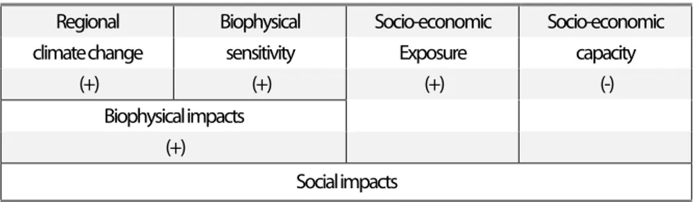
Finally, most influencial is the IPCC’s approach. The IPPC WGII report (2007) defines vulnerability as “the degree to which a system is susceptible to, and unable to cope with, adverse effects of climate change,” (IPCC 2007a, Glossary). This definition is close to the definition of economic vulnerability previously presented with the three overlapping components: shock, exposure and resilience. In Figure 1, the diagram given by Füssel (2010), helps to understand what in the IPCC definition concerns structural vulnerability and what does not: here “social impacts” should be understood as “vulnerability to climate change”.
Figure 1. Vulnerability to climate change framework, the reading of IPPC definition by Füssel (2010)
Regional Biophysical Socio-economic Socio-economic
climate change sensitivity Exposure capacity
(+) (+) (+) (-)
Biophysical impacts
(+)
Social impacts
This approach is reformulaled by the Special Report on Managing the Risks of Extreme (IPCC 2012) presenting a risk management approach and by the IPCC WGII Report ( IPCC, 2014a). The vulnerability is defined as “The propensity or predisposition to be adversely affected. Vulnerability encompasses a variety of concepts including sensitivity or susceptibility to harm and lack of capacity to cope and adapt”. The framework of the IPCC Working group II (IPCC, 2014a) is summarized in the Figure A2 (in Appendix). Vulnerability concept encompasses a part of the risk, hazards and exposure concepts and includes also sensitivity or susceptibility to harm, lack of capacity to cope and adapt components.
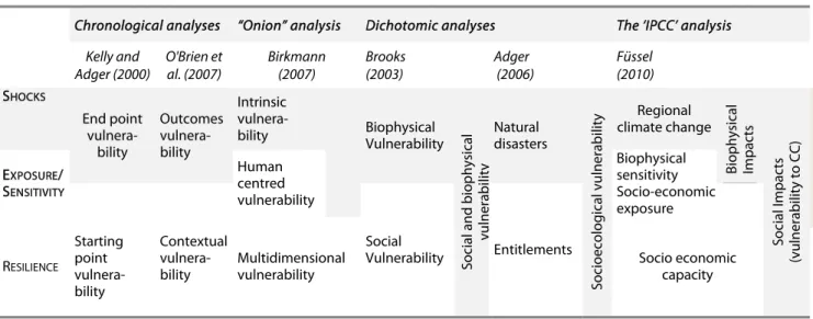
In the Figure 2, we show how all these approaches of vulnerability can be highlighted through a
simple decomposition: Shocks, exposure and resilience. When referring to environmental vulnerability to climate change, the distinction established with reference to macroeconomic vulnerability between shock, exposure and resilience should be kept in mind.
Figure 2. Vulnerability frameworks in the light of the shocks, exposure and resilience definitions
Chronological analyses “Onion” analysis Dichotomic analyses The ‘IPCC’ analysis
Kelly and Adger (2000) O'Brien et al. (2007) Birkmann (2007) Brooks (2003) Adger (2006) Füssel (2010) SHOCKS End point vulnera-bility Outcomes vulnera-bility Intrinsic vulnera-bility Biophysical Vulnerability Social a n d biop hysical vulnerabi lit y Natural disasters Socioec o logic a l vu lnerabi lit y Regional climate change Biophysi cal Impacts Social Impacts (vul nerabil ity to CC) EXPOSURE/ SENSITIVITY Human centred vulnerability Biophysical sensitivity Starting point vulnera-bility Contextual vulnera-bility Social Vulnerability Entitlements Socio-economic exposure RESILIENCE Multidimensional vulnerability Socio economic capacity
Note : Continuum of vulnerability concepts : In grey approximate delimitation the structural components of vulnerability.
This paper proposes a vulnerability assessment limited to the physical vulnerability. Relying on the experience of the LDCs identification and ODA allocation criteria permits to propose a “miror” indicator of the Economic Vulnerability Index (EVI), harmonizing in this way the two biggest issues of the next decades: poverty reduction and climate change. The permanent research of co-benefits called by international institutions (OECD, 2009) needs an harmonized and coherent approach in the allocation of funds for development and adaptation.
2.4. From analysis to measurement of vulnerability to climate change
The impact of climate change is not homogeneous within a country. Some effects will impact only a certain area in a given country, while others will have the same impact in the neighboring countries of a particular region. Although the choice of a national scale for the index does not correspond to homogeneous climate change characteristics, it can be used at the national level for the construction of the index from more disaggregated data. As noted at the beginning of the paper, the proposed index should be likely to be used as a criterion for the allocation of adaptation resources between countries, leading to allocate more resources to countries which are on average more vulnerable to climate change. For this reason, the choice of scale for the analysis is the country.
Another issue to be addressed is the heterogeneity of the source of vulnerability among countries. What matters for a country is not the simple average of the various sources of vulnerability, but its vulnerability to the source likely to have the highest impact in its case. For this reason, as we’ll see later, the indicator of the vulnerability to climate change resulting from various sources of vulnerability should be designed so that it can reflect a high vulnerability resulting from a specific factor.
The time frame of the index also raises an important issue. To what extent can the indicators rely on past trends and characteristics to assess vulnerability to future shocks? Components can be calculated as forecasts, i.e. on a purely ex-ante basis or ex-post, from the observation of current trends. It seems possible to rely on forecasts only when data are available and reliable (e.g. likelihood of sea level rises). Other components should be calculated ex-post from past trends and levels.
3. Components of the Physical Vulnerability to Climate Change Index (PVCCI)
The IPCC WGII report defines the climate change as “a change in the state of the climate that can be
identified (e.g., by using statistical tests) by changes in the mean and/or the variability of its properties, and that persists for an extended period, typically decades or longer”. This definition calls for a
distinction between two kinds of consequences and related risks: the risks of progressive shocks and the risks of increasing recurrent shocks. These two categories of risk roughly correspond to the first and the second categories of hazard identified by Adger et al. (2004).
Starting from the distinction between the risk of progressive shocks and the risk of an increase of the recurrent shocks, we try to identify reliable indicators that are good candidates to compose an index of physical vulnerability to climate change. Since it is unavoidably debatable to assess the final economic and social impact of climate change, indicators should rely on measurable intermediary consequences, estimated either directly or by the means of proxies. Thus, differing from other attempts to assess vulnerability to climate change, our assessment only considers the expected impact of climate change on physical variables. These variables are of course likely to have socio-economic consequences, but they are not socio-socio-economic variables. Using physical indicators means using only objective or neutral data. It avoids reference to indicators partly influenced by policy or resilience factors.
In any case, the set of indicators presented below should be considered as tentative. They try to capture the main channels through which climate change is a factor of vulnerability. It should be remembered that a good index should use a limited number of components, transparent and focused on the most relevant issues. The aim of the paper is to give a first flavour on what would represent this physical vulnerability, focussing only on physical dimension of vulnrability to climate change.
3.1. Risk of progressive and durable shocks
The risk of progressive shocks (or continuous hazard) refers to possible persistent consequences of climate change at the country level. The two main types of such risks, as identified in the literature, are rise of the sea level, which may lead to flooding, and increasing aridity, which may lead to desertification.
Risk of flooding from the rise of sea level: shock and exposure
The vulnerability of a country to the rise of the sea level is essentially the risk of this country being flooded. Its assessment involves making a distinction between the size of the shock (magnitude of the rise of the sea level) and the exposure to this shock (altitude). An assessment of the vulnerability of zones likely to be flooded then depends on the two following factors:
the exposure to sea-level rise depends on the relief, since it influences the likelihood of
flooding, so that the indicator should take into account the distribution of the heights of arable lands or the distribution of the population according to the height of occupied lands;
the shock could be estimated by the distribution of the likelihood of a sea-level rise in t future years.
The combination of the exposure and potential shocks allows for the assessment of the likelihood of flooding resulting from the sea level rise (in t years).
The measurement of the exposure component does not raise insuperable difficulties. Its assessment relies on a good knowledge of the geographical configuration of countries. If the index refers to the distribution of land heights, a possible matter of debate is the kind of area to be considered. If the distribution of the height of population location is referred to, a debate might arise about the expected change in this distribution over time : however since the future change may itself depend on the adaptation policy, there is a rationale in considering only the present distribution. Indeed the present structural vulnerability should not really depend on this change.
It is more difficult to assess the risk of the sea level rise, for two reasons. First, there is still some degree of uncertainty about the rise of the sea level on a given time horizon. Secondly, the probability distribution is changing over time with rising average sea levels and increasing dispersion. Let us suppose that we know the probability distribution of the sea level rise for each of the next t years. The impact on the expected percentage of flooded areas is consequently changing. This impact can be considered at a given future time (for instance +30 years or +50years, …) or all over agiven number of years. In this case should it be expressed as a present value, using a discount rate? This might be done for two reasons. The uncertainty of estimations is increasing as the time horizon is extending, although this growing uncertainty can be already captured by the increasing dispersion of the probability of the sea level rise. When the each year sea level rise is expressed only as an average level, then it would be legitimate to discount for this reason alone. A second reason would be the “pure time preference”: the disadvantage generated by a given sea level can be considered higher the earlier it occurs; the later it occurs, the higher the capacity of a country to face it. So a logical indicator would be the present value of the likelihood of flooded areas over the next t years.
1
(1)
With: SLR: sea level rise indicator;
i, country indicator and j, the meters of sea level rise;
hij, probability that the sea level rises by j meters for the i country;
and sij the part of arable lands below j meters in country i (or the share of population
living below j meters in country i); t: number of years from now; r: discount rate.
The discount rate can be the same for all countries. Indeed, as far as it reflects a pure time preference, it could differ across countries, but differences cannot be reliably assessed and they would then reflect differences in the capacity to adapt, a component of vulnerability which is not really “structural” and cannot clearly be considered for the allocation of adaptation resources.
Anyway one can consider arbitrary to apply any discount rate. Then, taking r =0, a simplified indicator could be the likely part of flooded areas in x years (the time horizon of x years being also arbitrary):
(2)
Risk of increasing aridity: assessment from past trends in temperature and rainfall, and from initial conditions
The literature on the consequences of climate change shows the risk of some arid countries (in particular Sahelian countries) being threatened by over-aridity (see for instance IPCC, 2014b). The risk depends both on the present level of temperature and rainfall (exposure) and on their trends (shock).
Proxies for the exposure to the risk of an increasing aridity can be either the actual average level of rainfall in the country, or preferably the actual part of dry lands in the country, which better fits the risk of desertification. The lower the rainfall level or the higher the dry lands percentage in a country, the more exposed the country to a long term decrease of rainfall or increase in temperature. As for the size of the shocks, it seems relevant to use the past trend (appropriately estimated) in annual average temperature over the past two or three decades, supposing it will go on. A similar and complementary proxy of the shock measurement for the risk of increasing aridity can also be found in a decreasing trend of the average rainfall level. At the country level, the progressive shock resulting from climate change, and evidenced in a rising trend in temperature or a decreasing trend
in rainfall, is thus captured by exploiting past trends. 3.2. Risk of increasing recurrent shocks
Climate change is also likely to generate more frequent or more acute natural shocks, such as droughts, floods, and typhoons (IPCC, 2014a). Here again the only variables to be considered should be unambiguously linked to climate and its change, such as the rainfall and temperature increasing variability, and the frequency of typhoons as well.
The vulnerability to increasing recurrent rainfall and temperature shocks has two main kinds of components, corresponding to the previous distinction between exposure and shocks. The exposure components are here given by the average frequency of past (rainfall, or temperature, or storms) shocks, which reflects the local climate, but not its change: this average frequency during previous years can be taken as a proxy to the exposure. The shock components, more forward-looking, are drawn from the trend in the frequency and intensity of the shocks, assuming this trend is determined by climate change, likely to go on in the future. These two kinds of components are considered in the same way for rainfall, temperature, and storms.
Average present frequency as an indicator of exposure
When the Economic Vulnerability Index (EVI) was developed at the United Nations by the Committee for Development Policy (CDP) for the identification of the Least Developed Countries, the risks of natural shocks were assessed ex-post by a measure of shock incidence over past years. Among the components of the EVI, indirect and synthetic indicators were used likely to capture highly heterogeneous natural shocks (floods, typhoons, droughts, hurricanes, and earthquakes) with highly unequal intensity and consequences.. The two related indicators of the EVI were an index of the instability of agricultural production (IA), and initially an index of the percentage of homeless
population due to natural disasters4 (HL), replaced since the review of 2012 by an indicator of the
percentage of population killed or affected by natural disasters.
The instability of agriculture production was a square deviation of the agricultural production with regard to its trend. These two indicators were averaged in a natural shocks index: NSI= (IA+HL)/2. Within the EVI, this natural shock index, although calculated ex-post, is considered as reflecting a risk for the future, due to the recurrent nature of the related shocks: the average past level is taken as a proxy for the risk of future shocks. This index is indeed likely to change over time, but a high past level can simultaneously be considered as generating a handicap to future economic growth. As for the vulnerability to climate change, the present approach is different. First, the average level of past shocks is related to rainfall and temperature, two variables clearly linked to climate, while the instability of agriculture production or homelessness (or the percentage of population killed or affected by natural disasters) also depends on shocks which are not all related to climate. Thus, the
4 The latter index comes from the Center of Research on Epidemiological Diseases which also produces other indicators,
index of exposure to climate change, relying on past average levels of rainfall or temperature instabilities, is unambiguously physical, and by no way influenced by policy or resilience factors. To measure instabilities, two methods can be applied. A simple way consists to use the absolute deviance of climate variables (rainfall or temperature) from their long-term trend. But, this method does not have good mathematical properties and is not widely used. Our preferred measurement is the instability calculated as square root of square deviation of climate variables from their long-term trend. For instance, the index of rainfall instability should be:
t t tR
R
R
IR
2)
ˆ
(
(3)with the trend level of .
Second, the past average level of shocks is considered as an indicator of the exposure to an increase
in the frequency and size of these shocks, which is captured by a specific index of the size of the shocks,
as explained below.
Trends in the intensity of past shocks as a proxy of future shocks
The risk of increasing recurrent shocks associated with climate change is here assessed in a look back manner. We assume that the more significantly the shock intensity has been increasing in the past, the more likely is a shock increase in the future. In other words, if rainfall and temperature shocks have increased due to climate change, they are assumed to remain increasing in the future. The proxy used will then be the trend in the size of instability.
For instance, the proxy for the risk of increasing rainfall shocks will be the (positive) trend in the squared (or absolute) deviation of the yearly average of rainfall from its own trend. For instance, supposing a linear trend, the indicator may be measured from:
t
R
R
R
t t tˆ
)
.
(
2 (4)with α being the trend in the intensity of rainfall instability. Assuming a non-linear trend, the measurement may be:
2 2 1 2.
.
)
ˆ
(
t
t
R
R
R
t t t (5)The index of the size of future (rainfall) shocks then will depend on the time horizon selected, as is the case for the rise of the sea level, as well as on the shape of the trend.
In the same way, it is possible to estimate an index of the size of future (temperature) shocks from the trend in the intensity of temperature instability (α’).
significant shocks, or typhoons as well, by designing significant shocks from given thresholds in the level of “bad events”, what could seem more arbitrary, but may appear more dicriminatory. We come back to this option when calculating the index.
Figure 3. Composition of the Physical Vulnerability to Climate Change Index
Note: The boxes corresponding to the two last rows of the graph respectively refer to exposure components (grayed-out, in italics) and to size of the shocks components.
In the above presentation, the physical vulnerability to climate change index gathers ten sub-components into five sub-components reflecting two kinds of shocks (progressive ones and increasing recurrent ones), following a unified framework.
4. Construction of the index
The physical vulnerability to climate change index has been calculated using data from 1950 to 2016, coveringsixty seven years. The index can be updated and calculated regularly.
4.1. Measurement of components: Data and methodology
Risk of flooding
It has not been possible to calculate the risk of flooding due to sea level rise according to the formula previously proposed because of a lack of agreed data on the evolution of the average level rise, and even more on the probability distribution of this rise. However,data allowed us to calculate the exposure to sea level rise, supposing a rise up to 1 meter.So, a convenient proxy for the risk of flooding due to sea level rise has been the index of the “relative part of country affected by a rise of 1 meter of the sea level”5. Furthermore, we investigate the robustness of this indicator by assessing
the impact of choosing an elevation threshold of 2 meters. It appeared that a possible choice of the elevation treshold of 2 meters instead of the one of 1 meter would not change results significantly. The Spearman’s rank correlation between the two measures is strongly significant and stands at 99.2%.
Countries with low elevation coastal zones are obviously the most exposed to the risk of flooding due to sea level rise. Nevertheless, it should not be forgotten that some of the most devastating floodings occur when glacial lakes overflow, in particular when the so-called Glacial Lake Outburst Floods (GLOFs) take place. The spectacular retreat of mountain glaciers is one of the most reliable evidence of climate change. Glaciers floods represent the highest and most far-reaching glacial risk with high potential of disaster and damages (Richard and Gay, 2003). For instance, in Bhutan, according to the International Centre for Integrated Mountain Development (ICIMOD) annual report 2002, glaciers have been retreating and thinning at an average rate of 30-40 meters per year since the mid-1970s. A similar situation is observed in Nepal. A large part of these two countries are covered by the Himalaya Mountains which concentrate the bulk of outbursts from moraine-dammed lakes.These type of country need a specific treatment in the measurement of the risk of flooding due to climate change. Otherwise Bhutan and Nepal which are landlocked would be given a minimum score of 0, thus appearing non vulnerable because of their lack of access to the open sea. So in order to take into account of the serious risk of ice melting to which they are exposed, but which cannot be presently measured, their initial zero score has been replaced by the value standing at the top quartile of the the full sample.
5 Our elevation database was computed based on two digital terrain models (Shuttle Radar Topography Mission and
Share of dryland areas
Database on the exposure of drylands are based on the definition of dryland of the United Nations
Environment Program6. Our indicator is the part of dryland areas, considered to be the arid,
semi-arid, and dry sub-humid zones(three of the world’s six aridity zones), as a percent of the country’s (non desertic) total land area. For consistency’s sake, we exclude deserts (which are classified as hyper-arid areas) in both the dryland area and the country’s total land area. We used CRU TS 4.01
database to calculate the ratio7 of average annual precipitation to potential evapotranspiration
(P/PET), from which the definition of areas according to the degree of aridity is drawn.
Rainfall and temperature; levels,trends and instabilities
Rainfall and temperature data come from the Climate Research Unit (CRU TS version 4.01 – University of East Anglia), currently one of the most frequently used dataset, particularly by recent works on climate change. This version of database covers from 1901 to 2016. Monthly time series of temperature or rainfall are globally gridded to 0.5 x 0.5 degree spatial resolution on land areas8.
To calculate the trend of temperature and rainfall, we use the OLS approach, respecting fundamental principles of the OLS that there should not be autocorrelation between observations. The estimated coefficients obtained by the OLS from the monthly climatic data (especially monthly temperature data) might indeed be erroneous, since monthly temperature data violate the hypothesis of no dependance between observations: monthly data of temperature are not independent, hot months tending to follow hot months and cold months to follow cold months. This autocorrelation increasing the uncertainty in the trend may lead to spurious estimates of the trends.
To deal with this issue and assuming a linear9 trend, we apply a simple and consistent approach as
follows10:
for each country and per month of year, we regress the temperature (or rainfall) on the time
variable covering the 1950-2016 period using the following equations:
j
ij t
Temp
(6)Where Tempijis monthly temperature of country i in the month j since 1950;
6 UNEP definition of Arid, semi_arid and sub humid areas: Areas, other than the polar and subpolar regions, in which the
ratio of annual precipitation to potential evapotranspiration falls within the range from 0.05 to 0.65.
7 This ratio makes it possible to highlight the “degree of aridity” of a territory. Hyper-aridity (desert) is observed when the
ratio P/PET is less than 5 percent.
8 For countries where kriging points are not exactly in the country (13 countries), we use buffering technique and couple
the point closest to the country in the country where data are missing.
9 For simplicity, we assume a linear trend. One can check the validity of this assumption. For instance, in the previous version
of the PVCCI, a squared trend was also added in checking the robustness.
10 One can reduce the number of data points of the series, focusing on the number of independent observations. The final
effective sample size is determined by Neff N(1r1)/(1r1), where N is the original sample size,
r
1the lag-1 autocorrelation coefficient. The main harmful aspect of this technique is that it is burdensome and consumer of data.t
time variable and error term. for each country, we recover the twelwe estimated coefficients
(one by month); finally, the trend indicator is measured by the arithmetic mean of estimated coefficients by
country.
The same approach is implemented to monthly rainfall data even if these are less subject to the autocorrelation of observations.
The level of temperature and the level of rainfall is determined by the annual average of each of the two variables over the period 1950-2016, respectively.
Trends in shocks are determined by the regression of the residuals (in absolute value) obtained from the equation (8) on the time variable. In the benchmark PVCCI, we only take into account the negative shocks for rainfall and only the positive shocks for temperature. These trends in the absolute values of the negative rainfall shocks and in the positive temperature shocks are supposed to be related to climate change, with a potential impact all the more significant that the country is more arid.
Storm intensity
The literature on climate change seems to agree that storms are likely to become more intense. Differing from a previous version of PVCCI, this version includes a storm intensity component. Data
on storm duration and categories11 are obtained from the National Oceanic and Atmospheric
Administration – National Climatic Data Center – International Best Track Archive for Climate Stewardship (IBTrACS), version v03r06. From the perimeter of land area provided by this database, we compute the territory’s land area affected by the storms using the ArcGIS software. We use data from 1970 to 201412, period for which storms events are exhaustively recorded.
If a country is affected by several storms events during the same year, we add them. Thus, the storm intensity in a country i for the year t is computed as follows:
∑ ∑ ∝ (7)
Where
j
is a given storm event (total equal to n) observed in the countryi at theperiode
t
,k
the category of storm (6 categories ranking from 0 to 5), D theduration by storms categories (in hours) of the event
j
,S
the share of territory affected by storm category (expressed as a percentage of the total country area).
11 These categories correspond to Saffir-Simpson scale rating from 1 to 5. We also add the category of “other storms” to
which we assign the rate equal to 0.
12 Our last access on the site of the National Oceanic and Atmospheric Administration (September 2018) did not allow us
to obtain data on storms events beyond 2014. But with the recent events, we observe that the countries having very high scores before 2014 are those that have mostly been affected by recent storms events.
For each country, we compute the arithmetic mean of the storms intensity for each year over the 1970-2014 period, then the change in storms intensity. Storms being random phenomena with some countries experiencing them more than others, it may be difficult to highlight a consistent linear trend for each country. For this reason, we divide data into two periods. The first time period examined runs from 1970 to 1992 and the second from 1993 to 2014. The average storms intensity of each period has been computed for each country. The difference of the average storms intensity between the second period and the first period could be considered as a proxy of the trend in storms intensity.
4.2. Averaging the components
Each component is first normalized following the max-min method13:
∗ 100 (8)
With
CN : normalized component C: value of component
Aggregation:choosing a quadratic rather than arithmetic average
Each of the previous component indicators gives information which can be used independently from each other. Making available the measurement for each component and sub-component will allow researchers to use them separately or to combine them in an aggregated index. Indeed a synthetic index is also required, in particular, as underlined above, for aid allocation. The aggregation of the components, once they have been expressed as indices on a common scale, raises several issues.
The structure of the index can be presented in two ways. The first one, illustrated by Figure 3, distinguishes between risks related to progressive shocks and risks related to more intense recurrent shocks, both considered as resulting from climate change. The risks related to progressive shocks cover those due to (i) the sea level rise and (ii) the trends in average rainfall and temperature. The intensification of recurrent shocks corresponds to the increasing intensity of (iii) rainfall shocks, (iv) temperature shocks and (v) storms. The shocks are thus grouped into five components, each of them including both an exposure index (in italics) and a shock index has been computed. Another way of presenting the structure of the index, still starting from the distinction between risks related to progressive and recurrent shocks, is to split up the later into two mains sub-components: (a) the past average level of rainfall instability, temperature instability and storm intensity, a proxy for exposure, and (b) the trend in the instability of rainfall and temperature and the change in storms intensity, a proxy for the shock itself.
The way by which the values of the components are averaged is also an important issue. The usual averaging practice for the calculation of synthetic indices is the arithmetic one (as it is done for the Human Development Index or for the EVI). However, any of the main components of a vulnerability index may be of crucial importance for a country, more or less independently from the level of the other components. In that case, it is relevant to use an averaging method reflecting a limited substitutability between components (as already examined for the EVI in Guillaumont, 2009a). It can be obtained either by a reverse geometric average14 (as done in Ibid.), or, what is finally retained here,
a quadratic average of the components, defined in the following way:
n kA
n
G
1 21
'
(9)with Ak the index value of the k component.
The choice of the quadratic mean instead of the arithmetic mean is based on the concept that the vulnerability of a country may critically depend on the levels of only one or two components, whatever the level of the others. While all components bring some information about the vulnerability of a country, their variance should also be considered as an additional factor of vulnerability to climate change. The quadratic mean gives greater weight to larger values (and is equal to or greater than the arithmetic mean15). As an example, an island with a very large share of
area likely to be flooded and an arid country suffering from a highly increasing trend in the instability of the level of temperatures are both highly vulnerable, but each of these two countries, due to a specific component close to one, may be considered as highly vulnerable even if it is not vulnerable with respect to other components of the index. Thus a high vulnerability to climate change will be better evidenced by using the quadratic average, rather by an arithmetic average. A quadratic average evidences the vulnerability of each country in its specificity. The quadratic mean is used at two levels:
for the calculation of the PVCCI by averaging the five components of shocks;
although it may seem less necessary, for the calculation of each component, by the quadratic
average of the indices of the exposure to the shock and the size of the shock.
Weighting the components
A traditional aggregation issue is related to the weight given to each component. Since the components are forward-looking, it is not possible to determine the weights from an econometric estimation of the expected respective impact of each component on a global indicator of
14 Here, we prefer the quadratic average. Since each component varies from 0 to 100 because of normalization, the
multiplicative nature of the geometric average would reduce to zero the vulnerability of any country having a value of zero for at least one component irrespective of the values of the country in the others components.
15 It depends on the variance of the components according to the relationship:
development. Even for the structural economic vulnerability the respective impact of the EVI’s components on economic growth appeared quite difficult to apply (Guillaumont, 2009a). A simple and usual, although arbitrary, solution is to use equal weights. We propose here to attribute equal weigths (1/5) to the five components. A higher implicit weight is nevertheless given to the highest vulnerabilty component through the use of a quadratic average.
Other simple weightings are conceivable. Since the five components fall into two categories of risk (risks related to progressive shocks and risks related to more intense recurrent shocks), it may be valuable to attribute equal weight to the two kinds of risk. In other words, this amounts to assign weights of 1/4, 1/4, 1/6, 1/6 and 1/6 respectively to flooding due to the sea level rise or ice melting, increasing aridity, and to the intensification of rainfall shocks, temperature shocks and storms. Or since rainfall and temperature are two important climatic factors affecting agricultural production, especially in the context of climate change, it may be legitimate to aggregate the intensification of rainfall shocks and temperature shocks considering the interdependance between the two variables, although rainfall seems more important than temperature for crop yield. One could then assign weights of 1/4, 1/4, 1/8, 1/8, 1/4 respectively to flooding due to the sea level rise or ice melting, increasing aridiy, rainfall, temperature and storms.
These different choices of weighting could be applied considering all shocks of temperature and rainfall (symmetrical shocks) or just positive shocks of temperature and negative shocks of rainfall (asymmetrical shocks). Several options are possible and we do not report all of them. But they are available from the authors upon request.
4.3. Results
The PVCCI is calculated for a complete set of 191 (developed and developing) countries16. The
normalized scores are between 0 (the least vulnerable) and 100 (the most vulnerable). However, no country has a score equal to 0 or 100. The benchmark PVCCI exhibits a minimum value of 39.8 and the maximum value of 69.7, bringing a statistical range of 29.9. This would mean that all countries are facing climate change somehow, being vulnerable with respect to one or other components of the PVCCI. The index serves as a tool for determining to what extent the countries are physically vulnerable to climate change, and by which way they are so. Let us recall that the results presented below only concerns physical vulnerability: other important factors of the social vulnerability, in particular the level of income per capita and human capital, are not considered since they should be taken into account separately in the allocation of concessional resources for adaptation, as they are with respect to EVI in the identification of the LDCs.
According to the benchmark PVCCI, the “physically” most vulnerable countries to climate change are Oman (69.7), Marshall Islands (68.8), the Maldives (66.5)and the least vulnerable are Georgia (39.8), Nauru (39.9), New Zealand (40.3).The average score for the entire sample of the PVCCI stands at 52.8
16 We include both the developed and developing countries for two reasons. First, all countries are affected by climate
change, and it makes sense to provide a comprehensive view of the risks they face. Second, all countries may well be candidates for assistance in the uncertain.
while the median score stands at 51.8, showing that the scores in a few countries are clearly higher than the main part of the sample. The standard deviation indicates the heterogeneity across countries.
In what follows, we group countries under seven categories of particular interest for researchers and policy makers. Table 1 shows that SIDS and African countries are especially very vulnerable to climate change. Already structurally handicapped in their national development process, LDCs are also penalized by the climate change. PVCCI’s scores of LDCs presented in the Appendix A1 show that of the 15 most vulnerable countries in LDCs group, 12 are in Africa (all in sub-Saharan Africa). If we look at LDCs and moving from the most vulnerable to the least vulnerable, Sudan is ranked first. With the exception of Kiribati and Tuvalu, Sudan, Mauritania, Niger, Chad and Eritrea are at the same time the most vulnerable in LDCs group and African countries group. This is not surprising when we consider the components used in the PVCCI. Agriculture is one of the key vulnerable sectors identified by IPCC (2007b). But agricultural production in (sub-Saharan) Africa is severely compromised owing to the increasing temperatures, the increasing of arid and semi-arid land, the decreasing trend of rainfall. Most of African countries are among the most vulnerable in at least three of the five components. This, combined with the quadratic mean used in the aggregation procedure, increase the likelihood of finding African countries among the highest scores of the PVCCI.
The PVCCI’s average score of Small Island Developing States is also very high17. Given their inherent
physical characteristics (small size of country, low elevated coastal zone), SIDS are very prone to natural disasters: floods, earthquakes, tropical and extratropical cyclones, tsunamis, and so on. In many SIDS, the majority of human communities and infrastructure are located in coastal zones. They are the most vulnerable countries into the components of storms intensity and flooding due to sea level rise or melting glaciers.
The standard deviation values highlight a high heterogeneity across all country groups.. The PVCCI is relatively highly variable within the group of SIDS Non-LDCs and the vulnerability is likely to be greatest where local environments are already under stress as a result of human activities.
Table 1. Physical Vulnerability to Climate Change Index (PVCCI) by country groups
Country groups Mean Median Standard
Deviation Min Max Developing countries (144) 54.7 54.0 6.7 39.8 69.7 LDCs (48) 55.3 52.8 6.5 41.4 65.9 Non LDCs (96) 54.3 54.5 6.8 39.8 69.7 SIDS (36) 56.1 56.4 6.9 39.9 68.8 SIDS LDCs (9) 56.9 57.0 6.1 46.9 65.1 SIDS Non-LDCs (27) 55.9 56.3 8.4 39.9 68.8 African countries (54) 56.1 56.4.4 6.9 39.9 68.8
17 In the previous version of the PVCCI, the average score of SIDS was lower than the one obtained in the present version.
Note: The sample of developing countries (except Dominica) is the same as that used by the United Nations’ Committee for Development Policy (UN-CDP) since the 2015 triennial review for the Economic Vulnerability Index (EVI), Human Assets Index (HAI) and GNI per capita. We considered the 48 LDCs of the UN-CDP's 2015 triennial review.
4.3. Robustness and sensitivity analysis
The PVCCI hitherto built is based upon some methodological choices and assumptions, calling
for assessing the robustness of the index. Among a wide range of possible configurations, we
retain two relevant configurations18 used to test the robustness of the benchmark PVCCI. We
call them: PVCCI2 and PVCCI3. For ease of analysis, let us rename the five components of the PVCCI introduced earlier in Figure 3.Cluster 1 replaces henceforth “Flooding due to sea level rise or melting glaciers”
Cluster 2 replaces henceforth “ Increasing aridity”
Cluster 3 replaces henceforth “Rainfall”
Cluster 4 replaces henceforth “Temperature”
Cluster 5 replaces henceforth “Storms”
PVCCI 2
The aim here is to evaluate the impact of using an alternative way to calculate the instabilities. Instead of taking the squared deviation, the PVCCI2 uses the simple absolute deviation (of temperature and rainfall from their long-term trend). The rest remains unchanged: we still consider the quadratic mean and maintain the choice of negative shocks of rainfall and positive shocks of temperature.
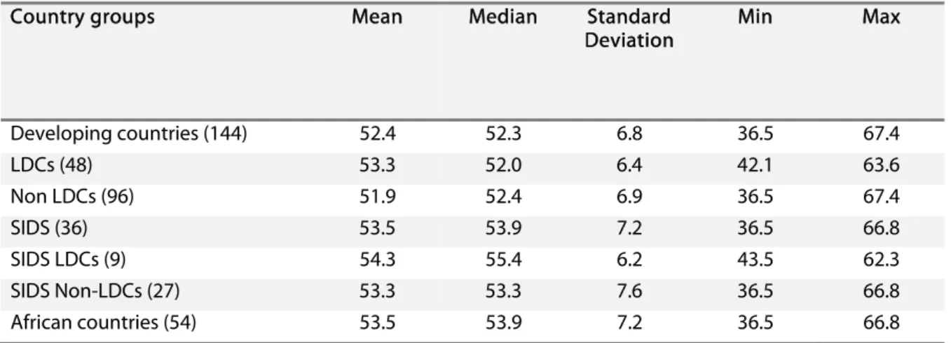
The scores of the PVCCI 2 for the whole sample range from 36.5 to 67.3, with an average of 50.5, a median of 49.1 and a standard deviation of 7.2. The three most vulnerable countries are identical to those of the benchmark PVCCI: Oman (67.3), Marshall Islands (66.8), the Maldives (65.0); the least vulnerable countries are Nauru (36.5) Georgia (37.8) , New Zealand (38.0)..
The spearman’s rank correlation between PVCCI 2 and PVCCI is 98.9 %. Figure in the Appendix A4 labels the countries with the highest rank changes. Most notably, the changes are very large for Rwanda, Benin Burundi which worsen by 38, 34, 27places (out of 191), respectively; on the other hand, Iraq, Brunei, Denmarkimproves by 21, 16, 13 places. As can be seen from Table 2, compared to the PVCCI, the PVCCI2 lowers the average scores in all groups of countries. However, SIDS, LDCs and African countries are still the most vulnerable groups with a strong heterogeneity within the groups, and more particularly in SIDS Non-LDCs group.
Table 2: PVCCI 2 by country groups
Country groups Mean Median Standard
Deviation Min Max Developing countries (144) 52.4 52.3 6.8 36.5 67.4 LDCs (48) 53.3 52.0 6.4 42.1 63.6 Non LDCs (96) 51.9 52.4 6.9 36.5 67.4 SIDS (36) 53.5 53.9 7.2 36.5 66.8 SIDS LDCs (9) 54.3 55.4 6.2 43.5 62.3 SIDS Non-LDCs (27) 53.3 53.3 7.6 36.5 66.8 African countries (54) 53.5 53.9 7.2 36.5 66.8
Note: The sample of developing countries (except Dominica) is the same as that used by the United Nations’ Committee for Development Policy (UN-CDP) since the 2015 triennial review for the Economic Vulnerability Index (EVI), Human Assets Index (HAI) and GNI per capita. We considered the 48 LDCs of the UN-CDP's 2015 triennial review.
PVCCI 3
The intention here is to take into account all types of shocks and not just positive shocks of temperature and negative shocks of rainfall. It is true that the lack of rainfall is harmful to the agricultural production, but too much rain should also be a major concern when it comes to assessing the impacts of climate change on agriculture. Excessive rain can lead to huge problems and make countries more vulnerable: destruction of crops particularly just after germination and emergence, soil erosion mainly sheet erosion, floods and so on.
Likewise, as mentionned before, warmer temperatures cause glaciers to melt with the undesirable risk of flooding. However, in certain limited cases, melting glaciers attributable to high temperatures could contribute to the well-being of populations in some countries. For instance, the melting of glaciers contributes around 15 % of the water resources19 of La Paz City in Bolivia (Soruco et al., 2015).
Even if it is rare cases, avoiding a double standard lead us to consider all positive and negative shocks. We assign equal weights to all components as having been made in the benchmark PVCCI. The rest remains unchanged.
The PVCCI 3 for whole sample ranges from 37.1 to 69.3. The average score stands at 52.4, the median at 51.1, the standard deviation at 7.3. Oman (69.3), Marshall Islands (69.0), Jamaica (66.0) appear as the most vulnerable countries while Sweden (37.1), Georgia (40.0) and Montenegro (40.2) appear as the least vulnerable countries within the meaning of the PVCCI 3. The correlation between PVCCI 3 and PVCCI stands at 97.9 %. Some countries experience great variations in their ranking. For instance, Solomon Islands, Belgium and Germanyimprove by 58, 44, 41 places, respectively; whilst Albania,
19 In the same way, a team from a World Bank published at the end of 2009 in the Bulletin of the American Geophysical
Union (AGU), a report in which they mention, “70 % of Peru’s electricity come from hydroelectric dams sited on the glacier-fed rivers.”
Armenia and Estonia drop by 60, 52, and 31 30 places, respectively.
Table 3 shows that African countries and SIDS groups highlight a high degree of vulnerability. But the scores are very heterogeous within these groups of countries.This is expressed by their relatively high magnitude of standard deviation
Table 3: PVCCI 3 by country groups
Country groups Mean Median Standard
Deviation Min Max Developing countries (144) 54.4 54.0 6.7 40.0 69.3 LDCs (48) 54.7 51.8 6.7 40.3 65.8 Non LDCs (96) 54.1 54.5 6.7 40.0 69.3 SIDS (36) 55.6 54.9 7.0 41.9 69.0 SIDS LDCs (9) 55.9 57.6 6.7 46.6 64.8 SIDS Non-LDCs (27) 55.5 54.7 7.2 41.9 69.0 African countries (54) 55.6 54.9 7.0 41.9 69.0
Note: The sample of developing countries (except Dominica) is the same as that used by the United Nations’ Committee for Development Policy (UN-CDP) since the 2015 triennial review for the Economic Vulnerability Index (EVI), Human Assets Index (HAI) and GNI per capita. We considered the 48 LDCs of the UN-CDP's 2015 triennial review.
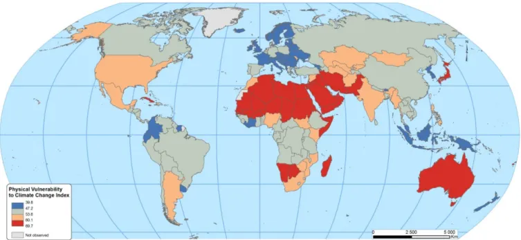
Figure.4 PVCCI on the map
5. Conclusion
The issue of climate change is a historical challenge of sustainable development. As often mentioned in the literature, the vulnerabilty to climate change is a complex concept which should be measured by relevant indicators, the relevance of which should be assessed with regard to their intended use. The conceptual framework of the vulnerability presented here is intended to be a useful tool for the allocation of resources devoted to the adaptation to climate change. It also intended to help in relative comparison of one country’s “physical” vulnerability to climate change to another by highlighting the factors that contribute to this vulnerability.
This paper proposes an index that captures the only physical vulnerability to climate change through its various manifestations in 191 countries around the world. The index differs from the abundant literature on vulnerability to climate change by considering only the part of vulnerability which does not depend on present or future country policy. To this aim, it relies only on physical components. These components are measured from observed trends in physical variables related to climate change and likely to have a socio-economic impact, but without any use of socioeconomic data. It is an index of physical or geo-physical vulnerability to climate change. It then differs from the more general environmental vulnerability indices, which include resilience and policy components, as well as environmental variables other than climate. It also differ from the Economic Vulnerability Index (EVI) used at the UN for the identification of the Least Developed Countries, related only to structural economic vulnerability covering the main kinds of external or natural exogenous shocks likely to affect economic growth.
The components of the PVCCI capture two types of risk related to climate change: the risks of an increase in the intensity of recurrent shocks (in temperature, rainfall, and storms), and the rather long term risks of progressive shocks (such as flooding due to higher sea level or desertification). The assessment of these risks relies on components referring both to the likely size of shocks and to the country’s exposure to these shocks. To adequately capture the specific vulnerability of each country, the components are averaged by using a quadratic average that enhances the impact of the component(s) reflecting the higher level of vulnerability.
The calculation of the index of physical vulnerability to climate change shows a higher average level for developing countries, in particular for SIDS,African countries and LDCs. However, based on their standard deviations, there is a wide disparity in PVCCI’s scores within these groups of countries. This higher physical vulnerability is in many countries amplified by a low structural resilence due to low level of income per capita and human capital
While the UN Economic Vulnerability Index (EVI) has been considered as a possible criterion for the
allocation of development assistance between developing countries (Guillaumont 2008,
Guillaumont et al., 2017), by the same way the PVCCI could be used as a criterion for the international allocation of the concessional resources devoted to the adaptation to climate change. It is a relevant criterion because it reflects the country needs for adaptation, independently of its policy. The two indices EVI and PVCCI can have a complementary role in the allocation of international resources, as far as these resources are provided from separate sources. The significant differences in ranking
between PVCCI and EVI supports the idea of two specific vulnerabilty based on assessments of “needs”.