Publisher’s version / Version de l'éditeur:
Earthquake Engineering and Structural Dynamics, 19, 3, pp. 359-376, 1990-04
READ THESE TERMS AND CONDITIONS CAREFULLY BEFORE USING THIS WEBSITE. https://nrc-publications.canada.ca/eng/copyright
Vous avez des questions? Nous pouvons vous aider. Pour communiquer directement avec un auteur, consultez la
première page de la revue dans laquelle son article a été publié afin de trouver ses coordonnées. Si vous n’arrivez pas à les repérer, communiquez avec nous à PublicationsArchive-ArchivesPublications@nrc-cnrc.gc.ca.
Questions? Contact the NRC Publications Archive team at
PublicationsArchive-ArchivesPublications@nrc-cnrc.gc.ca. If you wish to email the authors directly, please see the first page of the publication for their contact information.
NRC Publications Archive
Archives des publications du CNRC
This publication could be one of several versions: author’s original, accepted manuscript or the publisher’s version. / La version de cette publication peut être l’une des suivantes : la version prépublication de l’auteur, la version acceptée du manuscrit ou la version de l’éditeur.
Access and use of this website and the material on it are subject to the Terms and Conditions set forth at
Three-dimensional boundary element reservoir model for seismic
analysis of arch and gravity dams
Jablonski, A. M.; Humar, J. L.
https://publications-cnrc.canada.ca/fra/droits
L’accès à ce site Web et l’utilisation de son contenu sont assujettis aux conditions présentées dans le site LISEZ CES CONDITIONS ATTENTIVEMENT AVANT D’UTILISER CE SITE WEB.
NRC Publications Record / Notice d'Archives des publications de CNRC:
https://nrc-publications.canada.ca/eng/view/object/?id=d7ac4d6b-e9ca-4003-ae1b-93336c2049ba https://publications-cnrc.canada.ca/fra/voir/objet/?id=d7ac4d6b-e9ca-4003-ae1b-93336c2049baSer
TH1
N21 d National Research Conseil national no. 1664
1
C ouncll Canada de recherche$ Canadac,
2BLDG
Research in Institute for lnstitut de recherche en- Construction construction
Three-Dimensional Boundary Element
Reservoir Model for Seismic Analysis of
Arch and Gravity Dams
by A.M. Jablonski and J.L. Humar
Re~rinted from
~ a h h ~ u a k e Engineering and Structural Dynamics, Vol. 19, No. 3, April 1990 p. 354376
(IRC Paper No. 1664)
NRCC 31 733
-
N R C-
CIS^ dI W C
: . . '*,I
L I B R A R Y
, ? - ~ [ i r ;1;
! F ) ~ o 'La
m6thode &s Quatiom int6grales
a
6t6 utilish avec s u d s , dans le pas&, pour l'analyse
&s forces hydrodynamiques dans les dservoirs X i s
bidimensiomels ainsi que dans les
dservoirs finis bi- et tridimensiomels sounlis
A
des mouvements sismiques du
sol. Ce
document fait 6tat des resultat5 de recherches r6centes
concernant
l'application de
la
m6thode &s huations indgrales constantes h l'analyse 3D de la vibration &s
dservob.
On a i n c o r p d
B
cette
formulation &s conctitions limites spkiales, auparavanc utilides
dans le cas 2D,
afin
&
traiter l'amortissement
d6
aurayonnement f l m i
et
l'ammtissement
attribuable au sol de fondation et aux rives.
Les
auteurs pdsentent des donn6es
numCriques rendant compte & la vibration d'un
dservoi.
rectangulaire
infini
3D, ainsi
que
d'un
dservoir
infini
3D
f o n d
par
un
barrage-vofite, et ils
les
compmnt
il
c&s
r6sultats
obtenus
par
d'autres chercheurs.
EARTHQUAKE ENGINEERING AND STRUCTURAL DYNAMICS, VOL. 19, 359-376 (1990)
THREE-DIMENSIONAL BOUNDARY ELEMENT RESERVOIR
MODEL FOR SEISMIC ANALYSIS O F ARCH A N D
GRAVITY DAMS
A. M . JABLONSKIInstitute for Research in Construction, National Research Council, Ottawa, Canada K I A OR6 AND
J. L. HUMAR
Department of Civil Engineering, Carleton University, Ottawa, Canada K I S 6 8 6 SUMMARY
The boundary element method has been successfully applied in the past to the analysis of hydrodynamic forces in two- dimensional infinite as well as two- and three-dimensional finite reservoirs subjected to seismic ground motions. This paper presents the results of more recent research on the application of the constant boundary element method to the 3D analysis of reservoir vibration. Special boundary conditions, previously used in the 2D case, to treat infinite radiation damping and damping from foundation soil and banks have been incorporated in this formulation. Numerical results for vibration of a 3D infinite rectangular reservoir as well as of a 3D infinite reservoir impounded by an arch dam are presented and compared with some existing results obtained by other researchers.
INTRODUCTION
The seismic analysis and design of an arch dam has not been studied in as much detail as that of a concrete gravity dam because of the complex nature of the problem. The hydrodynamic forces caused by the vibration of the impounded water add to the complexity. Recently, closed form solutions have been developed by Porter and Chopra for the seismic vibrations of arch dam-reservoir systems of regular g e ~ m e t r y . ' ~ ~ For the systems of irregular geometry the finite element technique has been applied successfully. A three-dimensional model for the analysis of a gravity dam-reservoir-foundation system was first proposed by Hall and C h ~ p r a . ~ In this model the infinite water reservoir was divided into two parts: a finite irregular region and an infinite channel of constant cross-section. The finite element discretization was limited to the irregular region of the reservoir. For the infinite channel a two-dimensional finite element solution was employed. Compatibility of pressures and pressure gradients was then enforced at the interface of the regular and irregular regions of the reservoir to complete the solution.
Additional studies on the finite element analysis of arch dams have been carried out by Fok and C h ~ p r a . ~ - ' They developed an analytical procedure to account for both the effect of radiation damping and water reservoir-foundation interaction. The analysis of foundation interaction was based on a simplified model, first introduced by Hall and C h ~ p r a . ~
The considerable computational effort involved in the application of the FEM and the difficulty in modelling infinite domains have given impetus to studies based on the application of the boundary element method (BEM) to the response analysis of dam-reservoir-foundation systems. The boundary element method has been successfully applied to the analysis of hydrodynamic pressures in two-dimensional finite and infinite
reservoir^.'^-'^
The three-dimensional finite arch dam-reservoir vibration problem was solved by Elkhodary" using the direct boundary element method and by Humar and Jablonskilg using the so- called boundary element superposition method (BESM). The three-dimensional boundary element model has also been used by BiEkovskiZ0 in the treatment of seismic vibrations of a regular, rectangular, finite0
1990 by Government of Canada Received 14 July 1989360 A. M. JABLONSKI A N D J. L. HUMAR
reservoir. Soong and MurthaZ1 have recently reported the application of a three-dimensional boundary element model to the analysis of a dam-reservoir system.
This paper presents the results of the application of the boundary element method to the seismic analysis of a 3D infinite reservoir impounded by a simple arch dam.22 In a recent paper, Tsai and Lee23 have studied the hydrodynamic pressures in a 3D infinite reservoir based on a BEM model and omitting the far boundary. The present authors have found that the technique of omitting the far boundary is useful only for incompressible water or for excitation frequencies less than the first natural frequency of vibrations of the water reservoir. In the study reported here; the radiation damping due to outgoing waves in an infinite reservoir is accounted for by the application of a special boundary at the far end. This condition is similar to that developed earlier for finite element
solution^.^^^
The damping introduced by absorption of energy in a flexible foundation and banks is accounted for by another boundary condition originally developed by other researchers3Because BEM reduces the dimensionality of the problem by one, converting a three-dimensional domain problem to that of a surface, the discretization effort is considerably reduced. Thus BEM may serve as an effective alternative to FEM based procedures in the seismic analysis of a 3D dam-reservoir system. The objective of the present study was to demonstrate the effectiveness of BEM in modelling the reservoir. The dam was therefore treated as rigid. However, the procedure is extended easily to the case of a flexible dam. Additional work is required to develop the procedure into an effective tool for design. With this in view, conclusions and recommendations for future research are included.
ASSUMPTIONS
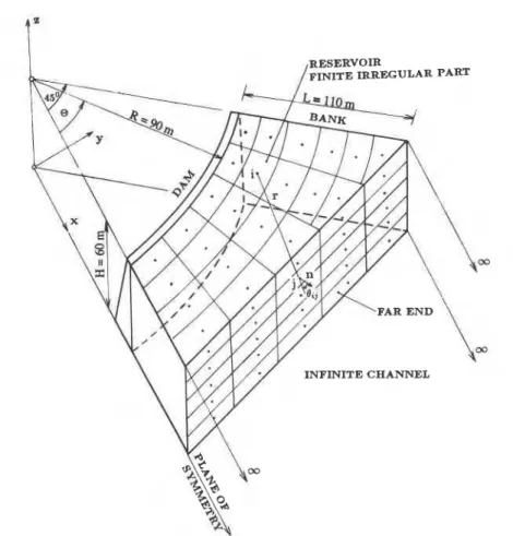
An arch dam-reservoir-foundation system consists of three parts: the dam, the impounded water reservoir, the foundation and banks (Figure 1). The arch dam is usually a curved thick shell (cylindrical, conical or paraboloidal). The ground motion to be considered in the analysis may be in any of the following three I directions: upstreamdownstream (x), cross-stream (y) and vertical (z).
It is assumed that, even though the ground motion varies with time, at any one instant it is identical throughout the reservoir bottom and banks.
The following assumptions are made in the derivation of the equations of motion for water in the 3D reservoir.
1. Water is compressible but non-viscous. 2. Effects of surface waves are negligible. 3. Only small amplitude motion is considered.
The reservoir may have a short length or may extend to a large distance. In the first case, the reservoir can be treated as finite; in the latter, it is considered to be infinite for the purpose of analysis.
EQUATIONS O F MOTION AND BOUNDARY CONDITIONS
Equations of motion
With the assumptions outlined in the foregoing paragraph the motion of the water in a 3D reservoir is governed by linearized Navier-Stokes equations. For a harmonic excitation ei"', these equations can be reduced to the known 3D Helmholtz equation
where x, y and z = the Cartesian coordinates shown in Figure 1; k = o / c is the wave number;
p
= pei"', the hydrodynamic pressure; o = the exciting frequency; and c = the velocity of sound in water.SEISMIC ANALYSIS OF ARCH A N D GRAVITY DAMS
Figure 1. Constant boundary element discretization of a 3 D finite reservoir impounded by an arch dam
Boundary conditions
The boundary conditions applicable to a general three-dimensional geometry are listed below. Along the dam-Jluid interface
a~
W- (s, r, o) = - -a,, (s, r )
an 9
where w = specific weight of water; s, r = coordinates over the dam-reservoir interface; a,@, r) = normal component of dam acceleration; n = outward normal to the interface.
Along the surface of the reservoir. Since the effect of surface waves is neglected, the hydrodynamic pressure should vanish at the free surface, giving
Along the reservoir bottom and banks. The boundary condition depends on whether the foundation is flexible or rigid. For a flexible foundation the boundary condition is derived from a simplified model in which one-dimensional seismic waves are assumed to propagate in a direction normal to the boundary and are reflected there. The detailed derivation has been presented by Hall and Chopra3 and leads to
a
P W-(st, r', o) = - -a,(sf, r') - i o y p(sl, r', o)
362 A. M. JABLONSKI AND J. L. HUMAR
where s', r' = coordinates over the reservoir bottom and banks; y = the damping coefficient; a,(sl, r') = the acceleration of the reservoir bottom and banks; w = the excitation frequency; and n = the outward normal to the reservoir bottom.
The second term on the R.H.S. of equation (4) represents the effect of foundation damping. The foundation damping coefficient is given by the following expression?
where a, = the coefficient of reflection. For a rigid foundation, a, = 1.0 and hence y = 0, while for full absorption a, = 0, y = llc.
The boundary condition along the banks is similar to that along the foundation.
Along the far boundary. For a 3D finite reservoir, the condition at the far end depends on whether that boundary is fixed or free to move. An infinite reservoir is modelled as consisting of two regions, a finite region which may be irregular, and an infinite channel of uniform cross-section. The interface between these two regions is called the far boundary or transmitting boundary. The energy loss due to radiation damping in the infinite region is accounted for through a special boundary condition similar to one used in the 2D
and based on that derived by Hall and C h ~ p r a . ~ In this derivation, the infinite channel of regular section is modelled by 2D finite elements along the interface cross-section with the variation in the longitudinal direction being represented by an exponentially decaying function. The problem ultimately reduces to the solution of a 2D eigenvalue problem. As an alternative a 2D boundary element representation can be employed to model the infinite channel. Details of the alternative procedure have been presented by K a n d a ~ a m y . ~ ~ The FEM discretization is used in the present case. Details of the derivation are similar to those in the 2D case and only a brief discussion of the eigenvalue problem is presented here.
The 3D Helmholtz equation [equation (I)] governs the vibration in the infinite channel as well, and can be solved by separation of variables:
in which p, satisfies the equation
and p,, satisfies the equation
where A2 = w2/c2
+
lcZ and lc is the separation constant.Equation (8) is solved by a two-dimensional finite element discretization. The FEM solution leads to the following eigenvalue problem:
where pyz is the vector of pressure values at nodes; and matrices A, B, F, d are obtained by assembling the corresponding element matrices. Details of the derivation may be found in References 3 and 22.
Equation (9) is valid for both horizontal excitations (downstream-upstream and cross-stream) and also for a vertical excitation, which is represented by the R.H.S. of that equation. Accordingly, the only non-zero terms in vector d are those corresponding to normal accelerations of the foundation and the banks.
SEISMIC ANALYSIS OF ARCH AND GRAVITY DAMS 363 Equation (10) represents an eigenvalue problem which for non-zero values of y leads to complex eigenvalues and eigenvectors. If the matrix of M eigenvectors obtained from equation (10) is represented by l , the following relationship must hold:
in which A = a diagonal matrix of the M eigenvalues A:, A;,
.
. . ,
I& (real or complex), and the eigenvectors have been normalized to be orthonormal w.r.t. F so thatFor a horizontal excitation the general solution for pressure vector p,, relating to the infinite region of the reservoir can be expressed in terms of computed eigenvalues 1, and eigenvectors
+,
asPyz = YEv (14)
in which y = a vector of modal coordinates, E = a diagonal matrix of terms e-""" and rc, =
,/-.
Differentiating equation (14) w.r.t. the outward normal to the finite part of the reservoir and noting that the normal is parallel to the x axis,
where K = a diagonal matrix with elements rc,, rc,,
. . .
, rcM, and q,, = apy,lan.For the case of vertical excitation, taking the origin at the far boundary (x = O), the vector of the nodal pressures can be expressed as
The total pressure is obtained by adding equations (14) and (16):
A modified mesh of the constant boundary elements at the transmitting boundary is required in order to match the boundary element pressure values with the nodal values of pressure in 4-node quadrilateral finite elements. This is discussed in a later section of this paper.
FORMULATION O F BOUNDARY ELEMENT EQUATIONS
For a numerical solution of the problem governed by equation (I), a weighted residual technique is used in which the governing equation is satisfied in an average sense over the domain V. Accordingly, equation (1) is multiplied by a weighting function p* and the integral of the product over the domain is equated to zero. Repeated partial integration and the application of Green's theorem, leads to the following boundary integral equation:l5- 2 2
364 A. M. JABLONSKI A N D J. L. HUMAR
The R.H.S. of equation (18) contains surface integrals over the boundary S only while the L.H.S. contains a
volume integral. By an appropriate choice of the function p*, the integration over domain Vmay be avoided. The desired weighting function p* is chosen to satisfy the following equation:
in which A' = a Dirac delta function centred at point i having coordinates (xi, yi, zi).
The solution of equation (19) is called the fundamental solution. It can be obtained by the so-called Green's function a p p r o a ~ h l ~ , ~ ~ , ~ ~ and is given by
where r = the radial distance given by r = ,/(x -
+
(y - yi)2+
(Z - z ~ ) ~ , and the point with the coordinates (xi, y,, zi) is referred to as the source point.Other possibilities exist for the selection of a fundamental solution. For example, Tsai and Lee23 have used the following fundamental solution which satisfies implicitly the free surface condition:
where r' = the distance between the field point and the mirror image point. Research on the most appropriate and effective fundamental solution for both 2D and 3D cases is still continuing.17723
Substitution of equation (19) into equation (18) gives
in which ci = 1 for a point inside the water reservoir, ci =
3
for a point on the smooth boundary of the water reservoir, ci = 0 for a point outside the water reservoir, pi = the hydrodynamic pressure at point i, q = aplan and q* = ap*/an. The subscripts on pf and qf indicate that the latter are produced by a source at point i.Equation (22) provides a means of determining the unknown pressure at point i within the domain in terms of the integrals of pressure and pressure derivative values on the boundary. While some of these values are specified, others must be determined before equation (22) can be used. In a boundary element formulation, equation (22) itself is used to determine the unknowns on the boundary. To achieve this the boundary surface is divided into a series of elements and the parameters p and q are assumed to vary in a prescribed manner over a given element.
For example, in a 2D case, individual elements are straight lines and the pressure and pressure derivatives may be assumed to be constant over an element, leading to the so-called constant boundary element formulation. As an alternative, the parameters p and q may be assumed to vary linearly over an element. They are expressed as linear functions of the p and q values at the end points of the element. This gives a linear element formulation. In fact, the variation may be expressed as a superposition of shape functions of a coordinate along the boundary, each function being weighted by a nodal parameter. These nodal parameters become the unknowns in the formulation. This procedure is exactly parallel to the shape function approach need in the FEM.
In the present work, the boundary elements are quadrilaterals and p and q are assumed to be constant over an element and equal to their values at the midpoints of the element. Boundary elements of this type are referred to as constant elements. Investigations conducted by the authors for the 2D showed that the constant boundary elements were quite effective and that acceptable accuracy was achieved with a reasonable number of such elements.
SEISMIC ANALYSIS OF ARCH A N D GRAVITY DAMS 365 The constant boundary element formulation for the three-dimensional Helmholtz equation has previously been used by Elkhodary18 in his analysis of the 3D finite reservoir subjected to small harmonic vibrations. Therefore only the essential points of the derivation are presented in this paper.
Equation (22) for a given point i on the boundary S has the following discretized form:
where pj and q j are the pressure and pressure gradient, respectively, over the centre of the jth element and are assumed to be constant over that element, while Sj represents the surface of the element.
A constant boundary element model of the three-dimensional infinite water reservoir is presented in Figure 1.
Equation (23) can be also expressed in a matrix form as follows:
where p and q are respectively the vectors of N unknown pressures and pressure derivatives at the boundary element nodes; and H and G are matrices of order N whose elements are given by
Defining a local coordinate system
5,
andt2
and using a Gauss quadrature formula for evaluating the integrals, an expression for Hij is obtained in the following form:1 4 H = -
2
( )
[(cos kr+
kr sin kr)+
i( - sin kr+
kr cos kr)Lm Ill on.lJ 47Cn=lm=l a m (26)
where on, = weighting function used in the Gauss quadrature;
I
JI = the Jacobian of transformation between the (x, y, z) coordinates system and the ( t , , 5,) local coordinates system; and 8 = the angle between the outward normal n and the radius vector r, as shown in Figure 1. When i = j equation (26) reduces toH.. = -
'
2.The term Gij is also determined by a numerical integration and is given by
The term Gii is calculated by excluding the singular point i. Details have been presented by Elkhodary." INCORPORATION O F INFINITE RADIATION CONDITION AND DAMPING ALONG
FOUNDATION AND BANKS
To match the solution at the interface of the finite and infinite region, and to apply the condition along the reservoir bottom and banks, equation (24) is expressed in a partitioned matrix form as follows:~
366 A. M. JABLONSKI A N D J. L. HUMAR
in which p,, q, represent, respectively, the pressures and pressure derivatives at the nodes on the reservoir surface and along the dam face, p,, q2 represent the same quantities on the reservoir bottom and banks, while p,, q3 represent them at the nodes on the transmitting boundary.
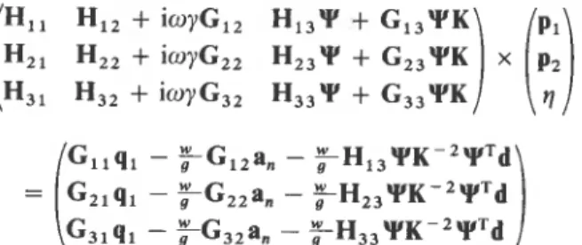
When a constant boundary element formulation is used in the 3D infinite case, difficulty arises in the evaluation of p,, because, while the finite element nodes are located at the vertices of a 4-node quadrilateral element, the constant boundary element nodes are at the geometric centres of these elements. One possible way to resolve it is to use different meshes for the boundary discretization and the finite element discretization. By proper selection of the meshes it is possible to match most of the nodes in the two formulations. An example of such a mesh division is presented here in Figure 2. Nodes 6, 7, 10 and 11 are identical in two meshes. Nodes 1 to 4,5,8,9,12 and 13 to 16 do not match exactly, but the p and q values for the BEM and FEM sets are assumed to be identical. Also the pressure at nodes 4,8, 12 and 16 is assumed to be zero in both cases. Using equations (4), (15) and (17) equation (28) can be expressed as
Equation (29) represents the constant boundary element formulation for the 3D case, including the infinite radiation condition and damping along the foundation and banks. It contains N unknown values of p, q and q.
ANALYTICAL RESULTS
A computer program was developed to calculate the hydrodynamic pressures in a 3D reservoir due to prescribed excitation of the dam face and reservoir bottom and banks. The program uses the constant boundary elements. An infinite reservoir is divided into the two previously described regions, one irregular but finite and the other in the form of an infinite channel of constant cross-section. The eigenvalue problem associated with the infinite region is solved by two-dimensional finite element discretization using the QZ algorithm originally developed by Moler and Stewart.27
Selected results of analytical studies carried out by using the formulation and the computer program mentioned in the preceding paragraphs are presented here. A BEM model of the three-dimensional rectangular reservoir is considered first in order to compare the analytical results with classical results obtained from a corresponding 2D model. A 3D reservoir impounded by a circular arch dam is considered next.
isoparametric finite element nodes
\2 \>Is
!
10;2
4
10,~"":midnodes of the
SEISMIC ANALYSIS OF ARCH A N D GRAVITY DAMS 367
Rectangular three-dimensional infinite reservoir
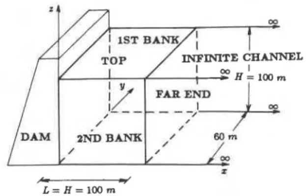
The rectangular reservoir studied is shown in Figure 3. The following data are used in the computations: height of the reservoir, H = 100 m; velocity of sound in water, c = 1440 m/s; the mass density of water,
p = 1 tonne/m3. For the data given, the fundamental frequency of the reservoir o, = .nc/2H becomes
22.62 rad/s (3.6 Hz). The transmitting boundary is placed at a distance of 100 m from the upstream dam face. The constant boundary element model of the reservoir being studied consists of 119 boundary elements. In the finite element model of the infinite channel, 15 4-node linear isoparametric quadrilateral elements are used.
The results presented here show the variations of hydrodynamic pressure along the dam face for two types of harmonic motion: upstream4ownstream and vertical motion. Four different foundation damping levels are considered with the following values of coefficient of reflection: a, = 0.0, 0.5, 0.75 and 1.0, the last one corresponding to full reflection or the rigid case.
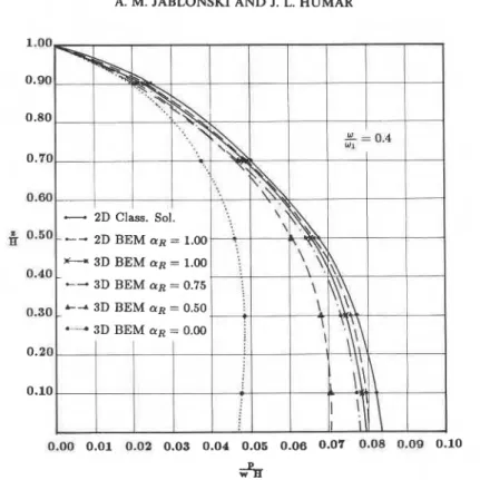
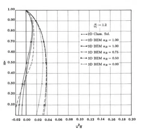
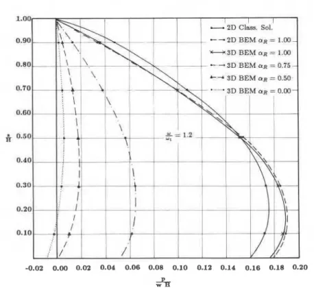
The results for upstream-downstream harmonic motion are presented in Figures 4 and 5. The real and imaginary components of the hydrodynamic pressure are shown separately. Results are presented for two excitation frequencies given by o/w, = 0.4 and 1.2. The results for a rigid case (a, = 1.0) show very good agreement with 2D classical3 and BEM results,15 especially for o
<
o , . In this case, the imaginary part of the hydrodynamic pressure is negligible; theoretically it ought to be zero. For o > o, (o/o, = 1.2), the imaginary part is predominant. The results for a rigid case (a, = 1.0) are still in reasonably good agreement with 2D classical3 and BEM solutions.22 In both cases, the introduction of damping results in a decrease in the response. Evidently the decrease is most significant for a, = 0 (full damping case).The results for vertical harmonic motion are presented in Figure 6. The real and imaginary parts of the hydrodynamic pressure are shown separately. Results are presented for an excitation frequency o = 1.20,. Four different levels of damping with coefficient of reflection values of 1.0 (rigid case), 0.75,O-50 and 0.0 (full damping case) are considered. Again, the results for a rigid case are in good agreement with the 2D classical and BEM
result^.^^
2 2 Introduction of damping results in a decrease in the response. The good comparisonbetween the 3D BEM results and the 2D classical and BEM results provides a partial verification of the formulation and the computer algorithm.
Three-dimensional reservoir impounded by an arch dam
Results of analytical studies of hydrodynamic pressures in a 3D infinite reservoir impounded by a circular arch dam are presented next. The effects of infinite radiation damping and foundation and banks damping are also considered. The following data are used in the computation: height of the reservoir, H = 60 m; radius of the circular section of the arch dam, R = 90 m; length of the finite part of the reservoir, L = 110 m; velocity of sound in water, c = 1440 m/s; the mass density of water, p = 1 tonne/m3. Beyond L = 110 m the reservoir is represented by an infinite channel of rectangular cross-section. For the given data the fundamental frequency of the reservoir o, = nc/2H becomes 37.7 rad/s (6 Hz).
A. M. JABLONSKI A N D J. L. HUMAR
Figure qa). Real part of
-
2D Class. Sol.- ' > N
1
1
1
--
2D BEM a~ = 1.00 , I \ ' . '---a 3D BEM a~ = 0.00 j I 0.20 0.10the hydrodynamic pressure on a gravity dam due to upstream-downstream harmonic motion in a 3 D infinite
rectangular reservoir-+lo, = 0 4
Figure qb). Imaginary part of the hydrodynamic pressure on a gravity dam due to upstream-downstream harmonic motion in a 3D
SEISMIC ANALYSIS OF ARCH AND GRAVITY DAMS
Figure 5(a). Real part of the hydrodynamic pressure on a gravity dam due to upstream-downstream harmonic motion in a 3D infinite rectangular reservoir--w/w, = 1.2
Figure 5(b). Imaginary part of the hydrodynamic pressure on a gravity dam due to upstream-downstream harmonic motion in a 3 D infinite rectangular reservoir--o/o, = 1.2
A. M. JABLONSKI AND J. L. HUMAR
Figure qa). Real part of the hydrodynamic pressure on a gravity dam due to vertical harmonic motion in a 3D infinite rectangular reservoir--o/w, = 1.2
Figure 6(b). Imaginary part of the hydrodynamic pressure on a gravity dam due to vertical harmonic motion in a 3D infinite rectangular reservoir+/o, = 1.2
SEISMIC ANALYSIS OF ARCH A N D GRAVITY DAMS 37 1
The constant boundary element model of the reservoir consists of 260 4-node constant quadrilateral boundary elements. In addition 30 Cnode linear isoparametric quadrilateral finite elements are used to model the infinite channel.
The results presented here show the variation of hydrodynamic pressure along the upstream dam face for three types of harmonic motion: upstream-downstream, cross-stream and vertical motion.
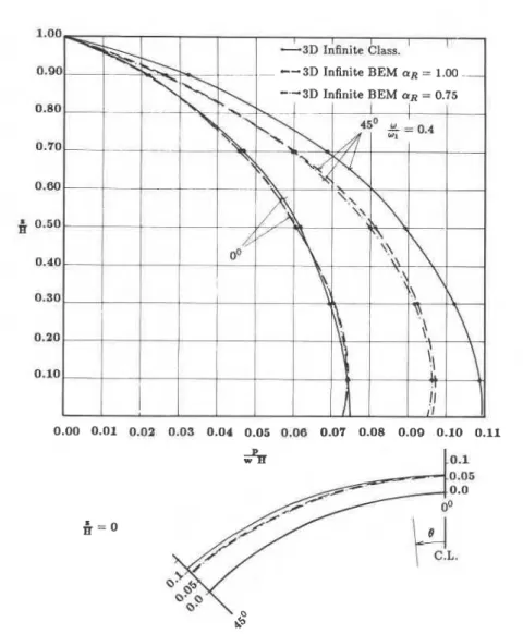
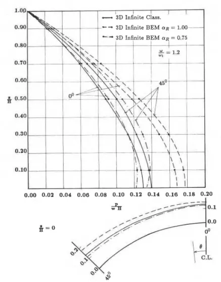
The results for upstream-downstream harmonic motion are presented in Figures 7 and 8 for o/o, = 0.4 and o/o, = 1.2 respectively. Two different values of coefficient of reflection a, = 0.75 (25 per cent absorption) and a, = 1.0 (full reflection, rigid case) are considered. The 3D classical results obtained by Porter and C h ~ p r a ' , ~ for a radially infinite reservoir are also shown for comparison. The classical results should be compared with the 3D BEM results for a rigid case, a, = 1.0. Most of the results show qualitative similarity in the two sets of response; however, significant differences exist, presumably because of the difference in the geometry of the infinite part. The classical solution is based on radial banks while in the BEM solution the banks in the infinite channel are parallel to the x axis.
Figure 7. Absolute value of the hydrodynamic pressure on an arch dam due to upstream4ownstream harmonicmotion in a 3D infinite reservoir--o/w, = 0.4
1.00 0 . w 0.80 0.70 0.m
6
0.50 0.40 0.30 0.20 0.10 0.00 0.02 0.04 0.06 0.08 0.10 0.12 0.14 0.16 0.18 0.20Figure 8. Absolute value of the hydrodynamic pressure on an arch dam due to upstream-domstream harmonic motion in a 3D infinite reservoir--o/o, = 1.2
1.00 0.90 0.80 0.70 0.60 5 0.50 H ? 0.40
ic
*G
0.305
5
0.20E
%
'3 0.10 ;I
11n
*
r
8
i! Z C 0.00 0.01 0.02 0.03 0.04 0.05 0.06 0.07 0.08 0.09 0.105
-
0.05 w8
= 0 oyFigure 9. Absolute value of the hydrodynamic pressure on an arch dam due to cross- stream harmonic motion in a 3D infinite reservoir--o/o, = 0.4
A. M. JABLONSKI AND J. L. HUMAR
<r
--."
Q!+ C.L.
I
0'
Figure 12. Absolute value of the hydrodynamic pressure on an arch dam due to vertical harmonic motion in a 3D infinite reservoir-
w / w , = 1.2
The results of the analysis for cross-stream harmonic motion are presented in Figures 9 and 10 for o/w,
= 0.4 and w/o, = 1.2 respectively. The results of 3D BEM are different from the classical infinite case reported by Porter and C h ~ p r a . ' , ~ Apparently, the geometry of the infinite part of the reservoir has a significant influence on the results.
Finally the hydrodynamic pressures due to a vertical harmonic motion are presented in Figures 11 and 12 for o/o, = 0 4 and w/o, = 1.2 respectively. For o < w, ( o = 0.4 o , ) the results of BEM analysis are quite close to the classical s ~ l u t i o n . ' , ~ Evidently, the difference in the geometry of the infinite channel does not affect the results. For o > w, ( o = 1.2~0,) the two sets of results are different even though a qualitative similarity exists. In this case the difference in the geometry of the infinite channel has a pronounced effect.
SUMMARY AND CONCLUSIONS
This paper describes the boundary element technique for the linear analysis of hydrodynamic pressures in a 3D reservoir for a harmonic motion of the dam and/or the reservoir bottom and banks. The constant boundary element formulation is used. The energy loss in the waves travelling to infinity is represented by a
SEISMIC ANALYSIS O F ARCH AND GRAVITY DAMS 375
special boundary condition to be applied to the truncated far end of the reservoir (transmitting boundary). This boundary condition has been successfully used in a finite element analysis and also in a 2D boundary element analysis of dam-reservoir systems. In addition, a special foundation damping condition developed by other researchers for an FEM analysis has been incorporated in the BEM formulation presented here. Although the results presented are for harmonic motion only, the analytical procedure can be extended easily to the case of the random earthquake motion by using the fast Fourier transformation technique.
Several observations can be made as a result of the present research.
1. The boundary element method (BEM) is an effective procedure for evaluating hydrodynamic pressures in a 3D water reservoir of arbitrary shape.
2. When compared to the finite element method (FEM), BEM offers the advantage of reducing the dimensionality of the problem by one.
3. In comparison to the 2D case, the fundamental solution for a 3D BEM formulation is of simpler nature. 4. The analysis of a flexible dam for an arbitrary ground motion taking into account the foundation-dam
interaction can be achieved by a substructuring technique in which the dam is discretized by FEM or BEM and the reservoir is modelled by BEM.
5. A drawback of the BEM is the frequency dependence of the fundamental solution which requires the
computation of the elements of boundary element matrices for each excitation frequency. The use of a frequency independent fundamental solution is therefore of interest and needs to be pursued.
6. The effect of the location of the far end transmitting boundary needs additional studies.
7. The effect of damping introduced by a flexible foundation and banks could be evaluated by a more detailed representation using the BEM to model a semi-infinite medium and coupling the model with that for the reservoir.
ACKNOWLEDGEMENT
The research reported here was supported by a grant from the Natural Science and Engineering Research Council, Canada.
REFERENCES
1. C. S. Porter and A. K. Chopra, 'Dynamic response of simple arch dams including hydrodynamic interaction', Report No. UCBIEERC-80117, Earthquake Engineering Research Center, University of California, Berkeley, CA, 1980.
2. C. S. Porter and A. K. Chopra, 'Hydrodynamic effects in dynamic response of simple arch dams', Earthquake eng. struct. dyn. 10,
417-431 (1982).
3. J. F. Hall and A. K. Chopra, 'Dynamic response of embankment concrete gravity and arch dams including hydrodynamic interaction', Report No. UCBJEERC-80139, Earthquake Engineering Research Center, University of California, Berkeley, CA, 1980.
4. K. L. Fok and A. K. Chopra, 'Earthquake analysis and response ofconcrete arch dams', Report No. UCBIEERC-85/07, Earthquake Engineering Research Center, University of California, Berkeley, CA, 1985.
5. K. L. Fok and A. K. Chopra, 'Earthquake analysis of arch dams including dam-water interaction', Earthquake eng. struct. dyn. 14,
155-184 (1986).
6. K. L. Fok and A. K. Chopra, 'Hydrodynamic and foundation flexibility effects in earthquake response of arch dams', J. struct. div. ASCE 112, 181G1828 (1986).
7. K. L. Fok and A. K. Chopra. 'Frequency response functions for arch dams: Hydrodynamic and foundation flexibility effects', Earthquake eng, srnrct. iiyn. 14. 769-795 (1986).
8. K. L. Fok and A. K. Chopra. 'Water compressibility in earthquake response of arch dams', J. struct. div. ASCE 113,958-975 (1987). 9. K. L. Fok. J. F. Hall and k K. Chopra. 'EACD-3D: A computer program for three-dimensional earthquake analysis of concrete
dams'. Repon No. UCU!EERC-86!09, Earthquake Engineering Research Center, University of California, Berkeley, CA, 1986.
10. Y. G. Hanna, 'Application of b o u n d a ~ element method to mrtain problems in structural dynamics', M. Eng. Thesis, Carleton Univeristy, Ottawa. Canada 1980.
11. Y. G. Manna and I. L. Hurnar, 'Boundary element analysis o f fluid domain', J. eng. mech. diu. ASCE 108, 436450 (1982). 12. P. L.-F. Liu and A. H.-D. Cheng, 'Boundary solutions for fluid-structure interaction', J. hydr. eng. div. ASCE 110, 5 1 4 4 (1984). 13. P. L.-F. Liu, 'Hydrorlynamic pressures on rigid dams during earthquakes', J.Jluid mech., 165, 131-145 (1986).
14. J. L. Hurnar and A. M. Jablonski, 'Boundary element analysis of the hydrodynamic forces in a 2D reservoir', Proc. 5th Can. con! earrhquokr prig. Ottawa. Canada (1987).
15. 1. L. Humar and A. M. Jablonuki, 'Boundary element reservoir model for seismic analysis of gravity dams', Earthquake eng. struct. dyn. 16: 1 129-1 156 (1988).
16. D. H. Wepf and J. P. Wolf, 'Time domain dam-reservoir interaction analysis based on boundary elements', Proc. China-U.S.A. workshop on earthquake behaviour of arch dams Bejing, China (1987).
376 A. M. JABLONSKI AND J. L. HUMAR
17. D. H. Wepf, J. P. Wolf and H. Bachmann, 'Hydrodynamic-stiffness matrix based on boundary elements for time-domain dam-reservoir-soil analysis', Earthquake eng. struct. dyn. 16, 417432 (1988).
18. M. A. Elkhodary, 'Boundary element analysis of hydrodynamic pressure on arch dams', M . Eng. Thesis, Carleton University, Ottawa, Canada, 1984.
19. J. L. Humar and A. M. Jablonski, 'Boundary element superposition analysis of reservoir motion', Proc. 8th Eur. con$ earthquake eng. Lisbon, Portugal (1986).
20. V. BiEkovski. 'Mathematical modelling of arch dams under high seismicity conditions', Proc. 8th Eur. con$ earthquake eng. Lisbon,
Portugal (19'86).
-
21. T. W. Soong and J. P. Murtha, 'Boundary integral equation approach to earthquake induced hydrodynamic forces', Proc. 5th c o n !
comput. civil eng.: microcomputers to supercomputers Alexandria, Virginia (1988).
22. A. M. Jablonski, 'Boundary element analysis of earthquake induced hydrodynamic pressures in a water reservoir', Ph.D. Thesis, Carleton University, 1988.
23. C. S. Tsai and G. C. Lee. 'Arch dam-fluid interaction by BEM-FEM and substructure concepts', Int. j. numer. methods eng. 24,
2367-2388 (1987).
24. K. Kandasamy, 'Three-dimensional dynamic analysis of gravity dam and reservoir system', Ph.D. Thesis, John Hopkins University, Baltimore, Maryland, 1986.
25. M. D. Greenberg, Application of Green's Function in Science and Engineering, Prentice-Hall, Englewood Cliffs, New Jersey, 1971. 26. R. E. Collins, Mathematical Methods for Physicists and Engineers, Reinhold Physics Textbook Series, Reinhold Book Corp., New
York, 1968.