Learning spatiotemporal piecewise-geodesic trajectories from longitudinal manifold-valued data

(1)

HAL Id: hal-01646617

https://hal.archives-ouvertes.fr/hal-01646617v2

Submitted on 12 Dec 2017

HAL is a multi-disciplinary open access

archive for the deposit and dissemination of

sci-entific research documents, whether they are

pub-lished or not. The documents may come from

teaching and research institutions in France or

abroad, or from public or private research centers.

L’archive ouverte pluridisciplinaire HAL, est

destinée au dépôt et à la diffusion de documents

scientifiques de niveau recherche, publiés ou non,

émanant des établissements d’enseignement et de

recherche français ou étrangers, des laboratoires

publics ou privés.

Learning spatiotemporal piecewise-geodesic trajectories

from longitudinal manifold-valued data

Juliette Chevallier, Stéphane Oudard, Stéphanie Allassonnière

To cite this version:

Juliette Chevallier, Stéphane Oudard, Stéphanie Allassonnière. Learning spatiotemporal

piecewise-geodesic trajectories from longitudinal manifold-valued data. Neural Information Processing Systems

2017, Dec 2017, Long Beach, CA, United States. �hal-01646617v2�

(2)

Learning spatiotemporal piecewise-geodesic trajectories

from longitudinal manifold-valued data

Juliette Chevallier, Stéphane Oudard and Stéphanie Allassonnière

CMAP, École polytechnique – Oncology departement, HEGP – CRC, Université Paris Descartes

Overview

We introduce a hierarchical model which allows to estimate both a group-representative piecewise-geodesic trajectory in the Riemannian space of shape and inter-individual variability. Following the approach of [3], we estimate a representative

piecewise-geodesic trajectory of the global

pro-gression and together with spacial and temporal

inter-individual variabilities. We first introduce

our model in its most generic formulation and then make it explicit for recist [4] score monitoring, i.e. for one-dimension manifolds and piecewise-logistically distributed data.

Medical context – RECIST score

•New anti-angiogenic therapies. Patients suffering from the metastatic kidney cancer take a drug each day [1];

•Tumoral growth. The recist score (response evalua-tion criteria in solid tumors) is a set of published rules that measures the tumoral growth;

•Patient’s response. The response to a given treatment has generally two distinct phases: first, tumor’s size re-duces; then, the tumor grows again;

•Moreover, a practical question is to quantify the corre-lation between both phases and to accurately determine when the patient’s response escape to treatment.

0 50 100 150 200 250 300 350 400 450 500 0 50 100 150 200 250 300 350 400 450 “0 “1 “2 “3 “4 “5 “6 “7 “8

Time (in days)

REC IS T sco re (d imen tio nl ess)

Figure 1:After 600 iterations. First 8 patients among the 176

Longitudinal dataset: Given n œ Nú_{individuals and}

(ki)iœJ1,nK, we observe the sequences t = (ti,j)jiœœJJ1,n1,kKiKœ R

k and y = (yi,j)i_jœ_œJ_J1,n1,kKiKœ R

kd_{where k =}Pn i=1ki.

Data points are seen as noisy samples along trajectories. Real data consists of recist scores of a drove of 176 patients of the hegp, with an average of 7 visits per subjects (min:3, max:22).

Mixed-effects model for piecewise-geodesically distributed data

Group-representative trajectory “0. Given m œ

Nú_{and t}_R₌⇣_{≠Œ < t}1

R< . . . < tmR≠1<+Œ

⌘

, we build “0in order it to be geodesic on each ]t¸R≠1, t¸R].

1Let M0 µ Rd _{a geodesically complete manifold,}

⇣

¯“¸ 0

⌘

¸œJ1,mKa family of geodesics on M0and ⇣

„¸ 0

⌘

¸œJ1,mK

a family of isometries defined on M0;

2’¸ œJ1, mKwe set M0¸= „0¸(M0) and “¸0= „¸0¶ ¯“¸0;

3A piecewise-geodesic curve. We define “0as “0= “011]≠Œ,t1 R]+ m_X_X_X≠1 ¸=2 “¸ 01]t¸≠1 R ,t¸R]+ “ m 0 1]tm≠1 R ,+Œ[;

4Boundary conditions. We impose boundary conditions

on the rupture times to ensure continuity.

Individual trajectories (“i)iœJ1,nK. Let i œ J1, nK.

We build “i to derive from “0 through spatiotemporal transformations.

1Time warps (Â¸_i)_¸_œ_J1,mK. We choose affine time warps

constrains by the continuity of each individual paths;

2Space warps („¸_i)_¸_œ_J1,mKhave to be defined in view of

applications. We require „¸ i¶ “0¸(t¸R) = „i¸+1¶ “0¸+1(t¸R) ; 3Last, ’¸ œJ1, mKwe set “_i¸= „¸_i¶ “¸ 0¶ Âi¸and “i= “i11]≠Œ,t1 R,i]+ m_X_X_X≠1 ¸=2“ ¸ i1]t¸≠1 R,i,t¸R,i]+“ m i 1]tm≠1 R,i,+Œ[;

4Gaussian noise. ’j œJ1, kiK, yi,j= “i(ti,j) + Ái,jwhere Ái,j≥ N (0, ‡2), ‡ œ R+.

Chemotherapy monitoring: Piecewise-logistic curve model

“init_{0 ≠‹} “escap₀ +‹ “fin0 ≠‹ eﬂ1i eﬂ2i ”i ·i t0 ti R ti tR t1 1 “0 “i

Figure 2:From average to individual path. Boundary conditions

and transition from “0to “ithrough spacial and temporal warps. zpop=⇣“0init, “0escap, “0fin, tR, t1

⌘

and zi= (›i1, ›i2, ·i, ﬂ1i, ﬂ2i, ”i).

Our observations consist of patient’s recist score over time. So, we set m = 2, d = 1 and M0= ]0, 1[ equipped with the logistic metric. Let ‹ œ R and i œJ1, nK.

•Representative trajectory “0. Let “init0 , “0escap, “fin0 œ R. We map M0onto ]“escap

0 , “0init[ and ]“escap0 , “0fin[ through affine transformations and require that “1

0(t0) = “init0 ≠‹, “01(tR) = “02(tR) = “escap0 + ‹ and “20(t1) = “0fin≠ ‹ ;

•Time warps (Â1

i, Â2i). We set –¸i= e›

¸

i, ¸ œ {1, 2} ;

•Space warps („1

i, „2i). Given (ﬂ1i, ﬂ2i, ”i) œ R3, we set „¸

i: x ‘æ eﬂ

¸

i(x ≠ “0(t_R)) + “0(t_R) + ”_i, ¸ œ {1, 2} .

Parameters estimation with the MCMC-SAEM algorithm

Existence of the MAP

Given the piecewise-geodesic model and the choice of probability distributions for the parameters and latent variables of the model, for any dataset (t, y), there exists_{◊M AP}b _{œ argmax}

◊œ q(◊|y).

•Parameters. We assume that zpop ≥ N (zpop, pop) where pop is a diagonal matrix with small fixed en-tries [2] and that zi≥ N (0, ) where œ S6(R). Let ◊=⇣“init0 , “0escap, “fin0, tR, t1, , ‡

⌘

;

•Hierarchical model. Let z = (zpop, zi)iœJ1,nK. We have 8 > > > > > > > > > < > > > > > > > > > : y| z, ◊ ≥ On i=1 ki O j=1 N⇣“i(ti,j), ‡2 ⌘ z| ◊ ≥ N (zpop, pop)On i=1 N (0, ) ( , ‡) ≥ W≠1_{(V, m ) ¢ W}≠1_{(v, m} ‡) where V œ S6(R) and v, m , m‡œ R ;

•Estimation. We use a symmetric random walk

Hastings-Metropolis sampler in a stochastic version of the em algorithm.

Experimental results

Synthetic data. Experiments are performed for the

piecewise-logistic model.

Table 1:Mean (standard deviation) of relative error (expressed as a percentage) for the population parameters zpopand the residual

standard deviation ‡ for 50 runs according to the sample size n.

n 50 100 150 “init₀ 1.63 (1.46) 2.42 (1.50) 2.14 (1.17) “escap₀ 9.45 (5.40) 9.07 (5.19) 11.40 (5.72) “₀fin 6.23 (2.25) 7.82 (2.43) 5.82 (2.55) tR 11.58 (1.64) 13.62 (1.31) 9.24 (1.63) t1 4.41 (0.75) 5.27 (0.60) 3.42 (0.71) ‡ 25.24 (12.84) 10.35 (3.96) 2.83 (2.31)

Real data. Figure 1 illustrates the qualitative

perfor-mance of the model on the first 8 patients.

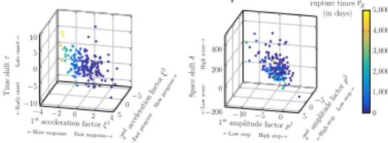
2 ndac celer ation factor › 2 ΩFa stpr ogress Slow prog ressæ 1st_{acceleration factor ›}₁ ΩSlow_{response Fast responseæ}

Tim e shift · Ω E ar ly ons et La te ons et æ ≠4 ≠2 0 2 4 ≠5 0 5 ≠10 ≠5 0 5 10 ≠10 ≠5 0 ≠5 0 5 ≠200 0 200 400 0 1,000 2,000 3,000 4,000 5,000 2 ndam plitude factor ﬂ 2 ΩHig hste pLo wste pæ 1st_{amplitude factor ﬂ}1 ΩLowstep High stepæ

Spac e shift ” Ω Lo w sc or e Hig h sc or eæ Individual rupture times ti R (in days)

Figure 3:Individual random effects. Figure 3a: ›1

iand ›i2against ·i.

Figure 3b: ﬂ1

iand ﬂ2iagainst ”i. In both figure, the color corresponds

to the individual rupture time ti R. 0 500 1,000 1,500 2,000 2,500 3,000 3,500 4,000 4,500 5,000 0 10 20 30 40 50

Individual rupture times (in days)

Figure 4:Distribution of the individual rupture times ti_{R. In black}

bold line, the estimated average rupture time tR.

References

[1] Escudier, Porta, Schmidinger, Rioux-Leclercq, Bex, Khoo, Gruenvald, and Horwich, Renal

cell carcinoma: Esmo clinical practice guidelines for diagnosis, treatment and follow-up,

Annals of Oncology 27 (2016), no. suppl 5, v58–v68.

[2] Kuhn and Lavielle, Maximum likelihood estimation in nonlinear mixed effects models, Computational Statistics & Data Analysis 49 (2005), no. 4, 1020–1038.

[3] Schiratti, Allassonniere, Colliot, and Durrleman, Learning spatiotemporal trajectories from

manifold-valued longitudinal data, Neural Information Processing Systems 28, 2015.

[4] Therasse, Arbuck, Eisenhauer, Wanders, Kaplan, Rubinstein, Verweij, Van Glabbeke, van Oosterom, Christian, and Gwyther, New guidelines to evaluate the response to treatment

in solid tumors, Journal of the National Cancer Institute 92 (2000), no. 3, 205–216. Acknowledgements

This work was supported by the French public grant Investissement d’Avenir, project anr-11 lbx-0056-lmh, and the Foundation of Medical Research, project dbi20131228564.