HAL Id: hal-01383118
https://hal.inria.fr/hal-01383118
Submitted on 18 Oct 2016HAL is a multi-disciplinary open access archive for the deposit and dissemination of sci-entific research documents, whether they are pub-lished or not. The documents may come from teaching and research institutions in France or abroad, or from public or private research centers.
L’archive ouverte pluridisciplinaire HAL, est destinée au dépôt et à la diffusion de documents scientifiques de niveau recherche, publiés ou non, émanant des établissements d’enseignement et de recherche français ou étrangers, des laboratoires publics ou privés.
competition during tri-stable motion perception
Andrew Meso, James Rankin, Olivier Faugeras, Pierre Kornprobst, Guillaume
Masson
To cite this version:
Andrew Meso, James Rankin, Olivier Faugeras, Pierre Kornprobst, Guillaume Masson. The relative contribution of noise and adaptation to competition during tri-stable motion perception. Journal of Vision, Association for Research in Vision and Ophthalmology, 2016. �hal-01383118�
The relative contribution of noise and adaptation to competition
during tri-stable motion perception
Andrew Isaac MESOa,d*, James RANKINb,c, Olivier FAUGERASb,
Pierre KORNPROBSTe, Guillaume S MASSONa
Adresses:
a Institut de Neurosciences de la Timone
UMR 7289 CNRS & Aix-Marseille Université 27 Bd Jean Moulin
13385 Marseille Cedex 05, France
b Université Côte d'Azur
Inria Sophia Antipolis Méditerannée Team Mathneuro
Routes des Lucioles – BP 93, Sophia Antipolis 06902, France
c Center for Neural Science,
New York University 4 Washington Place, New York, NY 10003
d Psychology and Interdisciplinary Neurosciences Research Group,
Faculty of Science and Technology, Bournemouth University, Fern Barrow, Poole BH12 5BB, United Kingdom.
e Université Côte d'Azur
Inria Sophia Antipolis Méditerannée Team Biovision
Routes des Lucioles – BP 93, Sophia Antipolis 06902, France
*Corresponding Author contact email: ameso@bournemouth.ac.uk
Abstract
Animals exploit antagonistic interactions for sensory processing and these can cause oscillations between competing states. Ambiguous sensory inputs yield such perceptual multi-stability. Despite numerous empirical studies using binocular rivalry or plaid pattern motion, the driving mechanisms behind the spontaneous transitions between alternatives remain unclear. In the current work, we used a tri-stable barberpole motion stimulus combining empirical and modelling approaches to elucidate the contributions of noise and adaptation to underlying competition. We first robustly characterised the coupling between perceptual reports of transitions and continuously recorded eye direction, identifying a critical window of 480ms before button presses within which both measures were most strongly correlated. Second, we identified a novel non monotonic relationship between stimulus contrast and average perceptual switching rate with an initially rising rate before a gentle reduction at higher contrasts. A neural fields model of the underlying dynamics introduced in previous theoretical work and incorporating noise and adaptation mechanisms was adapted, extended and empirically validated. Noise and adaptation contributions were confirmed to dominate at the lower, and higher, contrasts respectively. Model simulations with two free parameters, controlling adaptation dynamics and direction thresholds, captured the measured mean transition rates for participants. We verified the shift from noise dominated towards adaptation-driven in both the eye direction distributions and inter-transition duration statistics. This work combines modelling and empirical evidence to demonstrate the signal strength dependent interplay between noise and adaptation during tri-stability. We propose that the findings generalise beyond the barberpole stimulus case to ambiguous perception in continuous feature spaces.
Introduction
Multi-stable perception occurs when a sensory input is ambiguous and can be interpreted in more
than one way. This input is represented within populations of neurons in which there is a
competition between the encoded alternatives, resulting in transitions in what is perceived over time
(Leopold & Logothetis, 1999). A vast collection of experiments have been carried out to
characterise this switching for different perceptual conditions, such as binocular rivalry (Lehky &
Blake, 1991; Levelt, 1966; Matsuoka, 1985), ambiguous figure perception (Long & Toppino, 2004)
and plaid motion direction (Hupe & Rubin, 2003). The fact that similar dynamics were observed in
these different conditions has argued for the involvement of a few generic mechanisms known to
play a critical role in dynamical systems. In particular, the role of noise and asynchronous
adaptation in the transition dynamics has been investigated and modelled (Moreno-Bote, Rinzel, &
Rubin, 2007; Shpiro, Curtu, Rinzel, & Rubin, 2007; Theodoni, Panagiotaropoulos, Kapoor,
Logothetis, & Deco, 2011). Still, previous experimental work has remained largely inconclusive:
empirical evidence for both adaptation driven and noise driven systems were found by testing for
the statistical signatures of each mechanism, particularly the distribution of times between
perceptual transitions (Hupe & Rubin, 2003; Lehky, 1995; Zhou, Gao, White, Merk, & Yao, 2004).
The respective contribution of each factor remains unclear. Such difficulty was circumvented by
theoretical work using a mathematical exploration of multi-stability to identify a parameter region
in the dynamical system where there is a balance between contributions of noise and adaptation
(Shpiro, Moreno-Bote, Rubin, & Rinzel, 2009). These authors proposed that perceptual transitions
could occur in the neighbourhood of such balance points, where small parametric changes can shift
the driving mechanisms. This theoretical proposition was recently supported using plaid patterns
through the empirical analysis of switching patterns between one coherent and two transparent
stimulus percept alternatives. Huguet and colleagues reported that in the presence of these three
competing states, adaptation determines which of the two alternative states is next for each switch
and noise drives the instant at which the switch occurs (Huguet, Rinzel, & Hupe, 2014).
2D motion integration is a well-known source of perceptual multi-stability. Because of the
aperture problem, local motion signals of elongated uni-dimensional (1D) edges are highly
ambiguous: a single physical translation yields a wide range of possible perceived directions
(Wallach, 1935). The 2D global motion direction of a pattern can be reconstructed by integrating
several non-parallel 1D motion signals, such as in plaids (Adelson & Movshon, 1982) or by
combining 1D and local non ambiguous two-dimensional (2D) features such as line-endings in
barber poles (Shimojo, Silverman, & Nakayama, 1989). This 2D motion computation has complex
dynamics and the perceived global motion direction can vary over different time scales. On a
short-time scale, the perceived direction of a barber-pole motion stimulus changes over the first hundred
milliseconds from the direction orthogonal to the component grating towards the longer axis of the
aperture (Castet, Charton, & Dufour, 1999; Castet & Zanker, 1999). These early, fast dynamics
result from the competition between 1D (grating) and 2D (i.e. line-endings) motion signals
(Shimojo et al., 1989). 2D motion signals are slightly delayed with respect to 1D signals but
dominate the competition after a few hundreds of milliseconds (Castet et al., 1999; Masson,
Rybarczyk, Castet, & Mestre, 2000). Longer time scales yield richer dynamics. For a square
aperture such as illustrated in Figure 1, perceived direction is tri-stable, switching between diagonal
(i.e. 1D-dominated) from onset and horizontal or vertical (i.e. 2D-dominated) over timescales of
hundreds of milliseconds (Castet et al., 1999; Masson et al., 2000). A key aspect of 2D motion
integration captured by this stimulus is that all the three possible states belong to the continuous
space of global motion direction representation. Herein, perception can shift smoothly through
intermediate directions. Such a continuous space departs from the discrete states that typically
compete during binocular rivalry or plaid motion perception.
We previously conducted a series of experimental and theoretical studies which showed the
advantage of a continuous space to better characterize the transition dynamics and detail how noise
and adaptation mechanisms can change the competition between the neuronal populations tuned to
different global motion directions (Meso & Masson, 2015; Rankin, Meso, Masson, Faugeras, &
Kornprobst, 2014). In the current psychophysical study, we probed this balance between noise and
adaptation mechanisms by systematically varying the input strength through visual stimulus
contrast changes. For binocular rivalry, it was originally proposed that the perceptual switching rate
should increase monotonically with contrast, a rule known as Levelt’s fourth (IV) law (Levelt,
1966). With barber-poles, we found that the relationship between input strength (i.e. grating
contrast) and switching rate was non monotonic, thus deviating from Levelt IV. Our theoretical
work suggested that the difference in contrast gain of 1D and 2D features, as well the balance
between noise and adaption could explain such a non-monotonic relationship, depending on each
subject’s modelled perceptual threshold (Rankin et al., 2014). That conjecture remained empirically
unverified until the current study.
Psychophysical studies of perceptual multi-stability suffer from several limitations. First,
reported directions are forced between a pre-set, limited number of possible responses, reducing the
advantages of having a continuous space. Second, it is impossible to precisely estimate the time
course of perceptual switches as well as the perceptual stability around the time of a switch. Third,
it is difficult to ensure that noise and adaptation mechanisms impact a single, low-level
representation of global motion direction. To overcome these limits, we probed the dynamics of 2D
motion computation using both perceptual reports and eye movements. Ocular tracking responses
are a powerful means of continuously sampling the current state of the neuronal populations
representing global motion direction (see Masson & Perrinet, (2012); Lisberger, (2010) for
reviews). Changes in tracking direction can thus indicate the transition dynamics from one percept
to another with a much higher temporal resolution than perceptual reports (e.g. for barberpole
motion: (Barthelemy, Fleuriet, & Masson, 2010; Barthelemy, Perrinet, Castet, & Masson, 2008;
Masson et al., 2000)). However, gradual changes in eye direction are also intrinsically noisy. Our
approach was to optimally combine the discrete, categorical but low-resolution perceptual reports
with the continuous, high-resolution but noisy ocular responses. Combining eye movements and
perceptual reports, we showed a robust link between reported perceived directions and
instantaneous eye direction revealing the critical time window most informative of perceptual state.
We note that this link, which relied on both measures, held statistically only when considering the
direction of an eye movement trace over a duration in which a reported perceptual transition was
known to have been made. The eye traces were too noisy to make this same link conversely, that is,
by identifying the timing and direction of perceptual transitions purely from the eye movements.
We were then able to carry out a detailed analysis of the patterns in the transitions between global
motion direction states and compare their statistical properties with predictions made by our neural
fields model of 2D motion integration incorporating noise and adaptation and extending the model
of Rankin et al. (2014). We report that varying stimulus contrast results in a non-monotonic
relationship between average switching rate and input strength. From comparisons of both the
reported transition patterns and the eye movement traces (restricted within the established critical
window) to model predictions for different sections of the transition rate-contrast curve, we find for
the first time, evidence of a systematic shift from noise dominated at low contrasts, to adaptation
dominated at higher contrasts.
Materials and Methods
Observers
Nine volunteer human psychophysical observers (six male and three female) with normal or corrected to normal vision were used for the experiments. Two of these were authors while the remaining seven were unaware of the hypotheses and aims of the study. Four including one of the authors were experienced psychophysical observers who had participated in numerous unrelated previous experiments (participants S2, S5, S6 and S7). They endured the constraints of limited blinking in trials, task difficulty and long blocks better than others. All participants gave their informed written consent and experiments were carried out according to ethical guidelines and approved by the Ethics Committee of Aix-Marseille Université, in accordance with the declaration of Helsinki.
Visual stimulus
A moving sinusoidal luminance grating within a square aperture was presented on a screen 57cm from the observer whose head was maintained in position on a chin and headrest. The stimulus aperture subtended a retinal image with sides of 10 degrees of visual angle. The stimulus B(x,y,t) was generated according to Equation (1).
𝐵 𝑥, 𝑦, 𝑡 = 𝐿! 1 + 𝐴!sin (2 𝑓𝑣𝑡 + 𝑓(𝑎𝑥 + 𝑏𝑦) (1)
𝑎 = 2𝜋 cos 𝜃 + 𝜓 𝑎𝑛𝑑 𝑏 = 2𝜋sin (𝜃 + 𝜓) (2)
In Equation (1) LM is the mean luminance of the screen (25.8cd/m2), AC is the amplitude factor between 0-1
which scales the Michelson contrast, v is the grating speed (6deg/sec) and f is the spatial frequency (0.41cyc/deg). In Equation (2), θ = 45° and ψ took values of 0, 90, 180 and 270° to randomise presentations in the four oblique directions. Stimuli were generated on a Mac computer running Mac OS 10.6.8 and displayed on a Viewsonic p227f monitor with a 20" visible screen of resolution 1024 x 768 at 100Hz. Task routines were written using Matlab 7.10.0. Video routines from Psychtoolbox 3.0.9 were used to control stimulus display (Brainard, 1997; Pelli, 1997). Eye movements were recorder using an SR Eyelink 1000 video eye tracker.
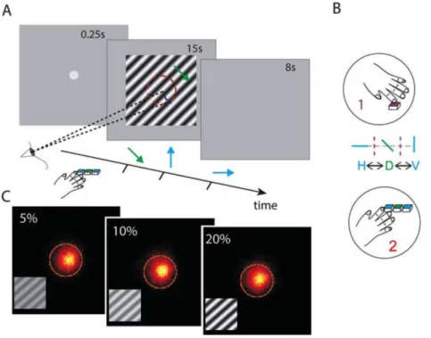
Figure 1: Stimulus and task illustration. (A) Panels showing trial sequence of 0.25s fixation, 15s moving grating stimulation and then a grey screen for 8s. Participants make button presses to indicate each change in perceived direction during stimulation and eye movements are recorded. (B) Button presses reporting transitions were collected either as a single report (task 1) to indicate when perceived direction changed without specifying direction in a simplified task; or with three directions H, D and V explicitly recorded (task
2), reported by participants to be a more difficult task. (C) Three panels showing eye position heat maps with
combined recordings from all observers at three example contrasts of 5, 10 and 20%, inset gratings illustrate the contrasts near both ends of the tested range. Gaze remained largely within the central 3° of visual angle during the task demarcated by the orange circles.
Procedure
Participants sat in front of the screen and kept fixation on a grey spot of 0.27° diameter before each trial. Fixation disappeared and the stimulus appeared for 15s (see Figure 1A) while eye movements were recorded. This duration was a compromise between the need to maximize recorded perceptual switches up against restrictions to minimise effects of observer fatigue, blinking and adaptation of the local motion detectors resulting in motion after effects. The instruction was to respond to indicate the precise instance of each
transition between three perceived direction choices, horizontal (H), diagonal (D) and vertical (V). This response was made in two ways: with a single button press marking the timing of each transition and recording no distinction between actual directions (easier condition: task. 1, Figure 1A-B) or alternatively with one of three button presses at each transition corresponding to H, D or V (reported to be a more difficult condition: task. 2, Figure 1A-B).
Each experimental block was made up of either 36 (task 1) or 42 (task 2) trials, each containing six contrast conditions (c = 0.03, 0.05, 0.08, 0.1, 0.15, 0.2 i.e. 3-20%). There was an 8s wait after each trial before the observer initiated the next trial with a button press. Each block was repeated six to eight times for
task 1 and eight times for task 2, after a couple of initial blocks to familiarise participants with the task. Bad
trials e.g. excessive blinking, containing many abrupt eye movements unlikely to be stimulus driven or self reported ‘bad blocks’ of lapsed attention were discarded. Note that Task 2 has been explored extensively in a separate study, fully characterising the changing patterns in the relative prevalence of each of the perceptual choices (Meso & Masson, 2015). The present study builds on that work with a larger data set and a focus on the analysis of perceptual switching probed dynamically with the additional tool of smooth eye movements. The use of the simplified task (task 1) allowed inexperienced participants to perform the experiments more confidently than task 2. The choice of design omitting useful direction information was made because the complexity added by three separate button presses (H, D or V) made it too difficult for most inexperienced participants whose data we deemed critical for generalising our results.
Perceptual report analysis
We analyse the trend in the reported transition rate as a function of stimulus contrast by fitting the experimentally measured switching rates (both for individual observers and grouped averages) to two nested nonlinear functions which either rise to an asymptotic point of saturation (Equation 3) or rise to a peak (Equation 4) before gently descending with contrast.
𝐹! 𝑐 = 𝐴𝑚𝑝 !!
!!!!"! (3)
𝐹! 𝑐 = 𝐴𝑚𝑝 !!
!!!!"! ×(1 − 𝑐!!) (4)
The basic function is the Naka Rushton used only for its convenient shape, and not intended to imply any underlying contrast response processes at this stage. The terms are the amplitude Amp, the exponent n, the C50 term Cf and for the peak function of Equation 4, there is an additional super saturation exponent term ss. The data is fitted to both these functions using an iterative least squares processes to identify the best parameters. A Kolmogorov-Smirnov Goodness of fit test for significance is carried out on the results of each of the pair of fits and the results are then further compared using the Akaike and Bayesian Information Criterion measures (AIC/BIC). These measures use likelihoods from the fits to determine which model provides a better explanation for the data, taking into account the number of parameters, thus penalising less parsimonious models (Akaike, 1981; Schwarz, 1978; Wagenmakers & Farrell, 2004).
Eye movement recordings and analysis
Eye movements have often been recorded to probe perceptual multi-stability (Hayashi & Tanifuji, 2012; Logothetis & Schall, 1990; Niemann, Ilg, & Hoffmann, 1994; Quaia, Optican, & Cumming, 2016). Barberpole motion stimuli are known to drive reflexive tracking eye movements whose dynamics reflect that of the global motion direction (Barthelemy et al., 2010; Masson et al., 2000). Thus, essential information can be extracted from the temporal dynamics of eye velocity about the instantaneous state of the motion representation and transitions between states. However, such slow eye movements can change the pattern of retinal motion. We included an intermittently re-appearing central fixation spot during the 15s stimulus presentation which observers were instructed to use to initiate a saccade back to the centre of the stimulus. The fixation interval was either randomised between 1.5-3s for each reappearance or fixed at a constant value within this range for different blocks. Controls confirmed that the fixation interval period made no difference to the perceptual switching rate. This interrupted fixation paradigm allowed brief but significant epochs of small tracking eye movements, while maintaining the visual motion input roughly constant over time, as illustrated by the eye positions in Figure 1C. Data to be analysed was collected once participants reported being comfortable with the task and instructions, and blinking and switching rates had settled down accordingly, typically after 1-3 practice blocks.
Right eye movements were recorded with the video eye tracker at a frequency of 1KHz (examples, Figure 2). The eye-position data was first low pass filtered with a Butterworth filter (6th-order, 50Hz).
Velocity traces were derived from the two-point central difference between the symmetric-weight moving averages of the position samples. Standard criteria were used to identify the start and endpoints of both saccades and blinks in these traces (Engbert & Kliegl, 2003), using specific algorithm parameters identical to those detailed in a previous work (Meso, Montagnini, Bell, & Masson, 2016). An extension of an additional 20ms before and 30ms after each of these events were identified for exclusion along with the events to conservatively restrict the traces to just the smooth sections containing gaps, e.g. Figures 2, right hand column. Combination of the x and y velocities was used to obtain the direction θt estimated from the inverse
tangent of the ratio of y and x components. Operations on eye direction were made in a circular space after aligning all stimulus directions (Berens, 2009). Processing described in this section was carried out using bespoke Visual C++ and Matlab routines.
Predicting perceived direction from eye direction
To generalise the relationship between the categorical transitions in perceived motion direction (H-D-V) and the changes in eye direction, we sought to establish whether time averaged eye direction distributions could be used to predict which state (H, D or V) had been reported during each button press in task 2. We designed a three parameter decoding scheme using the time averaged eye direction μθ estimated over a duration
defined by the first decoding parameter, a variable temporal window size N, 𝜇!=!! 𝜃!, 𝑡 ∈ −!!, −!!!! , … , +!! , (5)
and the resulting spread in the form of the standard deviation σθ,
𝜎
!=
! !!! !𝜃
!− 𝜇
! !, 𝑡 ∈ −
! !, −
!!! !, … , +
! !,
(6)N could be in one of three configurations along the eye trace: symmetrically centred around the instance of
the button press equally extending both before and after it (symm., case 1), running from the past before the button press and stopping at the button press (pre-button, case 2) and starting from the button press and stopping some time after in the future (post-button, case 3). The generated mean, μθ and spread, σθ
parameters serve as inputs into a piecewise decision operation which assigns a perceived direction using the second and third parameters, PTH and PTV.
𝐷𝑖𝑟(𝜇
!, 𝜎
!) =
𝑉 ∶ 𝜇
!− 𝑘𝜎
!≥ 𝑃𝑇
!𝐻 ∶ 𝜇
!+ 𝑘𝜎
!≤ 𝑃𝑇
!𝐷 ∶ 𝜇
!− 𝑘𝜎
!< 𝑃𝑇
!𝑎𝑛𝑑 𝜇
!+ 𝑘𝜎
!> 𝑃𝑇
!(7)
In this formulation, the average direction μθ is compared to the two threshold parameters PTH and PTV after
the addition of the spread parameter scaled by a constant k (fixed at k=0.25 following initial optimisation), which captures the fact that it is the distribution rather than just the mean, whose position within the direction space is being categorised. Predictions are then made for a range of combination of values (375,000) of simulated symmetrical, pre-button and post-button temporal windows N, and parameters PTH/V to find the
combination which optimises correct prediction for each of the participants’ individual data sets. To obtain estimates of chance performance for comparison as a baseline, the shuffled set of the recorded perceptual choices made by each participant are re-assigned as decisions for each recorded transition.
Mathematical model overview
Global motion integration is often described as a two-stage process. First, local motion is sensed by a set of spatio-temporal filters with small receptive fields. Here we assumed that a set of different local motion filters extract grating and terminator motion directions (Castet & Wuerger, 1997; Lorenceau, Shiffrar, Wells, & Castet, 1993; Sun, Chubb, & Sperling, 2015) to generate a local motion representation. Information can then be integrated at a subsequent global motion stage where a population of direction-selective cells can encode the 2D motion direction of the whole pattern (C. Pack & Born, 2001; Stoner & Albright, 1996). The dynamics of global motion computation can be seen as the outcome of a diffusion process in both the direction domain and retinotopic space (Tlapale, Dosher, & Lu, 2015; Tlapale, Masson, & Kornprobst, 2010). For the sake of simplicity, we restricted the global stimulus representation to a continuous feature space of direction, a one-dimensional representation. A key feature of this space is that transitions between two perceptual states are dynamic shifts in the dominant peak of the distribution of activity within this population, providing a richer description than discrete jumps between separate states. Mutual inhibition was set between the underlying competing sub-populations of direction-selective cells as a centre-surround interaction kernel. This departs from the typical classical approach where transitions are modelled between two or more discrete neuronal populations, for instance with binocular rivalry (Lehky, 1995; Matsuoka,
1984) or tri-stable plaid patterns (Huguet et al., 2014). While reductions from continuous descriptions to discrete models have been shown to accurately capture the characteristics of dominance duration for binocular rivalry (Laing & Chow, 2002), the richness of representation afforded across continuous perceptual spaces can be exploited in modelling the tri-stable motion direction space (Rankin et al., 2014; Rankin, Tlapale, Veltz, Faugeras, & Kornprobst, 2013).
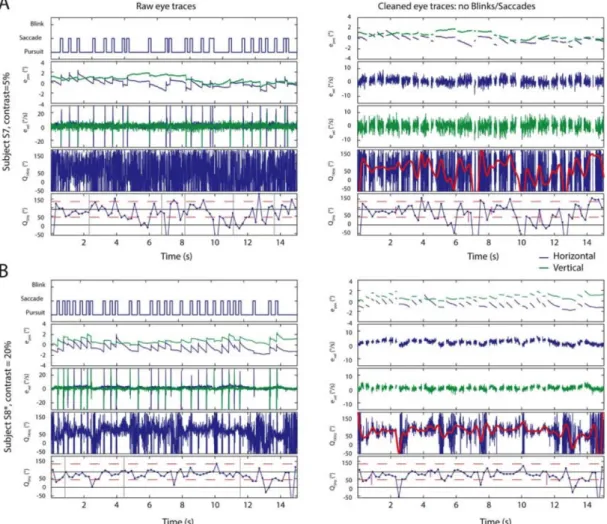
Figure 2: Raw eye movement traces and initial ‘cleaning’. (A) A single trial example of eye movement responses for task 2, participant S7 and contrast 5% over the 15s trial (time on the x-axes of all rows). On the left hand side column, data is in the ‘raw’ form received from the video eye tracker. First row shows validity (i.e. valid, saccade or blink based on standard criteria). Then x (blue) and y (green) position showing abrupt changes during saccades. Third row shows x and y velocities. Fourth, directions at 1000Hz and finally the same direction estimates re-binned at 5Hz for illustration of low frequency content. On the right hand side column, ‘cleaned’ data after applying a conservative removal of blinks and saccades to leave smooth
responses. First a row with the x and y positions with gaps. Then x and y speeds separately with fewer abrupt changes seen than corresponding raw traces. Fourth the high resolution direction trace with gaps is not fully distinguishable from the raw trace. A smoothed trace of the underlying trend is overlaid in red for illustration. Finally the direction trace re-sampled at 5Hz to show more gradual dynamic changes in direction shown alongside the explicit perceptual reports (magenta vertical lines) made by this participant. (B) A second single trial example of raw eye movement responses for participant S8 at contrast 20% over the 15s trials, in the same format as (A). On the left hand side column, the rows shows validity with several saccades, position with the abrupt changes, x and y velocities and directions at 1000Hz and re-sampled at 5Hz. Notably, looking at the last two rows for this participant when compared with (A) demonstrates the observation we made that the variability of participant eye direction produces idiosyncratic patterns which also vary with contrast. On the right hand side column, ‘cleaned’ data is obtained with the same process described above and data is in the same format. Rows are arranged as: positions with gaps, x and y speeds separately, high-resolution direction traces (overlaid with a smoothing function in red) and then the direction trace re-sampled at 5Hz showing more gradual dynamic changes in direction and switching reports (magenta lines).
Using neural fields equations (Amari, 1977; H.R Wilson & Cowan, 1972), a population of direction selective cells such as found in the Middle Temporal cortical area (MT), was modelled as the time varying average membrane potential p(v,t) over the continuous feature space of direction (v). The initial theoretical development is fully described in our previous computational work which details the use of bifurcation analysis to tune the early model, the basic choice of physiologically plausible model parameters for Equations (8) and (9) and the full description of the choices surrounding the model input (Rankin et al., 2014). Here, the most relevant aspects of the model developed in the current work are briefly described. The tri-stable dynamical system includes adaptation α(v,t) and noise X(v,t) terms acting across direction, v as well as a constant input term I(v) which captures the competing direction cues. The main equations describing the dynamics are: 𝜏! 𝑑 𝑑𝑡𝑝 𝑣, 𝑡 = −𝑝 𝑣, 𝑡 + 𝑆 𝜆[𝐽 𝑣 ∗ 𝑝 𝑣, 𝑡 − 𝑘!𝛼 𝑣, 𝑡 + 𝑘!𝑋 𝑣, 𝑡 + 𝑘!𝐼 𝑣 − 𝑇] (8) 𝜏!!"!𝛼 𝑣, 𝑡 = 𝛼 𝑣, 𝑡 + 𝑝(𝑣, 𝑡) (9)
The timescales of Equations (8) and (9) are governed by τp and τα. For Equation (8), the standard decay
term is –p and S is a sigmoidal function with slope parameter λ and threshold T used to constrain the firing rates. The value of λ is analogous to the gain of the contrast response, as estimated using the Naka-Rushton function (Naka & Rushton, 1966). When the maximum contrast response is fixed at 1, one single parameter determines the contrast sensitivity, the half-saturation response contrast (C50). Gain coefficients for the input,
adaptation and noise terms are kI, kα and kX respectively. The noise X(v,t) used is generated by an
Ornstein-Uhlenbeck process selected to allow linear transformation of the space-time variables. Lateral interactions across the direction space are set by a centre-surround interaction kernel J that is defined by three Fourier modes and a Mexican-hat shape where a local excitatory becomes inhibitory for more distant directions.
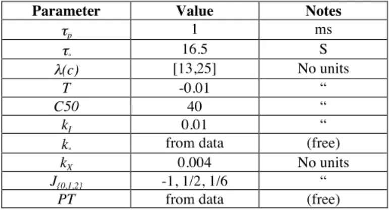
Parameter Value Notes
τp 1 ms τα 16.5 S λ(c) [13,25] No units T -0.01 “ C50 40 “ kI 0.01 “
kα from data (free)
kX 0.004 No units
J{0,1,2} -1, 1/2, 1/6 “
PT from data (free)
Table 1: Parameters for the neural field model of tri-stable motion integration
Values for these parameters (summarised in Table 1) were constrained based on known properties of cortical area MT from human and non human primate neurophysiology, such as direction tuning and inhibitory interaction of units (Qian & Andersen, 1994; Qian, Andersen, & Adelson, 1994; Treue, Hol, & Rauber, 2000), normalization (Carandini & Heeger, 2012) and contrast response functions (Sclar, Maunsell, & Lennie, 1990). A complete description of the extensive parameter exploration and tuning can be found in (Rankin et al., 2014). The principle behind the model construction was to set up a dynamical system that faithfully captures the key properties of visual motion integration. To achieve that aim, it was not necessary for us to have a one to one mapping between neurophysiological structures and each of the model parameters.
Equations (8) and (9) were solved using a standard Ordinary Differential Equation solver in Matlab. We used a numerical continuation package AUTO (Doedel, 1997) to perform Birfurcation analysis to look at the positions of steady state and oscillatory solutions and study the stability of these while a pair of critical stimulus and model parameters (in this case contrast and kα) were varied (Kuznetsov, 1998). AUTO monitors
the stability of states being tracked using this information to detect Bifurcations, the points at which there is a sudden change to a qualitatively different type of solution for a non linear dynamic system as a parameter is changed. Away from bifurcation points this tracking information tells us how the relative stability is
changing with respect to parameters, a measure providing a powerful predictive tool in the current context. For simplicity, this ‘stability’ output can be quantified by the real part of the Eigenvalue for the non-oscillating state which corresponds here to the direction D. We call this output E. In contrast, the real part of the so called Floquet exponent we term F is similarly informative about the oscillatory or H-V (cardinal direction) states (Kuznetsov, 1998). E and F quantify the timescales of growth, or decay of perturbations towards steady and oscillatory states, respectively, so states are stable if these measures are negative and become less stable when the values increase.
The model simulations presented in the current work used a constant input I(v) which is a tri-modal smooth function across the continuous direction space v with a peak centred at the diagonal (v=0) flanked by two peaks on either side (±45 degrees). These peaks were described by Gaussian functions I1D(v) and I2D(v)
with sigma width of 18 degrees for the 1D and 6 degrees for 2D. These 1D and 2D contributions were summed to produce the input function I(v). The weighting in this summation has a contrast dependence built into the 1D term.
𝐼 𝑣 = 𝑤!!𝐼!!(𝑣) + 𝐼!! 𝑣 − 45 + 𝐼!!(𝑣 + 45) (10)
𝑤!! = 0.5 − 0.6𝑐 (11)
The form of Equations (10) and (11) are motivated by previous behavioural experiments on both humans and macaque monkeys demonstrating the changing role of 1D and 2D cues over the time course of visual motion integration (Barthelemy et al., 2010; Barthelemy et al., 2008; Masson et al., 2000). The desired cue relationship captured by this formulation holds for the contrast range over which the current stimulus is seen as tri-stable and continuously moving i.e. below about 40%. Above this contrast, adverse motion after effects influencing the perceived speed emerge and in Equation (11) w1D is therefore set to zero above c=5/6.
This limit marks the edge of the parameter region beyond which multistability can no longer be perceived or indeed modelled. The resulting effect of contrast on input signal to noise ratio which determines the dynamic weighting of these competing cues is consistent with previous work (Lorenceau & Shiffrar, 1992).
Zero noise case: Bifurcation analysis
Bifurcation analysis is run with the noise coefficient kX set to zero and used to identify parameter regions that
conform to expectations following initial psychophysics experiments. The aim is to restrict the range of values of the adaptation gain (kα) so that the model can best account for the non-monotonic relationship
between perceptual switching rate and contrast. With strong adaptation (kα=0.03) the onset of switching at a
critical value of the contrast is sharp, the falling phase of the switching rate is captured in this case but not the rising phase. With no adaptation (kα=0) the switching rate would increase monotonically. The tuning
process seeks to identify an intermediate range of values of adaptation strength (later set near kα≈0.01) at
which the experimentally observed rising and falling phases of the switching rate curve are both possible.
Added noise: dynamic direction simulations
Simulations are subsequently run with a non-zero noise coefficient (kX =0.004). The goal is to generate a
continuous dynamic direction output of high temporal resolution modelling the cortical global motion representation during the competition in each trial. This can be read out in various ways and compared both to the continuous eye traces and the perceptual decisions under the range of contrast conditions. The main readout subsequently reported is a count of the number simulated percept changes between direction states, H, D or V over each of the 1500 simulated trials (used as our standard number of simulated trials) carried out per contrast value over the tested range. To count switches, a pair of threshold values are applied to the dynamic peak of p(v,t) set at a distance ±PT from the diagonal. PT captures the fact that given a forced choice decision along a continuous space, participants will make a categorical forced choice decision based on boundary criteria which will vary across individuals (see also Equations 5-7; PT ∝ PTV-PTH); this
parameter sets this boundary between H, D and V in direction space. The model implementation assumes symmetry between H and V in the direction space though we note that the actual data shows biases across this space. It is our first critical free parameter when bringing the model into an operating regime in which it can be tied to individual participants. The second free parameter is the adaptation strength kα. Low-level
visual adaptation dynamics show some variation across individuals that is captured by this parameter. In the perceptual competition between directions, small shifts in its value impact the transition rates, allowing us to adjust the simulated rates according to individual performance. Finally, the normalised direction distributions
of the full dynamic model output p(v,t) generated for the simulations over the range of contrasts give the predicted percept probability across the direction space. This can be compared directly to the eye direction distributions over corresponding contrast ranges. We test for changes in these distributions by fitting multimodal nested functions FD, of 1-3 peaks modelled by Lorentzian functions (typically sharper than
Gaussians, providing a better fit to the current data) to quantify whether the modality of these distributions (i.e. one dominant peak or multiple peaks in eye direction) changed across the tested contrast range. The general form of the fitted function is,
𝐹! 𝑣 =
𝐶 +
𝐴𝑚𝑝𝑛×𝑆𝑖𝑔𝑛2 𝑆𝑖𝑔𝑛2+(𝜃−𝑃𝑒𝑎𝑘𝑛)2𝑖
, 𝑖 ∈ {1, … , 𝑛} , 𝑛 ∈ {1, 2, 3}
(12)Eye direction distribution data binned into 180 bins of 2° each are fitted to Equation 12 using a nonlinear least squares fitting to find the best parameters for three versions of the function with one mode (n=1), two modes (n = [1,2] ) and three modes (n = [1,2,3]). The fits therefore have four, seven and ten parameters respectively, so the comparison between them is done by AIC and BIC to find which function best describes the number of peaks in the distributions. This is done both for individual data distributions and those from the grouped data.
Results
Dynamic coupling between reported perceived direction and eye direction
Previous work has demonstrated a link between perception and smooth eye movements during ambiguous perception of binocular rivalry stimuli (Hayashi & Tanifuji, 2012). We tested a similar premise in the current work, analysing the smooth portions of eye movement traces during presentation of an ambiguous barberpole stimulus. We focused on the smooth phases of eye movements, which are driven by the motion stimulus. Therefore blinks and saccades causing abrupt changes in eye direction and speeds were identified and excluded from the analysis (e.g. typical individual trials Figures 2). Eye direction was estimated from the inverse tangent of the ratio of the speeds in the x- and y-directions and this nonlinear estimate is therefore highly susceptible to noise (see fourth row, left hand column in Figures 2). Once traces were cleared of the most abrupt changes in eye position and speed, smoother traces appeared with gaps (see right hand column of Figure 2). Underlying dynamic trends in eye direction can be seen in the noisy traces in the fourth row of this right hand column of Figure 2, in the thick red lines which are the result of applying a generic smoothing, for illustration only. A similar trend can also be seen in the same data sampled at 5Hz in the last rows of panels in Figure 2, where instances of button presses are also included. These example results highlight the noisy nature of the individual traces obtained, the need for appropriate filtering (which is fully detailed in the methods section) and the inherent limitations in trying to determine instantaneous motion direction perception from this dataset without prior knowledge of the instance of button presses.
In an initial exploration of the relationship between eye direction and perceptual decisions, data from
task 2 (in which participants explicitly reported eye direction) was studied. Dynamic eye direction traces
were considered by plotting the averaged traces obtained combining across participants, restricted to ±0.75s around each button press for the different reports (H-D-V), separated by contrast (Figure 3A-C). The resulting averaged traces show that when eye direction is aligned with the button press (thick vertical black line), the reported direction is related to the eye direction for all tested contrasts. By looking at this data, it is clear that there is an optimal time window within the dynamic trace (illustrated inset, Figure 3C) over which the eye direction is most indicative of the perceptual decision. It can also be seen that averaged eye traces are largely separated across the direction space so that beyond a threshold [e.g. PTV in Figure 3B] up from the
diagonal, traces will typically correspond to a perception of V. To interrogate the spread within this data, the averaged eye direction traces extending through the same range (±0.75s around each button press) are then binned into histograms (50-bin width) separated by decision (H-D-V) and contrast condition. The resulting distributions are shown in Figure 3D-I. The direction densities for the cardinal directions H and V are consistently seen to flank the D density in green on either side. The differences between the means and modes (inset in the figures, black and grey lines respectively) of the H and V distributions quantify how separated the peaks are and therefore show an approximate increase in separation as contrast is increased. These distributions demonstrate intuitively how the effectiveness of a decoding process depends on the distributions within the direction space, hence relate to the PTV and PTH parameters. They also show that we
might expect different optimal values across the contrast range.
To determine the optimum eye direction window parameters across our dataset, we use the insights gained by visualising the data as described above to devise a simple three parameters decoding scheme (see Equations 5-7 and methods). The scheme computes a forced choice decision (H-D-V) for each trace based on
the window length N (in ms) of the eye direction trace and the pair of threshold parameters PTH/V. When this
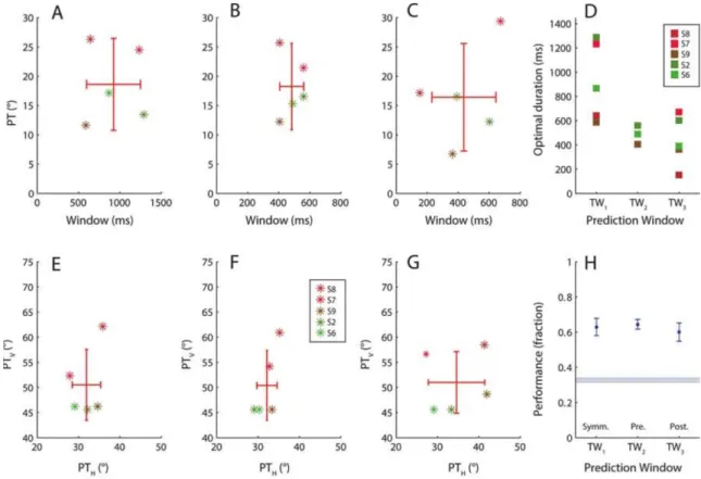
decoding scheme is applied to the data for each of the participants who did task 2, the optimum prediction results can be compared for the symmetrical window of eye directions extending equally before and after the button press (Figure 4A), the pre-button window (Figure 4B) and the post-button window (Figure 4C). The top row shows the optimally fitted PT values for each participant (∝ PTV-PTH) plotted against temporal
window size. The parameter distribution showing the least spread when the different window configurations are compared corresponds to the pre-button window (see Figure 4D), which notably uses approximately half the eye direction information than the longer symmetric window for the decision.
For this pre-button window, the optimal duration values are seen to be distributed between 400-500ms across participants and PTV/PTH show a range of values which all reveal the asymmetry in the direction space
for the empirical data (H-bias, see also Figures 3D-I). The complete results for optimal fitting and subsequent decoding including a comparison of the three window configurations are given by Table 2 and Figure 4H. These include the baseline performance of around 36% shown with standard deviation in horizontal blue lines of Figure 4H obtained by shuffling the response data and using them to re-assign randomised decisions. The average prediction performance of the selected pre-button window is 65% and therefore almost 30% higher than the baseline, a performance slightly higher than the alternative window configurations. We note that we were indeed able to achieve even higher prediction performance (>80%) by optimising separate classification parameters for each contrast. The resulting parameters from those simulations would be less general and such extensions are therefore beyond the aim and scope of the current work. The present results reliably indicate that changes in time averaged eye direction precede the button press by several hundred milliseconds reflecting the button press choice and therefore help elucidate the constrained window in which these two measures are most related. This window is about 484±77 ms before the button press. We acknowledge that in this decoding result, we were unable to achieve the more difficult goal of reliably determining when within an eye movement trace a perceptual transition occurred. Though further work towards that goal continues, this may well also be limited by the variability of individual eye movement traces. We instead rely critically on the complementary nature of our two behavioural measures.
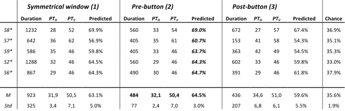
Symmetrical window (1) Pre-button (2) Post-button (3) Duration PTH PTV Predicted Duration PTH PTV Predicted Duration PTH PTV Predicted Chance
S8* 1232 28 52 69.9% 560 33 54 69.0% 672 27 57 67.4% 36.9% S7* 642 36 62 56.9% 405 35 61 60.7% 153 41 58 54.3% 35.1% S9* 586 35 46 59.8% 405 33 46 63.7% 363 42 49 54.5% 35.3% S2* 1288 32 46 64.5% 560 29 46 64.3% 602 33 46 59.8% 33.0% S6* 867 29 46 64.3% 490 30 46 64.7% 391 29 46 61.8% 37.9% M 923 31,9 50,5 63.1% 484 32,1 50,4 64.5% 436 34,6 51,0 59.6% 35.6% Std 325 3,4 7,1 5.0% 77 2,4 7,0 3.0% 207 6,8 6,1 5.5% 1.9%
Table 2: Best fitting parameters from the application of the prediction scheme described by Equations 5-7. Predictions are divided into the three window types and shown separately for the five participants who did
task 2. Based on this data, 2 is chosen as the best window of prediction. The effect of grating contrast on reported perceptual switching rates
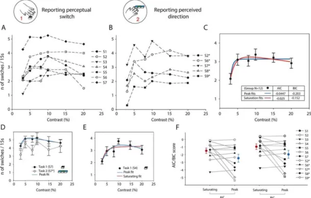
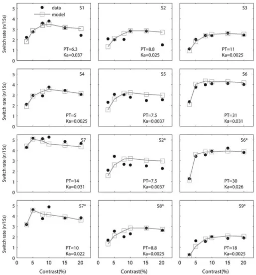
Varying the contrast of the grating is one way of modulating the strength of the stimulus. For each value within the range of contrasts tested (3, 5, 8, 10, 15 and 20%), we plotted the average number of transitions reported per 15s trial for each one of the participants who performed the task. These are shown for both task
1 and task 2 in Figures 5A and 5B respectively. The increase in reported transitions as contrast rises from 3%
can be seen for almost all participants and, in some of them a gentle reduction at higher contrasts can also be seen. The results from the two tasks are similar, though task 2 was more difficult and thus showed more variability in the trends. We ask whether these plots are better fitted by a rising and saturating function or whether the gentle reduction in switching rates at higher contrasts is indeed significant. We do this by fitting all the data for the two tasks combined with either a saturating function in Equation 3, or the same function with a supersaturating term added to make it a peak function, given in Equation 4. The resulting fits are shown in Figure 5C, with the actual data shown by the points and standard error bars overlaid with the saturating (blue line) and peak (red line) function fits. We apply the model comparison BIC and AIC tests
described in the methods section on the pair of fits and find that with both measures, the peak function has a lower score for both AIC (-0.045 vs -0.025) and BIC (-0.2 vs -0.15) indicating that it is indeed a better overall description of the trends observed. This trend was obtained for the whole data set and we ask the same question for the 12 individual participant’s data which show some variation even between task 1 and
task 2 (e.g. Figure 5D), and which can also be fitted by peak and saturating functions individually (e.g.
Figure 6E). We repeat the procedure, obtaining fits for both function types and then calculating the AIC and BIC comparison results for individual fits (see Figure 5F). Most traces show a lower score for the peak than saturating functions and when we consider the individual scores and directly compare them for the pair of functions, we find a significantly lower value for the peak scores in a one tailed t-test for both the AIC (means -2.48 and -1.50; t(11) = -1.99, p = 0.036) and BIC (means -2.65 and -1.64; t(11) = -2.05, p = 0.032). Therefore our results demonstrate (both at group and individual levels of analysis) that the switching rate rises fast at low contrasts, peaks at mid contrasts around 8-10% and then decreases gently – though at different rates for different participants.
Dynamic Neural Field Model construction and simulations
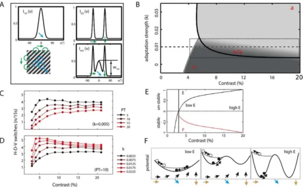
We now seek to extend and adapt our previously proposed model of tri-stable motion perception (Rankin et al., 2014) to the experimental observations to enable us to run simulations with perceptual switches. The cardinal and diagonal inputs, with respect to the competing directional cues within the input grating stimulus, are defined as Gaussian functions of 6° and 18° widths respectively (Figure 6A). We first used bifurcation analysis (Kuznetsov, 1998) to study the relationship between the dynamical behaviour of the underlying tri-stable neural system and two parameters: the adaptation strength (kα) and the contrast (c). The model
represents the continuous perceived direction space with the dynamic function p(v,t) which peaks at just one ‘winning’ direction following the application of mutual inhibition across direction space, resulting in a peak which drifts across the direction space over time. The purpose of bifurcation analysis was to identify qualitatively different regions of interest in this parameter space and work within regions with dynamic properties comparable to the experimental data. The bifurcation curves plotted in Figure 6B were computed without noise (kx = 0). The curves bound three parameter regions with different dynamics: in white, a low
contrast regime where the system is below threshold (the input is not detected); in light grey, regular oscillations (switches) are driven by adaptation, and in dark grey, no switching is predicted in the deterministic (no noise) case. When noise is added (kx ≠ 0), switching in the light grey region of Figure 6B
remains driven by adaptation and is therefore labelled a. In the dark grey region of the same figure with zero or very low adaptation strength, switches can only be driven by noise so we label this region n. In a parameter tuning explained in the Methods section, we identify an operating regime for the model where the switching rate relationship found in the experiments (Figure 5) is best accounted for. This zone lies near the transition between the regions n and a (thick black curve in Figure 6B, within the dotted rectangle labelled n/a). Within this rectangle, there is a shift in the dominant mechanisms driving the switching behaviour from noise to adaptation as contrast is increased, shown by the gradation of shading from dark to light grey.
Within the parameter region which generates the required model behaviour, we select two free parameters for the simulations – the adaptation strength kα and the perceptual threshold PT which fine tune
the switching rate functions to allow them to vary with the range of trends observed in the experiments (Figure 5A-B). PT demarcates the direction space separating what is considered D, from H and V. It defines the symmetrical distance from the diagonal at D=45°: when the value of the peak of the dynamic function p(v,t) falls below 45-PT, direction is H (i.e. PTH in the eye movements), and above 45+PT, the direction is V
(i.e. PTV in the eye movements). We assume symmetry in the model even though this is not the case in the
eye traces, where an H-bias can be seen. The effect this parameter has on simulated switching rates is shown in Figure 6C, where it is seen to shift the function up or down and change the steepness of the low contrast rise. The kα parameter determines the strength of adaptation controlling its depth of modulation across the
direction space. When it is finely controlled, restricting it to within the rectangle identified in the bifurcation analysis, this parameter is seen to shift the position of the switching rate peak and the extent to which there is a reduction in switching rate at higher contrasts (See Figure 6D). Finally, the stability parameters obtained during the bifurcation analysis and described in the methods section, the Floquet exponent, F (red trace), corresponding to the adaptation driven transitions and the Eigenvalue of the steady solution corresponding to the noise driven transitions, E (black trace), are plotted for the contrast range in Figure 6E. The change in stability predicted with increasing contrast can be visualised through potential wells within which gravity acts on a particle, illustrated in Figure 6F. Dominance in the D directions shifts systematically towards the cardinal directions as stimulus contrast is increased.
Using model simulations, we find the best fitting parameters (PT and kα) for each of the 12 data sets so
that we can compare the empirical and simulated switching rate functions by plotting them together (see Figure 7, compare simulated grey squares with data in black circles). We find that through variation in the two parameters, the model is able to closely capture the full range of trends reported by the participants across both tasks. Note that the range of fitted PT values in the simulations is as broad as that seen in the eye movement data of task 2, in Figure 4A-C.
Further testing of model predictions
Using the best-fitted PT and kα parameters for all the data combined (PT=13.125, kα =0.01125), simulations
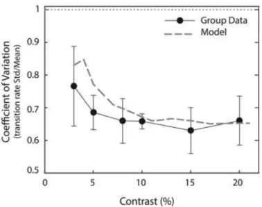
are then run across the contrast range to extract additional statistical properties of the perceptual switching. The first of these is the coefficient of variation (CV) of the time between switches for each contrast, which is calculated as the variance of percept durations divided by the average of percept durations. The results are shown in Figure 8. The model predicts a gradual reduction in CV (grey dashed trace) from 0.85 as contrast is increased from 3 to about 10% before the value plateaus at around 0.65, which is maintained for the rest of the contrast range. A similar trend is observed for the experimental data (black circles) with the standard error of CV across participants given by the error bars. This trend is driven by a shift from highly variable percept durations for the low contrast noise driven transitions, towards slightly less variable durations during the adaptation dominated transitions at higher contrasts. The model predicts a slightly higher variability than the experiments in the low contrast range where noise dominates, but model and data converge at the mid and higher contrasts.
The consequences of the shift in stability predicted in Figures 6E-F as contrast is increased were tested. The rationale is that the most stable parts of the continuous direction space illustrated as the bottoms of potential wells would act as attractors in the system and as a result peaks would occur in the dynamic representation of perceived direction. This is first shown with the simulations in Figure 9A, where a distribution of the dynamic value of the peak of p(v,t) obtained from 1500 simulations of 15s each are plotted for three contrasts: 3, 8 and 15%. It can be seen in this prediction that there is a clear transition from a uni-modal distribution centred on the diagonal direction (black dashed trace) towards biuni-modal distributions which increase in separation as contrast is increased (grey dashed lines). To test this prediction with the experimental data, we use eye movements recorded from task 2 and separate out eye directions obtained for H, D and V button presses restricted a critical 450ms time window before the button press and plot the peak direction (and inter quartile range as error bars) for the contrast range tested (see Figure 9B). What we see is a progressive increase in the separation of peaks as contrast is increased, consistent with the predicted increase in stability, the same trend as the simulations but asymmetrically skewed towards the H direction in the empirical data. The use of the peak of the p(v,t) function was necessary because when the full continuous function is considered unrestricted to the 450ms ‘decision window’, the resulting distribution is broader and does not clearly show the separate underlying peaks (see Figure 9C, obtained for the same simulations as 9A). Because eye direction in the current experiment was a continuous empirical measure, these simulated distributions were analogous to those produced when all the eye direction data from both tasks were plotted combining all the H-D-V button presses indiscriminately, in Figure 9D. The eye data distributions no longer show clearly discernible peaks, but get progressively wider with increasing contrast.
The last challenge was to quantify the shift in these distributions of eye directions with no clearly discernable peaks (see individual examples in Figures 10A). This is done by fitting the distributions with a Lorenztian function in Equation (12) which can have one, two or three superimposed peaks (see methods for details). We compare the modality of the group fits in Figure 10B using AIC and BIC tests, which give a lower score for the better model of the distribution. The AIC scores favour the one-peak fit (Figure 10C) at lower contrasts but shift towards the 2 and 3 peak fits (3-peak shown in Figure 10D) at higher contrast, seen in the AIC scores at 3, 8 and 20% contrasts which are -6.74, -5.64 and -5.33 for one peak and -6.10, -6.17
and -7.73 for the three peak function. Very similar numbers are seen for the BIC test, confirming that low
contrasts (<8%) are better modelled as unimodal distributions dominated by the D direction and higher contrasts (>10%) tend towards a multimodal distribution with dominant cardinals but consistently present diagonal directions.
We ran the same test on individual participant data to confirm that the trend is consistent across individual participants, and not driven entirely by single individuals. The participant eye direction distributions are much noisier that the grouped distributions (compared Figures in 10A with 10B) and so some data cases across the six contrast range could not be reliably fitted by Equation 12. For this reason, participant data from S1, S3 and S2* were excluded from the individual data Table 3. The table shows AIC
and BIC values for each participant, separated across different rows for one, two and three mode fits for the six contrasts along the columns. The best fit from each group of three is highlighted in grey (light for uni-modal and dark for multi-uni-modal fits). At the bottom of the data tables, the count of the cases under each modality for low (3 & 5%), mid (8 & 10%) and high (15 and 20%) contrasts cases are shown. These counts show a general shift from unimodal, towards multimodal (both bimodal and trimodal) distributions systematically as contrast is increased. The individual data supports the conclusions from the group data that contrast drives a shift towards multistability, with both bi-modal and trimodal distributions increasing with contrast.
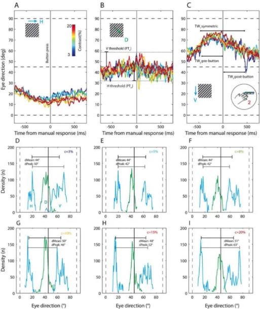
Figure 3: Dynamic averaged eye direction traces and distributions from task 2 restricted to ±750ms from
each button press: (A) Six traces averaged across all participants and colour coded for the range of contrast
(see colour bar inset) for the cases where H-direction was selected, with eye direction (°) on the y-axis and time in ms on the x-axis. The vertical black line at t=0 is the button press. We see that there is a maximum downward deviation from the stimulus diagonal (45°) at the button press. (B) Cases where D was selected in the same format as H above. The traces lie near the dashed line, more below than above it, indicating a slight H-bias consistently seen in our recorded eye directions. The horizontal and vertical thresholds are indicated: these are proposed as a constraint for a scheme predicting perception from eye direction. (C) Cases where V was selected, in the same format as the two above. Traces show maximum upward deviation from the diagonal direction at t=0 for all traces. Inset, three temporal windows of consideration spanning symmetrically before and after [1], only before [2] and only after [3] the button press are illustrated as additional constraints for predicting perception from eye direction. (D) These are also plotted as distributions across 50 histogram bins in the direction space. The density traces for cases where reported directions were in the cardinal direction i.e. button presses H and V, are in blue while the diagonal is in green. The separation between the means and the peaks of the distributions are shown above each trace. For the lowest contrast of 3%, a broad diagonal peak overlapping with the vertical is seen which has the lowest distance between the means of H and V distributions. (E) Distributions for 5% contrast. (F) Distributions for 8% contrast. (G) Distributions for 10% contrast, where the H and D peaks appear to be sharper and further apart. (I) Distributions for 15% contrast, similar to those for 10% contrast. (J) Distributions for 20% contrast, the highest contrast. The peaks of the cardinal components are prominent and furthest away from each other for this contrast. This data is indicative of a systematic underlying relationship between eye direction and perception, though it cannot be characterised fully here as these distributions are based on averaged traces (1500 samples) around the button presses H, D or V.
Figure 4: Optimal prediction parameters linking perceived direction to eye direction in task 2 and prediction
performance. (A) The Perceptual Threshold (PT) obtained by combining the best PTH and PTV is plotted
against window duration, first for the symmetrical window for the five participants. The optimal window distribution on the x-axis is broad for this case. (B) Similar to A, PT against window duration for the pre-button window. The spread along both axes is narrowest for this case. (C) The post-pre-button case shows the largest distribution of optimal PT parameters. (D) Re-plotting all three cases to compare the optimal durations shows that for the pre-button window (TW2) optimal windows seem to fall consistently between
400-500ms. (E) PTV against PTH first for the symmetrical window then, (F) the pre-button window and (G)
the post button window. Most cases have best fitted thresholds biased towards the horizontal direction, considering 45° as the diagonal. (H) The fraction of correct predictions of button presses for all participants based on their individual optimal parameters is plotted for each of the three prediction window types. The baseline chance performance based on choice shuffling is shown in the horizontal blue lines which show the mean and standard deviation across participants. The pre-window in the centre of the plot returns the best performance.
Figure 5: Transition rates from perceptual reports plotted against contrast. (A) Average number of reported transitions per trial for the 7 participants performing the simplified task (1) plotted with different markers showing the variation in individual patterns of perceptual transitions. (B) For the more difficult task (2), average reported transitions per trial for the 5 participants, three of whom also performed the simplified task, are plotted with different markers showing trends generally similar to (A). (C) The data from (A) and (B) are combined and fitted with a saturating (blue line) and a peak (red line) function for comparison. Both functions fit the data. A model comparison using both the Akaike and Bayesian Information criteria (numbers inset) find that the peak function provides a better fit to the data even when corrected for the extra parameter. Scores are shown inset: more negative scores indicating a better model. (D) Examples of data for the two tasks for the same participant S7, task 1 (black circles) and task 2 (white circles). The solid black line shows the best fitting peak function for task 1. (E) Perceptual reports for participant S4 doing task 1, showing both the peak (black line) and saturating (grey line) fits. (F) A comparison of the AIC (left pair of points) and BIC (right pair) scores for individual participants’ switching rate curves. The peak function value is compared to the saturating function and points include data from the 9 participants and 12 sessions. The larger points show the mean and standard error of the scores, returning with better performance for the peak function.