Global sensitivity analysis in welding simulations -- what are the material data you really need ?

HAL Id: hal-00419162

https://hal.archives-ouvertes.fr/hal-00419162

Submitted on 25 Sep 2009

HAL is a multi-disciplinary open access

archive for the deposit and dissemination of

sci-entific research documents, whether they are

pub-lished or not. The documents may come from

teaching and research institutions in France or

abroad, or from public or private research centers.

L’archive ouverte pluridisciplinaire HAL, est

destinée au dépôt et à la diffusion de documents

scientifiques de niveau recherche, publiés ou non,

émanant des établissements d’enseignement et de

recherche français ou étrangers, des laboratoires

publics ou privés.

Global sensitivity analysis in welding simulations – what

are the material data you really need ?

Olivier Asserin, Alexandre Loredo, Matthieu Petelet, Bertrand Iooss

To cite this version:

Olivier Asserin, Alexandre Loredo, Matthieu Petelet, Bertrand Iooss. Global sensitivity analysis in

welding simulations – what are the material data you really need ?. Finite Elements in Analysis and

Design, Elsevier, 2011, 47 (9), pp.1004-1016. �10.1016/j.finel.2011.03.016�. �hal-00419162�

Global sensitivity analysis in welding simulations — what are the material

data you really need ?

Olivier ASSERINa_{, Alexandre LOREDO}b,∗_{, Matthieu PETELET}a,b,1_{, Bertrand IOOSS}c a

CEA, DEN, DM2S, SEMT, LTA, F-91191, Gif-sur-Yvette, France b

LRMA, EA 1859, Universit´e de Bourgogne, France

c_{CEA, DEN, DER, SESI, LCFR, F-13108, Saint-Paul-lez-Durance, France}

Abstract

In this paper, the Sensitivity Analysis methodology is applied to numerical welding simulation in order to rank the importance of input variables on the outputs of the code like distorsions or residual stresses. The numerical welding simulation uses the Finite Element Method, with a thermal computation followed by a mechanical one. Classically, a Local Sensitivity Analysis is performed, hence the validity of the results is limited to the neighborhood of a nominal point, and cross effects cannot be detected.

This study implements a Global Sensitivity Analysis which allows to screen the whole material space of the steel family mechanical properties. A set of inputs of the mechanical model —material properties that are temperature-dependent— is generated with the help of Latin Hypercube Sampling. The same welding simulation is performed with each sampling element as input data. Then, output statistical processing allows us to classify the relative input influences by means of different sensitivity indices estimates.

Two different welding configurations are studied. Considering their major differences, they give a different ranking of inputs, but both of them show that only a few parameters are responsible of the variability of the outputs. To prove it a posteriori for the first configuration, two series of computations are performed for a complete sample and for its reduced copy —where all the secondary parameters are set to mean values. They match perfectly, showing a substantial economy can be done by giving to the rest of the inputs mean values.

Sensitivity analysis has then provided answers to what we consider one of the probable frequently asked questions regarding welding simulation: for a given welding configuration, which properties must be mea-sured with a good accuracy and which ones can be simply extrapolated or taken from a similar material? That leads us to propose a comprehensive methodology for welding simulations including four sequential steps: a problem characterization, a sensitivity analysis, an experimental campaign, simulations.

Key words: Sensitivity Analysis, material properties, random sampling, Finite Element, numerical

experiments, welding simulation

1. Introduction

Control of mechanical effects of welding is a very difficult problem a lot of manufacturers have to solve, especially in the transport and the nuclear fields.

∗_{Corresponding author}

Email addresses: olivier.asserin@cea.fr (Olivier ASSERIN), alexandre.loredo@u-bourgogne.fr (Alexandre LOREDO), bertrand.iooss@cea.fr (Bertrand IOOSS)

1

This work is part of a PhD thesis cofinanced by CEA (the French atomic energy agency) and the Burgundy French region

The Finite Element Method has been proved to be an effective tool for the welding simulation. The high increase in computer power allows nowadays simulating a complex welded assembly with a per-sonal computer, in order to predict, from the con-ception stage, if mechanical behaviour is accept-able.

On the other hand, increasing processes com-plexity demands more and more accurate adjust-ing. Numerical simulation, provided that it can be sufficiently precise, is expected to become an impor-tant tool because it can considerably reduce the cost

of developments. For example, it allows optimiz-ing parameters for special processes as for example in [1], more, it allows investigating new processes without any experimental device [2].

Hence, numerical simulation has to fulfil more and more requirements: control of mechanical weld-ing effects like residual stresses and distortions, sup-port to develop new processes, nuclear safety anal-ysis reports, etc.

However, running a welding simulation requires inputs like mesh geometry, boundary and initial conditions, material properties and process parame-ters. The simulation generates several outputs, in-cluding spatial distributions of displacements and residual stresses in the seam. Among the aforemen-tioned inputs, material properties are numerous.

This leads to one of the key problems of welding simulation. During a welding process, as tempera-ture varies in a large amount, material properties vary strongly. Hence, they need to be inputted as arrays of 5 to 10 values for various temperatures instead of a single value. The number of input ma-terial parameters can rapidly reach high values, typ-ically 50 to 100.

It is quite difficult to use material data published in technical literature: firstly, it is sometimes dif-ficult to find data for a given material apart from the classical ones; secondly, they are rarely charac-terized over a sufficiently wide temperature range. At high temperature, near the solidus temperature, most of these parameters are impossible to mea-sure. More, some mechanical models involve pa-rameters which are not present in classical data banks. On the other hand, for one given material, the full characterization is very expensive, often dif-ficult or even sometimes impossible. For instance, it can take years to characterize a specific mate-rial without anyway knowing if all these data are significant.

To avoid this problem, numerical simulations are commonly done using available material data com-plemented with extrapolated values at high tem-perature and/or data given for a supposed similar material. This is not necessarily a bad method, be-cause it will be shown in the present paper that, for a given problem family, some material proper-ties are not very significant. The problem is to know what is permitted, in other words, the resulting in-accuracy induced by these practices.

Sensitivity analysis (SA) of these numerical mod-els gives a rigorous answer to this question: it per-mits to notify what material properties need to be

precisely determined and on the other hand, if it is possible to use a “mean value” or a “probable value” for some other properties.

Several studies regarding the influence of ma-terial properties in welding simulation are avail-able [3, 4, 5, 6, 7, 8, 9, 10], but none of them can be considered as SA. Indeed, these parameters studies are only based on the comparison of results in terms of stresses and/or displacements of simulations con-sidering different kinds of material properties evolu-tions with temperature. These authors have stud-ied the influence of the thermo-mechanical material properties for various welding cases, with different material and models of material behaviour. Sev-eral papers seems to show that the distortions are mostly affected by thermal expansion and Young’s modulus.

A study in which design variables are optimized to obtain minimum welding residual stresses can be found in [11]. Let us mention [12, 13] whose results tend to show that for the studied cases the distortions are mostly affected by thermal expan-sion and, to a lesser extent, by Young’s modulus and yield strength. Schwenk [13] adds that Pois-son’s Ratio and the strain hardening have no no-ticeable influence on the calculated distortions and they can therefore be described by a master curve corresponding to the general alloy group. More-over, this study shows that Young’s modulus and the yield strength at high temperature don’t have to be measured and can be taken from literature.

Sensitivity Analysis is also useful to solve inverse problem as in design optimisation. A very detailed review of Design Sensitivity Analysis methods can be found in [14] and a lot of later SA works cover-ing various applications includcover-ing weldcover-ing can be found. Many of these approaches need to solve the adjoint problem, or involve partial derivatives which may be computed numerically by varying each input variable within a small interval around a nominal value and determining the corresponding effect on the output variable. However, few of these works deals with welding modelling and influence of material properties is not explicitly studied.

In welding simulations, the works cited above are based on local SA, which is of limited use for several reasons: (i) the validity of the results is limited to the neighbourhood of the studied material(s); (ii) in consequence the results of a local SA in weld-ing simulation don’t provide for an exploration of the rest of the material space of the input factors, i.e. it is improper, on the basis of a local SA, to

make general recommendations on which material properties are necessary to know to perform an ac-curate simulation; (iii) local SA is justified to assess the relative importance of input factors only if the output behaviour is proved to be linear.

Global SA, on the opposite, avoids these prob-lems. In the two last decades, the work of searchers like Morris [15], Helton [16], Saltelli [17], Kleij-nen [18], Iooss [19] helped to promote the use of global SA. Practical aspects of global SA and its ap-plications can be found in the following books [20, 21, 22, 23]. This methodology takes into account the entire variation range of all inputs, and tries to apportion the output variation between them. This technique has been successfully used in a large va-riety of domains.

In this work, complete methodology of the global SA is successfully applied to welding simulation. The input space concerns only the mechanical prop-erties and is extended to all steel materials. This leads to a quantitative classification of the most im-portant parameters. To use this technique, it was necessary to develop specific sample techniques and choose a relatively light problem with the aim to perform a lot of simulations within a reasonable time.

The present paper is organized as follows. In Sec-tion 2, the mathematical modelling of mechanical effects of welding is discussed, firstly with the ther-mal model and secondly with the elasto-viscoplastic mechanical model. In Section 3, we describe the global sensitivity analysis by computations of cor-relation coefficients between input and output vari-ables and we propose a technique for generating Latin Hypercubes samples with a monotonic de-pendence. Samplings and statistical analysis were realized with the SSURFER toolbox [24] developed within the R Software [25]. In the last part of this work, the global SA is performed on two different welding studies.

2. Finite element model

The welding thermo-mechanical problem is solved by the Finite Element Method. In weld-ing problems, the thermal history has a notable in-fluence on the mechanic behaviour because firstly, temperature is directly responsible to the thermal expansion which gives strains and then stresses, and secondly temperature affects mechanical properties like Young’s modulus or the yield strength. On the other hand, the reverse effect is negligible: the heat

produced by mechanical nonlinearities like plastic-ity is very low compared to the one delivered by the welding source. This kind of problem is said to be weakly coupled.

According to this fact, people generally simu-late welding within two times: first the thermal field time evolution is computed solving the time-dependent heat conduction equation; secondly, the mechanical equilibrium equations are solved for each time step, the thermal field, which had been previously computed for this time, token as a ther-mal load. For the mechanical problem, time is not explicitly present (there is no dynamical effects) but the elasto-visco-plastic behaviour creates an evolu-tion which must be stored and updated during the nonlinear solving iterations. Outputs of the me-chanical problem are classically the displacement, strain and stress field histories. For practical needs, displacements and stresses of the last time step, when the process is supposed to be finished, are of particular interest.

2.1. Thermal computation

As mentioned before, the thermal field history is computed solving the time-dependent heat conduc-tion equaconduc-tion. Heat conducconduc-tion is assumed to obey to Fourier’s law, with a temperature-dependent heat conductivity.

The complex phenomena of heat deposit occuring during welding operation, including phase changes, magnetic effects and fluid dynamics are not mod-elled here. The thermal deposit is modelled by means of a parametric volumetric function. This approach is classically considered to be sufficient to deal with mechanical effects of welding. Once the function is chosen, values of its parameters can be calibrated for example by inverse methods based on experiments.

Heat losses are classically convection and radia-tion losses. They are generally relatively low com-pared to the heat provided by the source.

So, the problem to be solved is:

ρ CpT˙− ∇ · (λ ∇T ) − Q(t) = 0 in Ω (1)

where ρ is the density, Cpthe specific heat capacity,

λthe thermal conductivity tensor, T the tempera-ture, Q the volumetric heat source and t the time. The upper dot in ˙T denotes the time derivative of T and Ω is the space domain.

The domain boundary is classically split into two parts ∂Ω = ∂ΩT ∪ ∂Ωq with ∂ΩT ∩ ∂Ωq = ∅ to

take into account prescribed temperature (Dirich-let) conditions and heat flux exchanges (Neumann) conditions:

T = Tp(t) at ∂ΩT

λ_{∇T · n = q(T, t)} at ∂Ωq (2)

where ∂ΩT (respectively ∂Ωq) is the part of the

boundary receiving prescribed temperatures Tp(t)

(respectively heat flux exchanges q(T, t)) and n is the outward unit normal to ∂Ω.

For metal welding simulation, it is possible to take into account the heat flux provided by the welding source by means of a volumetric heat source Q(t) in equation 1 or by means of a surface heat source q(t) in equation 2. Exchanges at the bound-aries include losses by convection and radiation ac-cording to the classical formulae:

qconv= h(T ) (T − T0)

qrad= ξ σ (T4− T04)

(3) where T0is the ambient temperature, h is the

con-vective heat transfer coefficient, σ is the Stefan-Boltzmann constant σ = 5.67.10−8_{W m}−2_K−4_{, and}

ξ is the material surface emissivity. Boundary con-ditions are then defined by equations (2), where q(T, t) includes the sum of qconv and qrad and —

if a surface type source is adopted— q(t).

In order to take into account heat involved in phase changes in the vicinity of the welding source path (metal is melted, then solidified as the source goes forward) a standard method is used: an ef-fective specific heat based on the local slope of the enthalpy is computed and introduced into the un-steady nonlinear solving algorithm.

This model does not take into account the precise mechanism of heat deposit which differs strongly ac-cording to the welding process type (Laser welding, Gaz Tungsten Arc Welding, Electron Beam Weld-ing). It does not either take into account the heat convection caused by melted metal flow occurring in the welding pool. It is possible to augment the thermal conductivity λ of the material for tempera-tures higher than the melting point to represent this phenomenon, but this is a poor way to do it: the welding pool shape might then be badly estimated, and it is precisely in the melted zone that mechan-ical stresses are set to zero before the cooling down and its thermal contraction. However, these two points are not of crucial importance for our con-cerns, because a source tuned by inverse method based on experiments [26] was considered.

Despite of the various phenomena involved, the nonlinear behaviour and the time-dependent na-ture, this problem is a quite classical one Finite Element codes are generally able to solve, provided a pertinent choice of algorithm and convergence cri-teria is done.

2.2. Mechanical computation

The mechanical equilibrium equation is:

σji,i+ fj= 0 (4)

where σ is the second order Cauchy stress tensor and f the body forces per unit volume.

The finite element program solves this equation by means of a weak form of the problem, which leads to a displacement formulation. In other words, the discretised structure behaviour is en-tirely described by its nodes displacements. The displacement field u is related to the strain tensor ǫ by the classical small strains relation:

ǫij =

1

2(ui,j+ uj,i) (5) Stresses σijare related to strains, in a simple way

only when linear elasticity is considered. Unfortu-nately, this is not the case here. The paragraph below is devoted to expose the particular mechani-cal behaviour considered in this study.

2.2.1. Mechanical behaviour model

The mechanical part of metal welding simulation is a difficult problem because several phenomena are to be considered. Of course, the thermal expan-sion, which is the load applied to the structure, is of primer importance. A large part of the structure goes under elastic deformation. Elastic behaviour depends generally on temperature, which is a first cause of non-linear behaviour.

In some areas, the yield strength can be reached and plastic strain occurs. This is helped by the classical lowering of the yield strength at high tem-perature. This plastic deformation can be modelled given a plasticity criterion, a flow rule, and a hard-ening rule —if any.

According to the material type, the temperature range and the speed of deformation, a viscous be-haviour can be observed. Then the speed of de-formation and the stresses are no longer indepen-dent. This phenomenon must be taken into account if necessary.

Of course welding implies melting: in the melt-ing zone, all the strains and stresses are set to zero. When the welding source goes away, the metal so-lidifies, and a thermal contraction begins, itself in-volving all phenomena described above.

In addition, some materials are subject to phase changes with temperature, causing local expansion or contraction, and then strains.

All these phenomena are taken into account as-suming the classical strain decomposition:

ǫij= ǫelij+ ǫthij + ǫ p ij+ ǫ vp ij + ǫ pt ij (6) with: ǫel

ij : elastic part of strain,

ǫthij : thermal part of strain,

ǫp_ij : plastic part of strain, ǫvpij : viscoplastic part of strain,

ǫptij : phase transformation part of strain.

(7)

• ǫel_{: the elastic part of strain, is related to the}

difference between the actual stress σ and the initial stress tensors σI_{, by the compliance}

ten-sor S(T ) which is the inverse of the fourth-rank stiffness tensor C(T ):

ǫelij = Sijkl(T )(σkl− σIkl) (8)

For an isotropic material, the compliance ten-sor S(T ) depends on only two parameters, it can be written for example in terms of Young’s modulus E(T ) and Poisson’s ratio ν(T ). • ǫth_{: the thermal strain, which increments}

de-pends on the variation of the temperature dT and on the thermal expansion tensor which is spherical in the isotropic case and then de-pends only on the scalar thermal expansion co-efficient α(T ):

dǫth

ij = α(T )δijdT (9)

• ǫp _{and ǫ}vp_{: the plastic and viscoplastic parts}

of strain depends on the chosen material be-haviour. Elasto-plasticity models with kine-matic hardening are able to represent be-haviour of metals for temperatures lower than one quart of their melting temperature in Kelvin. For higher temperatures, and es-pecially for temperatures near the melting point, the viscosity phenomenon appears and elasto-viscoplastic models are better. In this

study, the first example uses a classical elasto-plastic model with linear kinematic hardening which needs 5 material parameters; the second one uses Chaboche’s elasto-viscoplastic model with nonlinear kinematic hardening [27], which needs 8 material parameters. This last model is detailed below. It is possible to envisage the use of both models in the same study (both models working on different zones) but this is not the case here.

• ǫpt_{: the phase transformation part of strain.}

When phase transformation —like the marten-sitic one— occurs, changes in density of a part of the material creates distortions which can be handled using this specific strain part. Its relative importance depends on the considered materials. In this study, only the melting phase transformation is considered, so this part of strain does not appear in this model.

Hence, for our concerns:

ǫij = Sijkl(T )(σkl− σklI) + ǫthij + ǫ (p/vp)

ij (10)

the p or vp exponent is selected according to the chosen model and to the remark formulated before.

2.2.2. Elasto-viscoplastic model with non-linear kinematic hardening

In this mathematical model, the stress tensor is allowed to take values in a finite domain of the sixth-dimensional stress space. This domain is bounded by a yield criterion. For metals, Von Mises’s criterion is considered as a good model. It is written forcing Von Mises’s stress σv = J2(σ) =

√_3s

II to remain lower than the yield strength σy.

sII is the second invariant of the deviatoric stress

tensor s, both defined as follows: sII = 1

2 sijsij with sij = σij− σkk

3 δij (11) Here, a kinematic hardening model is used, which allows the viscoelastic domain to translate, hence to have a centre σb 6= 0, usually called backstress tensor2. Hence, the yield criterion becomes:

f (σ, σb) = J2(σ− σb)− σy (12)

2

The backstress tensor is usually denoted X, notation reserved in this study for the input data matrix.

If the stress tensor remains in the domain, i.e. f (σ, σb)≤ 0, the behaviour is elastic. If it reaches the boundary of this domain, i.e. f (σ, σb_{) = 0,}

plastic strain occurs. The plastic strain obeys to a flow rule: the plastic strain increment is assumed to be normal to the domain boundary at the stress location:

˙ ǫp_{= ˙p}df

dσ (13)

and occurs with a velocity given by an expression corresponding to Norton’s (or Odqvist’s) law:

˙p = _f

K n

(14) where_{h.i are the McCauley brackets which gives the} value of its argument if this argument is positive, and zero otherwise. The viscoplastic exponent n and the viscoplastic reference stress K are material parameters, both depending on temperature.

The elastic domain center σb_{moves following the}

hardening rule: ˙ σb= 2 3CA ˙ǫ p − Cσb_{˙p (15)}

where A and C are material hardening parameters. The elastic part of the strain tensor is linked to the stress tensor by Hooke’s law:

σij = Cijkl(T )(ǫkl− ǫthkl − ǫ (p/vp)

kl ); (16)

Hence, this model needs the eight following material characteristics: Young’s modulus E, Poisson’s ratio ν, the thermal expansion coefficient α, the yield strength σy, hardening coefficients A and C, the

viscoplastic exponent n also called rate sensitivity coefficient and the viscoplastic reference stress K also called viscoplastic resistance.

2.2.3. Material characteristics measurements

Because of the complexity of this mechanical model, experimental measurements of these mate-rial characteristics is a difficult task, especially at high temperatures (for many it is almost impossi-ble above 1200◦C). Complete set of data are only known for a little number of materials. However, the limits of the variations of theses parameters within a material family like the steel family for example can be fixed. This will lead to a domain, which will be the starting point of sensitivity anal-ysis.

2.2.4. Boundary conditions

It is well known that boundary conditions can affect considerably the mechanical response of the structure. A quasi-free structure and, at the oppo-site, a strongly clamped one, lead to different dis-placements and stress fields. This is true for real experiments and obviously for numerical studies. In fact these boundary conditions can vary strongly with the nature of the problem, and there is no rule to apply. A careful examination of the real system and a solid experience of such problems are neces-sary to make a good choice. . .

2.2.5. Cut-off temperature

In [28] Lindgren made a classification of weld-ing numerical simulations accordweld-ing to different cri-teria. One of these criteria is the use of a cut-off temperature Tcut, above which the changes on

the mechanical material properties are not taken into account (properties are considered constant from Tcut). The use of a cut-off temperature

per-mits to avoid numerical problems encountered with very low properties values. For example, concern-ing Young’s modulus, for temperatures higher than Tcut, the considered constant value must be low

enough to ensure that the welding pool can not transmit significant stresses, but high enough to avoid the ill-conditioning of the stiffness matrix.

2.2.6. Concluding remarks on the mechanical mod-elling section

The mechanical model is more complex to handle than the thermal one. It is non-linear for several reasons. The material properties are non-linear, but this is relatively easy to consider. The main difficulty lies in the fact that the plasticity / vis-coplasticity strains are cumulative and depends on stresses, temperature, speed. . . The strains must be integrated to give the displacement field on which the Finite Element Method is based. All this com-putation needs time control, iterative schemes, con-vergence supervision, etc. which details go outside the purpose of this study.

Nevertheless, these procedures are classically managed by the actual softwares, and these com-plex simulation can be handled by a correctly trained user.

2.3. Concluding remarks on the modelling section

The computation is made in two stages: first the unsteady thermal computation is made, taking into

account the required properties of the material and a heat source tuned by comparison with experi-ment. As the thermal part of the global compu-tation was not scheduled to be considered in the sensitivity analysis, the thermal field history was stored and taken as the load for the second part of the computation, the mechanical one. The mechan-ical models used are the elasto-plastic with linear kinematic hardening (first study) and the Chaboche elasto-viscoplastic model with non-linear kinematic hardening (second study). The first model is gov-erned by 5 material properties each of them with a temperature dependence which leads to a choice of a 7 points discretisation, while the second is governed by 8 material parameters, with a lighter choice of a 5 points discretisation. These M = 35 (or 40) parameters are the input parameters of the sensitivity analysis.

3. Sensitivity analysis

Sensitivity analysis (SA) is the study of how the variation (uncertainty) in the output of a mathe-matical model can be apportioned, qualitatively or quantitatively, to different sources of variation (un-certainty) in the input of a model [29].

3.1. The model, inputs and output(s)

Here, the mathematical model is the welding nu-merical model, inputs have been introduced previ-ously but the output(s) has to be specified.

Classically, the welding numerical simulations give as results a large number of values: time evo-lutions of the displacement, strain and stress fields over the entire structure. This can easily represent 106 _{or 10}7 _{real numbers. In practise, for a given}

study, few of them are used —except for maps and curves drawing. They are sometimes combined to give some macroscopic information. The variety of welding studies lead to focus on different kind of re-sults: a single value, for example the displacement of a given node at the end of the experiment, or the maximum displacement of a given node during the experiment, or a maximum stress; a function of several values, for example the total elastic energy stored at the end of the experiment, etc. To process to a meaningful and effective sensitivity analysis, it is then necessary to choose a (a few) representative output(s) for the considered study. For simplicity, the following presentation is restricted to a single output.

Once the choice of inputs and output is done, mathematically, the numerical model can be re-garded as a function f with M real arguments xj

(or a M_{−dimensional vector x) which gives a real} value —the output— y:

f : RM

→ R

x _{7→ y = f(x),} (17)

The function f represents the behaviour of the nu-merical model, which is of course not explicitly known.

To fix the ideas, the number M of input param-eters of studies presented below is 35 for the first one and 40 for the second, numbers which are rela-tively large for a sensitivity analysis. Moreover, the sensitivity analysis is done for 4 different outputs in the first study and for 3 similar outputs for the second one, see the section 4 for more details.

3.2. Classification — Local Sensitivity Analysis versus Global Sensitivity Analysis

We choose here to follow the classification pro-posed by Saltelli [20]: sensitivity analysis methods are classified into three groups, Screening methods,

Local Sensitivity Analysis methods and Global Sen-sitivity Analysis methods.

The Screening methods are of practical interest because of their simplicity and their low cost but give only qualitative results (see the chapter 4 of the book [20]). The characteristics of the two other groups are briefly present below. The Local Sensi-tivity Analysis (LSA) studies how little variations of input parameters around a given value change the value of the chosen output. This involves partial derivatives, which may be computed numerically by varying each input variable — one at a time (OAT) — within a small interval around a nominal value and determining the corresponding effect on the output variable. The LSA, in its classical form, consists in computing the M partial derivatives:

Sj =

∂f ∂x_{j |x=x}0

(18) The local sensitivity is often normed by the local values x0 j and y0: Sj = x0 j y0 ∂f ∂x_{j |x=x}0 (19) where x0j is the j -th component of x0 and y0 =

f (x0_).

For practical works, the partial derivative can mainly be computed by a finite difference scheme introducing a finite perturbation ∆x0

j whose choice

is delicate. The LSA is shown to be efficient for var-ious problems [30, 31], but gives information only at the surrounding of the point x0_{. A bad choice}

of ∆x0

j can cause a bad estimation of sensitivity in

the whole domain if the response is non-linear, and cross-effects can not be observed. Even if ∆x0

j is

chosen to covers the entire domain, it can be easily shown that the ratio of the volume of the domain scanned by LSA methods (an hypersphere) to the volume of the real domain (assumed to be an hyper-cube) tends to zero when the number of dimensions M of the domain grows. This is known as the OAT paradox.

At the opposite, Global Sensitivity Analysis (GSA) can manage automatically an exploration of the domain with the following properties:

• provided the input sample is of sufficient size, the entire domain is covered, there is no “OAT effect”,

• parameters vary simultaneously: cross effects (i.e. interactions between inputs) can be de-tected,

• parameters vary throughout the whole domain: non linear effects are at least taken into ac-count, but they can be precisely evaluated with appropriate tools.

3.3. Principles of Global Sensitivity Analysis

Global quantitative methods are based on per-forming many model evaluations in the whole range of the inputs, and using the results of these evalua-tions to determine how the variation of an input or a group of inputs contributes into the variation of output. To perform this global exploration, statis-tical methods based on Monte Carlo sampling are particularly well suited.

A global analysis on our model requires the gen-eration of an input sample which can be stored into a N× M matrix X, each line xi of this matrix

be-ing a complete set of M input parameters xij. As it

can be seen later, different random processes can be used to do this sampling. After N runs of the com-puter model using successively each line of X, the N outputs yicould be arranged in a N -dimensional

vector Y .

From this point, each column Xj of X and the

output Y can be seen as random variables for which

T 20◦_{C 500}◦_{C 800}◦_{C 1100}◦_{C 1300}◦_C

E _{190/230 148/185 15/135 5/30 2/10}

α 9.4/17 12/22.2 11/23 13/23.5 14.4/24

ν _{0.22/0.32 0.275/0.4 0.319/0.464 0.328/0.49 0.34/0.498}

Table 1: Material domain: ranges for three of the eight ma-terial properties. Each mama-terial property is defined at a dis-crete set of 5 temperatures which represent 15 input factors. Units: Young’s modulus, E (GPa); thermal expansion coef-ficient, α (10−6_.◦_C−1_{); Poisson’s ratio, ν (-)}

the model will be analyzed. Then a regression model for Y using standard least squares analy-sis can be done. The standardized regression co-efficients SRCj computation is then a first way to

measure the sensitivity of Y to the inputs Xj.

The three following sections are devoted to, firstly, the description of the material domain that we use in this study (section 3.4), secondly, the sampling procedures (section 3.5) and finally, a pre-sentation of the considered sensitivity indices (sec-tion 3.6).

3.4. Material domain

In this study, the material domain was chosen to include the steel family. For our purpose, this do-main is in fact the mathematical dodo-main defined by the possible values of the model input param-eters for all the steels. Of course this domain is not precisely known, and even if it was, it would be very difficult to represent. A convex envelope of this domain would be more convenient.

In fact, the hypercube envelope is the easiest way to include all materials. Of course this leads to consider in the study materials which have no real existence, but this can be tolerated for a domain including similar materials. This approach could be improper if used on a disparate family, including steels and aluminium alloys for example.

In table 1 the steel domain limits are shown for 3× 5 = 15 of the 8 × 5 = 40 input parameters of the second study presented in section 4.2.

3.5. Sampling

As it was noticed in section 3.3, the Global Sen-sitivity Analysis needs a sampling technique. The goal is to generate a set of experiments —each of them represented by a particular choice of input values. In the following subsection, three different techniques are presented.

The first two are classical ones, Simple Random Sampling (SRS) and Latin Hypercube Sampling (LHS). The third one is a particular adaptation of

the LHS method to generate monotonic evolutions of material parameters in function of temperature. This new technique is called constrained Latin Hy-percube Sampling (cLHS).

3.5.1. Simple Random Sampling

The most common sampling method is indis-putably the Monte-Carlo or Simple Random Sam-pling (SRS), mainly because of its simplicity. It consists of randomly sampling N independent input variables of M material data. However, it is known to have slow rates of convergence (in _O(N−1/2_)):

many code runs are required to obtain a satisfactory behaviour of statistical parameters of the response. An example of a SRS is presented on figure 1 (a) in the case of two variables.

3.5.2. Latin Hypercube Sampling

Thirty years ago, Mc Kay, Conover and Beck-mann [32] suggested an alternative method of gen-erating the matrix of inputs X that they called Latin Hypercube sampling which is an extension of stratified sampling. LHS ensures that each of the input variables has all proportion of its range rep-resented (in our case this method ensures that all areas of the steel sample space is sampled). Let the range of each Xj, j = 1 . . . M , be simultaneously

partitioned into N equally probable intervals, then a LHS of size N is obtain from a random selection of N values — one per stratum — for each Xj. Thus

we obtain M N -tuples that form the M columns of the N× M matrix of experiments X generated by LHS where the ith _{line contains the M input}

vari-ables xij to perform the ith code execution. Once

a point selected in an interval, no other point could be selected in this interval (represented by the red bands in the figure 1 (b)).

The partition into equally probable intervals is done to take into account non uniform densities of probability like a normal distribution for example (see figure 1 (b)). In our case however, all param-eters values in the domain interval are equiproba-ble. Hence, each interval for a given parameter is of same size.

Latin Hypercube Sampling ensures full coverage of the range of the input variables, which is not guaranteed with SRS. Sensitivity analysis results obtained with Latin Hypercube Sampling have been observed to be quite robust when small samples are used (only a few hundreds computer experiments for several tens of inputs). This explains the

pop-ularity of this sampling method for use with long-running models (see [33] for a review).

10 12 14 16 18 20 10 12 14 16 18 20 X2 X1

(a) Simple Random Sampling (SRS).

10 12 14 16 18 20 10 12 14 16 18 20 X2 X1

(b) Latin Hypercube Sampling (LHS).

Figure 1: Examples of two ways to generate a sample of size 11 from two variables X = [X1, X2] where X1 has a uniform distribution and X2has a normal distribution.

3.5.3. Conditional Latin Hypercube Sampling

As it was seen before, parameter temperature evolutions are discretised for some chosen temper-ature values —typically 5 to 7 values. But the Fi-nite Element code needs intermediate values during its execution. These intermediate values are com-puted by a piecewise linear interpolation between the discrete values. For physical reasons, it was de-cided that the discrete values — input parameters 9

of the sensitivity analysis— corresponding to the temperature evolution of some material parameters must be constrained in order to give them mono-tonic variations. It is the case for Young’s mod-ulus for example, which is typically decreasing in function of the temperature for the steel family: a material with arbitrary Young’s modulus variation could give non representative results for the studied phenomenon. On the opposite, other parameters like the thermal expansion coefficient for example, could have arbitrary variation versus temperature —according it belongs between the limits of the do-main !

Hence, for the constrained parameters, a special sampling process is needed. An original method proposed in [34] consists in doing permutations on an initial LHS sample to respect the desired mono-tonic constraint. It is based on the fact that per-muting two values of a variable in a LHS sample does not break the LHS structure of the sample. An appropriate algorithm scans the starting LHS sample to find the couples of values that violate the monotonic constraint. A criterion allows us to know if it exists a combination of permutations which is able to enforce the constraint. If it is not the case, a new LHS sample is created and the scan starts again. Fortunately, the process very often gives a positive result at the first try. Then the algorithm finds and executes the combinations of permuta-tions which have to be done.

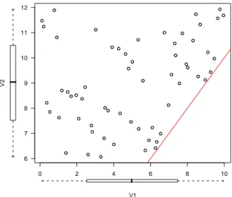
Figure 2 shows the work done on a couple of parameters on which an increasing constraint is enforced, and figure 3 shows the result on a 7-dimensional parameter with a decreasing con-straint. Even if there is good reasons —physical and computational ones— to enforce these constraints, their precise action on the statistical behaviour of a model, in a more general case, is worth studying in future works.

3.6. Estimate indices for the sensitivity analysis

Various estimates of global sensitivity indices are available, among them Standardized Regres-sion Coefficients (SRC), Pearson correlation coeffi-cients, and Partial Correlation Coefficients (PCC). As these three estimates are used in this study, they are briefly presented below.

If the behaviour of Y compared to each parame-ter is overall linear, it is possible to obtain quanti-tative measurements of their influence from the re-gression coefficients bj of the linear regression

con-0 2 4 6 8 10 6 7 8 9 10 11 12 V2 V1

Figure 2: Example of constrained LHS sampling with an increasing constraint. necting Y to X1, X2, . . . , XM: ˆ Y = b0+ M X j=1 bjXj (20)

The standardized regression coefficients are: SRCj= bj· sXj/sY (21)

where sXj and sY are the respective standard

devi-ations of Xjand Y . These coefficients estimate the

variation of the response for a given variation of a parameter Xj and SRCj2 contains the part of the

variance of the output Y which is explained by Xj.

The Pearson product-moment correlation coeffi-cient ρ whose values belongs between −1 and 1 is helpful to estimate the strength of a linear relation-ship between two variables, taking values close than ±1 if the behaviour is linear. Unfortunately, this does not work for multi-variable analysis. In this case, one can build correlation matrices by com-puting the correlation coefficients of each pair of variables. This matrix can be useful to easily de-tect the more important parameters. Finally, ρ2 _is

of the same order than SRC2_.

Here the Pearson correlation coefficients between each Xj and Y is written:

ρXj,Y =

sXjY

sXj · sY

(22) sXjY being the covariance of Xj and Y :

sXjY = 1 N− 1 N X i=1 (xij− xj) (yi− y) . (23)

However, correlation between Y and Xi can be

due to another variable (which is called “tierce cor-relation”). In that case, the SRC and the Pearson correlation coefficients are not pertinent. Partial correlation coefficients (PCC) estimate correlation between two variables when the others belongs con-stant (their effect is removed). The partial correla-tion coefficient between Y and Xiis the correlation

coefficient between Y _{− b}Y and Xi− cXi:

P CCj = ρ_{Y − bY ,Xj− cXj} (24)

where bY is the linear regression of Y when Xjis not

considered and cXj is the linear regression of Xj:

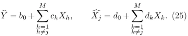
b Y = b0+ M X h=1 h6=j chXh, Xcj= d0+ M X k=1 k6=j dkXk. (25)

In our application case, using these PCC is rele-vant because the monotonic dependences between certain input parameters create some correlations between them. Therefore, SRC and Person coeffi-cients are not protected against tierce correlations.

4. Application to the numerical welding sim-ulation

Two applicative studies are presented below. The first one is an academic 2D study whose aim was to develop and validate the entire process on a medium size problem. The second one is closer to a 3D classical industrial case, more complex and heavier in terms of computation time.

4.1. First application: axi-symmetric heat deposit on a thick disc

4.1.1. Description

The first application is a simple configuration, whose runtime allows several hundred code exe-cution. Thus an axi-symmetrical test is led on a disc of diameter of 160 mm and height of 5 mm in order to investigate residual stresses and distor-tions generated by the heating process. This sim-ulation which is quite similar that used by L. De-pradeux [35] during his doctoral thesis give signifi-cant distortions without melting pool.

4.1.2. Thermal computation

As mentioned before (see section 2), the weak coupling allows to do the thermal computation be-fore the mechanical one. The sensitivity analysis performed here does not concern the thermal part of the computation. Hence we obtain a single thermal loading which will be used in each mechanical sim-ulation. Thermophysical properties (thermal diffu-sivity λ, density ρ, specific heat capacity Cp) must

be described on a whole temperature range from room temperature up to 1200◦_{C. Their numerical}

values presented in the table 2 are taken from liter-ature on the 316L. The heat input is modeled with a standard two-dimensional Gaussian function, and is applied at the center of the disk during a time of 120 s. The supplied power is P = 2500 W.

T (◦C) 20 100 200 300 400 500 600 700 800 900 1000 1200 λ (W/m◦_{C) 14 15.2 16.6 17.9 19 20.6 21.8 23.1 24.3 26 27.3 29.9}

ρ (Kg/m3_{) 8000 7970 7940 7890 7850 7800 7750 7700 7660 7610 7570 7450}

Cp(J/Kg◦_{C) 450 490 525 545 560 570 580 595 625 650 660 677}

Table 2: Thermophysical properties

4.1.3. Mechanical computations

In this study, an elastoplastic with kinematic linear hardening behaviour is considered (see sec-tion 2.2.2). Only 5 mechanical properties are con-sidered: Young’s modulus E, the thermal expansion coefficient α, Poisson’s ratio ν, the yield strength σy

and the hardening modulus H. Their evolutions are discretised for 7 values of temperature. This lead to 7_{× 5 = 35 parameters to be considered in the} Sensitivity Analysis.

4.1.4. Sampling

To illustrate the sampling of the domain, we present in figures 3 and 4 examples for Young’s modulus and for the thermal expansion coefficient. These curves present three randomly selected ma-terials among the 800 created and the bounds of the domain. For the sensitivity analysis process, Young’s modulus is represented by only 7 param-eters, but one should keep in mind that for the mechanical computation, the curve represents truly the considered dependence of this modulus because the algorithm uses intermediate values according to a piecewise linear interpolation.

4.1.5. Numerical aspects

Thermo-mechanical simulations were per-formed using the finite element method and the 11

0.0E +00 5.0E +10 1.0E +11 1.5E +11 2.0E +11 2.5E +11 3.0E +11 0 100 200 300 400 500 600 700 800 900 1000 1100

Figure 3: Example of constrained LHS sampling: Young’s modulus of three randomly selected materials among the 800 created. The upper and the lower curves represent the bounds of the domain for these 7 parameters.

8.0E - 06 1.0E - 05 1.2E - 05 1.4E - 05 1.6E - 05 1.8E - 05 2.0E - 05 0 100 200 300 400 500 600 700 800 900 1000 1100

Figure 4: Example of (unconstrained) LHS sampling: ther-mal expansion coefficient of three randomly selected materi-als among the 800 created. The upper and the lower curves represent the bounds of the domain for these 7 parameters.

Cast3M [36] computer code. Simulations were per-formed with the 2D axi-symmetric FE mesh shown in figure 5. This mesh consists of 506 linear 4-node brick elements with 4 Gauss points. The central zone, where high thermal gradients are expected, is meshed with higher density. All the program settings (resolution algorithm, convergence criteria, time step. . . ) are fixed for all the campaign.

As it can be seen later, 800 mechanical compu-tations have been made. The complete computing time was about 25 hours on a 2004-model personal computer.

Figure 5: Axi-symmetric finite element mesh of the thick disk

4.1.6. Choice of the sample size

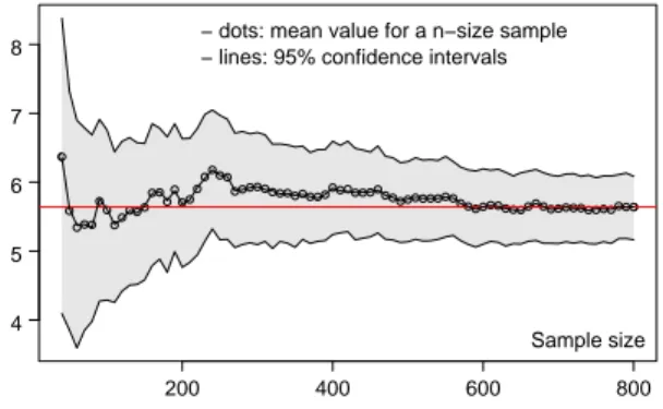
In order to verify the convergence of the Monte Carlo sample of the ouputs, an heuristic visualiza-tion tool is used: the mean value of each model out-put (associated with bootstrap estimates of their 95%-confidence interval) are computed for a grow-ing size set of samples. For example, the behaviour of the stored elastic energy is plotted in figure 6. Similar resuts can be shown for other outputs. They show that beyond 600 samples, the mean value does not vary anymore. This shows that our sampling including 800 elements is representative for this study.

200 400 600 800 4 5 6 7 8 Sample size − dots: mean value for a n−size sample − lines: 95% confidence intervals

Figure 6: Thick disc study: Mean value and 95% confidence interval of the ElastEner output.

4.1.7. Results of the Sensitivity Analysis

For this study, 4 outputs are chosen. The work of plastic deformation during the experiment, the

stored elastic energy at the end of the experiment, the angle of the cone —which is approximately the shape of the deformed disc— at the end of the experiment and the maximum vertical displace-ment of the centre of the disc during the exper-iment. These 4 outputs are named respectively PlastWork, ElastEner, Angle and MaxUZ.

Table 3 presents linear sensitivity coefficients (SRC, Pearson and PCC) of the most important input parameters for the 4 chosen outputs. The squared coefficients are given in order to express the sensitivities in terms of explained variance. Only the ones with a SRC2_{> 0.02 are shown in this}

ta-ble. The good value of R2_{tends to prove the linear}

behaviour of the studied output relatively to the inputs and gives to the sensitivity indices a good validity.

This sensitivity analysis shows that only three parameters among the 35 have a significant effect on the chosen outputs. They are: the yield strength at 20◦_{C (σ}

y20), the thermal expansion coefficient at

20◦_{C (α}

20), and Young’s modulus at 20◦C (E20).

A difference should be noticed for the MaxUZ output, the thermal expansion coefficient at 20◦_C

has more influence than the yield strength at 20◦_C.

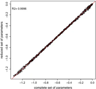
This is not illogical according to the fact that the MaxUZ output is quite particular because it is the only one among the four considered here which takes the maximum value of a quantity over the ex-periment duration. If the vertical displacement is plotted versus time, one must see the displacement goes at a much higher value than his final value. At this moment, temperature values are high all over the disk, giving a predominant weight to the ther-mal expansion coefficient. This is not the case for the three other outputs. It shows that the choice of the output is of great importance in such analysis. The more surprising effect is that only 3 of the 35 parameters have a notable influence. To prove it a posteriori two series of 800 computations are made, the first one with random values for all the parameters (according to the procedure described above), the second with the same values for the three more influential parameters and mean values for the 32 other parameters. As it can be seen on the figure 7, despite the high variability of the con-sidered output, the two series are almost equal (the R2_{is 0.9996). This result means that only 3}

param-eters have to be accuretly measured the 32 other parameters can be taken from classical litterature or arbitrary fixed at a meaning value.

(a) PlastWork output - R2

= 0.8327 σy20 α20 E20 SRC2 _{0.34 0.28 0.15} Pearson2 _{0.43 0.26 0.11} PCC2 _{0.43 0.62 0.31} (b) ElastEner output - R2 = 0.9207 σy20 α20 E20 SRC2 _{0.42 0.32 0.14} Pearson2 _{0.48 0.3 0.12} PCC2 _{0.67 0.8 0.47} (c) Angle output - R2 = 0.9445 σy20 α20 E20 SRC2 _{0.51 0.37 0.054} Pearson2 _{0.52 0.36 0.052} PCC2 _{0.78 0.87 0.33} (d) MaxUZ output - R2 = 0.9361 α20 σy20 other SRC2 _{0.8 0.13 <0.02} Pearson2 _{0.79 0.12} PCC2 _{0.92 0.44}

Table 3: Sensitivity coefficients for the 4 outputs of the thick disc study. −1.2 −1.0 −0.8 −0.6 −0.4 −0.2 0.0 −1.2 −1.0 −0.8 −0.6 −0.4 −0.2 0.0

complete set of parameters

reduced set of parameters

R2= 0.9996

Figure 7: Thick disc study: Comparison of the output An-glefor a N = 800 LHS/cLHS sample between computations firstly made with a complete set of parameters and secondly with only the three more influential parameters (the 32 oth-ers are fixed to their mean value).

4.2. Second application: welding line on a thin plate

4.2.1. Description

A square plate of side 250 mm and thickness 1.6 mm receives a line heat deposit simulating the use of a moving TIG source. The heat deposit is done over a limited path in the x-direction and the plate is clamped at its x = xmaxside. This is done

to limit computation time while keeping represen-tative of a welding experiment.

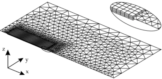
According to the symmetry of the problem, only a half side of the plate is meshed. To reduce some more the computation time, a mixed mesh is used, see figure 8. This mesh is done with 3D elements in the heat deposit zone, and shell elements for the rest of the plate. So the problem is correctly mod-elised: the 4 layers of 3D elements in the heat de-posit zone are able to manage strong thermal gra-dients and the viscoplasticity behaviour, unless the shell elements are sufficient to describe the thermo-mechanical bending of the rest of the plate because the viscoplasticity is absent and the thermal varia-tion in the z-direcvaria-tion is moderate.

This mesh is made up of 3934 elements, 2760 8-nodes hexahedrons and 1174 3-8-nodes DKT shell el-ements. Special conditions are prescribed at the interface between solid and shell elements to verify forces equilibrium and heat flux balance.

The heat deposit is modelised by a volumetric heat source model proposed by Goldak [37]. The seven parameters used by this model are classically adjusted by inverse methods from experiment re-sults.

The mechanical model is the viscoplastic model described in section 2.2.2 with 8 parameters. In or-der to limit the computation time, each of the 8 parameters temperature evolutions are discretised only for the 5 temperature values: 20, 500, 800, 1100 and 1300 ◦_{C. This leads to 40 input}

parame-ters for the sensitivity analysis, which is comparable to the precedent study.

However, this 3D finite element model is bigger than the above 2D disk model: time computation for one set of parameters is now about 6 hours. As a 500 materials sampling had been considered for this study, the total time computation is estimated to 125 days. Fortunately, this type of study, which is by nature highly parallelizable, was made using several computers.

Other numerical aspects are identical to those de-scribed above.

Figure 8: Thin plate study: Mesh of the plate.

4.2.2. Sensitivity analysis

In this study, it was decided to consider only dis-placements outputs. Three points were chosen on the plate and their vertical displacement uz were

followed up during each experiment. As their evo-lutions were similar, only one of them will be con-sidered here. This point P is the (xmin, ymax)

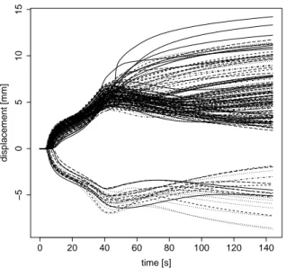
cor-ner, at the opposite of the clamped side. Only final values are taken for the sensitivity analysis, but the evolution is particularly interesting as can be seen in figure 9.

This figure shows, for all the experiments, the time evolution of the uzdisplacement of the

consid-ered point. It can be seen that some experiments give “opposite” results. From a mechanical point of view, this phenomenon seems to resemble a buck-ling instability. The structure hesitates to bend in a direction or in the opposite direction. For a very small change in some properties, the final state can be very different. As the purpose of this study was to implement the sensitivity analysis, this partic-ular aspect is no more developed here, even if it seems particularly interesting. So, we choose to ignore these “opposite” results because they can produce strong artificial sensitivity related to this —presumed— elastic instability and would lead to bad results. That points out the great importance of output choice.

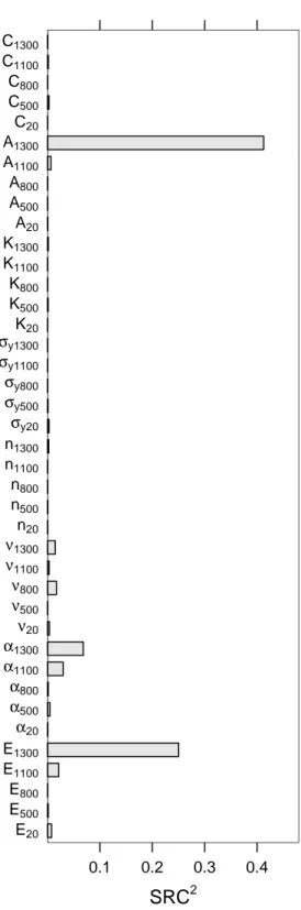
The result of the sensitivity analysis is presented on figure 11. This figure shows that the result is different from the precedent study except from the fact that three of the forty parameters share 90 percent of the variability of this output. In this case however, the most influential parameters are high-temperature values of the plastic strain coef-ficient A1300 Young’s modulus E1300 and the

ther-mal expansion coefficient α1300. Numerical values

are given in table 4.

0 20 40 60 80 100 120 140 −5 0 5 10 15 time [s] displacement [mm]

Figure 9: Thin plate study: Displacement curves for each material simulated (vertical displacement on the point P ).

Figure 10: An example of deformed plate

precedent study is due to the nature of the problem. This will be discussed in the section 4.3.

Final displacement zP — R 2 = 0.9004 A1300 E1300 α1300 SRC2 0.41 0.25 0.068 Pearson2 0.34 0.18 0.24 PCC2 0.73 0.63 0.062

Table 4: Thin plate study: Sensitivity coefficients for the final z-displacement of the point P .

4.3. Discussion

The two studies gave different results. The first one has shown that low temperature parameters σy20, α20, and E20 were the most important. The

second study leads to a different ranking, the most influential are the high temperature parameters: A1300, E1300 and α1300.

These two problems are different for many rea-sons. Firstly, the model is elasto-plastic in the disk study and elasto-viscoplastic in the plate study. As the sets of parameters are not the same in the two studies, even the common parameters may have dif-ferent relative importance in each model. Secondly, the nature of the two studies strongly differs. The disk is thick and solicited at his centre. It is a very rigid structure. When the disk has cooled down, only a small plastic zone at the centre struggles against the rest of the disk which remains elas-tic. In the plate case, the plate is thin and easy to bend, and the solicitation is more extended than a point, it is a line. This is a less rigid case. Fur-ther, because the plate is thin, all the heated zone has reached high temperatures, which may explain the high temperature parameters ranking.

These two studies show that the validity of the sensitivity analysis result is attached to the consid-ered system or model. General conclusions must be very carefully tested before their confirmation. They also show the power of the sensitivity analysis tool for numerical simulations like welding, allowing strong reduction of models —provided the respect of the precaution mentioned above.

5. Conclusion

The present paper has suggested an efficient pro-cedure to perform a sensitivity analysis in welding simulation. The study was limited to the sensitivity to mechanical parameters. The unsteady thermal 15

SRC

Figure 11: Thin plate study: Final z-displacement of the point P . Sensitivity indexes SRC2

for the 40 inputs (8 me-chanical properties discretized for 5 temperature values)

response was computed only once, and the temper-ature field evolution used as thermal load in me-chanical computations.

The sensitivity analysis was chosen to be of global type, in order to covers the entire steel domain with-out the drawbacks of local methods. Inputs are the parameters of the mechanical models, each of them discretised into values for different temperatures. This leads to a set of 35 (40) inputs, which is quite a lot dealing with sensitivity analysis. Outputs are classical mechanical observables like displacements, stresses or energy. A LHS technique generates a sample of input parameters set, each of them rep-resenting a virtual steel.

Physical considerations have lead to modify the classical LHS technique to enforce monotonic tem-perature variation for some of the mechanical pa-rameters. This constrained LHS technique pro-posed in [34] was used to sample these particular mechanical parameters, as a classical LHS tech-nique was used for the others.

Numerical welding simulations are performed for all the virtual materials of the sample, and the sen-sitivity analysis is done. Sensitivity indices like Standardized Regression Coefficient (SRC), Pear-son correlation coefficients and Partial Correlation Coefficients (PCC) are computed for all input pa-rameters.

Two practical studies were achieved. These two studies differ in the welding configuration and con-sidered mechanical models (one is elastoplastic with 35 parameters and the other is elastoviscoplastic with 40 parameters). The results of the two sen-sitivity analysis are different but, a surprising fact is that, in both cases, only 3 of the 35 (40) input parameters explains 90% of the outputs variability. To verify a posteriori this result, a sample of a 800 materials is generated. A duplicata of this sam-ple is made, keeping the random values for the 3 most important parameters and giving mean values to all the other parameters. Two series of computa-tions were performed, one for the native sample and one for the degenerated one. Then outputs were compared for both corresponding materials. Which is remarkable is, despite the high variability of the considered outputs, both couples of corresponding materials had given very near results.

Sensitivity analysis has provided answers to what we consider one of the probable frequently asked questions regarding welding simulation: for a given welding problem, which properties must be mea-sured with a good accuracy and which ones can be

simply extrapolated or taken from a similar ma-terial? Indeed, a Global Sensitivity Analysis per-formed onto a representative numerical model is able to find the most influent input parameters. Considering the preliminary results of this work it is permitted to think that they are very few compared to all the required inputs. That may avoid doing numerous difficult and expensive experiments to de-termine precisely parameters whose mean value is proved to be sufficient.

Finally, a new simulation methodology is pro-posed, including four sequential steps: Firstly the problem needs to be characterized (nature, mate-rial, models, inputs and outputs, domain, etc.) and a representative numerical model is built. Secondly, a Global Sensitivity Analysis is done, which leads to the ranking of input sensitivities. Then the most influential parameters are carefully measured —if possible— on the considered material, other mate-rial properties are fixed to probable values (repre-sentative of the material family for example). Nu-merical simulations can now be performed. Three advantages could be expected: a substantial reduc-tion of the amount of experiments and the induced financial and time economies, more accurate results because precise data are considered for the most influential parameters, the physical meaning of the sensitivity analysis results can lead to a better un-derstanding of phenomena.

References

[1] A. Loredo, B. Martin, H. Andrzejewski, and D. Grevey. Numerical support for laser welding of zinc-coated sheets process development. Applied Surface Science, 195(1-4):297–303, July 2002.

[2] B. Martin, A. Loredo, D. Grevey, and A.B. Vannes. Numerical investigation of laser beam shaping for heat transfer control in laser processing. Lasers in Engineer-ing, 12(4):247–269, 2002.

[3] J. K. Hepworth. Finite element calculation of residual stresses in welds. Num. Meth. Non-Lin. Prob., pages 51–60, 1980.

[4] P. Tekriwal and J. Mazumder. Transient and Resid-ual Thermal Strain-Stress Analysis of GMAW. Journal of Engineering Materials and Technology, 113:336–343, 1991.

[5] L.E. Lindgren. Finite element modeling and simulation of welding part 3 : efficiency and integration. Journal of thermal stresses, 24:305–334, 2001.

[6] J. Canas, R. Picon, F. Pariis, A. Blazquez, and J. C. Marin. A simplified numerical analysis of residual stresses in aluminum welded plates. Computers & Structures, 58(1):59–69, January 1996.

[7] G. Chen, X. Xu, C. C. Poon, and A. C. Tam. Experi-mental and 2D numerical studies on microscale bending

of stainless steel with pulsed laser. Journal of Applied Mechanics, 66:772–779, 1999.

[8] Q. Y. Shi, A. L. Lu, H. Y. Zhao, P. Wang, A. P. Wu, Z. P. Cai, and Y. P. Yang. Effects of material prop-erties at high temperature on efficiency and precision of numerical simulation for welding process, volume 2 of ISBN: 0965700135, chapter Advances in Computa-tional Engineering & Sciences, pages 655–660. 2000. [9] K. Abdel-Tawab and A. K. Noor. Uncertainty analysis

of welding residual stress fields. Computer Methods in Applied Mechanics and Engineering, 179(3-4):327–344, September 1999.

[10] X. K. Zhu and Y. J. Chao. Effects of temperature-dependent material properties on welding simulation. Computers & Structures, 80(11):967–976, May 2002. [11] J. Song, J. Y. Shanghvi, and P. Michaleris.

Sensitiv-ity analysis and optimization of thermo-elasto-plastic processes with applications to welding side heater de-sign. Computer Methods in Applied Mechanics and En-gineering, 193(42-44):4541–4566, October 2004. [12] M. Petelet and O. Asserin. Influence des param`etres

d’un mod`ele ´elastoplastique sur les distorsions calcul´ees par simulation num´erique d’une op´eration de soudage. In Congr`es Francais de la M´ecanique, 2005.

[13] C. Schwenk, M. Rethmeier, K. Dilger, and V. Michailov. Sensitivity analysis of welding simulation depending on material properties value variation (submitted). In Mathematical Modelling of Weld Phenomena, vol-ume 8, Graz, 2007.

[14] D. A. Tortorelli and P. Michaleris. Design sensitivity analysis : Overview and review. Inverse Problems in Engineering, 1:71–103, 1994.

[15] M. D. Morris. Factorial sampling plans for preliminary computational experiments. Technometrics, 33(2):161– 174, May 1991.

[16] J. C. Helton. Uncertainty and sensitivity analysis tech-niques for use in performance assessment for radioac-tive waste disposal. Reliability Engineering and System Safety, 42:327–367, 1993.

[17] A. Saltelli, T. H. Andres, and T. Homma. Sensitiv-ity analysis of model output: An investigation of new techniques. Computational Statistics & Data Analysis, 15:211–238, 1993.

[18] J.P.C. Kleijnen. Sensitivity analysis and related anal-yses: a review of some statistical techniques. Journal of Statistical Computation and Simulation, 57:111–142, 1997.

[19] B. Iooss, F. Van Dorpe, and N. Devictor. Response surfaces and sensitivity analyses for an environmental model of dose calculations. Reliability Engineering & System Safety, 91:1241–1251, 2006.

[20] A. Saltelli, K. Chan, and E. M. Scott. Sensitivity Anal-ysis. Wiley, 2000.

[21] A. Saltelli, S. Tarantola, F. Campolongo, and M. Ratto. Sensitivity Analysis in Practice: A Guide to Assessing Scientific Models. WILEY, 2004. 232 pages.

[22] K. T. Fang, R. Li, and A. Sudjianto. Design and Mod-eling for Computer Experiments, volume 6. Chapman & Hall/CRC Computer Science & Data Analysis, 2005. [23] E. De Rocquigny, N. Devictor, and S. Tarantola, edi-tors. Uncertainty in industrial practice. Wiley, 2008. [24] B. Iooss. Manuel utilisateur du logiciel SSURFER

V1.2 : programmes en R d’analyses d’incertitudes, de sensibilit´es, et de construction de surfaces de r´eponse. Technical report, NOTE TECHNIQUE CEA, 17

DEN/CAD/DER/SESI/LCFR/NT DO 6 08/03/06, 2006.

[25] R Development Core Team. R: A Language and Envi-ronment for Statistical Computing. R Foundation for Statistical Computing, Vienna, Austria, 2006. ISBN 3-900051-07-0.

[26] P. Pilvin. Identification des param`etres de mod`eles de comportement. In MECAMAT, pages 155–164, Be-san¸con, 1988.

[27] J.L. Chaboche. A review of some plasticity and vis-coplasticity constitutive theories. International Journal of Plasticity, 24(10):1642 – 1693, 2008. Special Issue in Honor of Jean-Louis Chaboche.

[28] L. E. Lindgren. Modelling for residual stresses and de-formations due to welding - Knowing what isn’t neces-sary to know. In H. Cerjak, editor, Mathematical Mod-elling of Weld Phenomena, volume 6, 2002. presented in Graz, Austria, Oct 2001.

[29] A. Saltelli, M. Ratto, T. Andres, F. Campolongo, J. Cariboni, D. Gatelli, M. Saisana, and S. Taran-tola. Global Sensitivity Analysis: The Primer. WILEY, 2008. 304 pages.

[30] D. G. Cacuci. Sensitivity theory for non-linear systems. Journal of Mathematical Physics, 22, 1981.

[31] T. Turanyi. Sensitivity analysis of complex kinetic sys-tems. tools and applications. Journal of Mathematical Chemistry, 5(3):203–248, September 1990.

[32] M. D. Mc Kay, W. J. Conover, and R. J. Beckman. A comparison of three methods for selecting values in the analysis of output from a computer code. Technomet-rics, 21(2):239–245, 1979.

[33] J. C. Helton and F. J. Davis. Latin hypercube sampling and the propagation of uncertainty in analyses of com-plex systems. Reliability Engineering & System Safety, 81(1):23–69, July 2003.

[34] M. Petelet. Analyse de sensibilit´e globale de mod`eles themom´ecaniques de simulation num´erique du soudage. PhD thesis, University of Burgundy, 2007.

[35] L. Depradeux. Simulation num´erique du soudage -Acier 316L. Validation sur cas tests de complexit´e croissante. PhD thesis, INSA Lyon, 2003.

[36] Cast3M. CEA Finite Element software, 2007.

[37] J. Goldak, A. Chakravarti, and M. Bibby. A new finite element model for welding heat flow in welds. Metal-lurgical Transaction B, 15B:299–305, June 1984.