Objectives
Development, implementation and validation of an analytical method to quantify the secondary structure of proteins in water using Fourier-transform infrared spectroscopy.
Methods | E xperien ces | Resu lts
The secondary structure of proteins is extracted from the shape of the amide I band (1600-1700 cm-1). Infrared spectra of proteins in water at 5% w/V concentration were recorded and corrected for water and water-vapour absorption. The latter was minimized by purging using nitrogen. Second-derivative spectra were calculated from the smoothed corrected spectra using a five points Savitsky-Golay algorithm. The various peaks present in the second-derivative spectra were integrated and attributed to the different secondary-structure motives: α-helices, β-sheets and β-turns.
The developed method yielded reproducible results for the ten model proteins tested. The proportions of the different secondary-structure motives were in close agreement with previous reports using FTIR spectroscopy and usually corresponded to experimental values derived from X-ray structures.
Objectifs
Développement, implémentation et validation d’une méthode analytique pour quantifier la structure secondaire des protéines dans l’eau en utilisant la spectroscopie infrarouge à transformée de Fourier.
Méthodes | E xpérie nces | Résultats
La structure secondaire des protéines est extraite de la forme de la bande amide I (1600-1700 cm-1). Les spectres infrarouge de diverses protéines dans l’eau à 5% m/V ont été obtenus et corrigés pour éliminer l’absorption de l’eau et de la vapeur d’eau. Cette dernière a été minimisée par une purge d’azote. Les spectres de la seconde dérivée ont été calculés depuis le spectre affiné et corrigé en utilisant l’algorithme de Savitsky-Golay à cinq points. Les différents pics présents dans le spectre de la seconde dérivée ont été intégrés et attribués aux différents motifs de structure secondaire : hélices α, feuillets β et boucles β.
La méthode développée donne des résultats reproductibles pour les dix protéines modèles testées. Les proportions des différents motifs de structure secondaire sont concordants avec des publications utilisant la spectroscopie FTIR et correspondent aux valeurs expérimentales dérivées des structures aux rayons X.
Analysis of protein secondary structure by FTIR
Graduate Ruffieux Bastien
Bachelor’s Thesis | 2 0 1 2 | Degree course Life Technologies Field of application Analytical chemistry Supervising professor Prof. Dr Segura Jean-Manuel [email protected]
Partner
Picture 300 dpi 6 x 9cm
Photo edited using Photoshop
HES-SO Valais | School of Engineering Route du Rawyl 47
1950 Sion
Tél. 027 606 85 11 URL www.hevs.ch
1
Sommaire
1 Introduction ... 2
1.1 Protein secondary structure ... 3
1.1.1 Secondary structure motives assignment ... 4
2 Material ... 6 2.1 Proteins ... 6 3 Method... 7 3.1 Optimisation ... 7 3.1.1 Purge ... 8 3.1.2 Number of scan ... 11 3.1.3 Resolution ... 12 3.1.4 Gain ... 13 3.1.5 Concentration ... 15 3.2 Data processing ... 17 3.2.1 Water correction ... 18 3.2.2 Vapour correction ... 19 3.2.3 Smoothing ... 21 3.2.4 S-G 2nd derivative... 22 3.2.5 Fourier self-deconvolution ... 23 3.3 Final method ... 24 4 Results ... 25 5 Discussion ... 29
5.1 Water and vapour subtraction ... 29
5.2 Vapour subtraction ... 29
5.3 Results ... 30
6 Conclusion ... 31
7 Bibliography ... 32
2
1
Introduction
In biochemistry, proteins are very complex molecules due to a highly complicated structure and an even more complicated mechanistic functionality. Proteins are the legacy from billions of years of evolution, fail and success (Alberts B., 2002). A protein is defined by two major aspects, its linear structure — the primary one — composed in a chain of amino acids, and its three dimensional structure — and its secondary, tertiary and quaternary structure.
The Primary structure is made of a long chain of amino acids. There are 20 types of amino acids, each with different chemical properties which bond it to its neighbour by a covalent peptide bond. Each protein has a specific sequence of amino acids.
Figure 1: Protein primary structure and peptide bond
If the primary structure is essential to the proper working of a protein, the secondary structure is as important but harder to define and analyse.
3
1.1
Protein secondary structure
Protein secondary structure is the general three-dimensional form of local segments of proteins. It doesn’t describe the atomic position in three-dimensional space which is the tertiary structure.
Secondary structure motives are defined by the hydrogen bond stabilising its structure between carbonyl and nitrogen of amino acids. H-bond generates specific dihedral angles that determine the orientation and secondary structure motives. Secondary structure can then be determined as the repetition of H-bonds. In vibrational spectroscopy such as infrared ones, in general, H-bonds influence the amide I band, which is specific to the C=O bond vibration. (Barth, 2007)
A method to define the protein secondary structure motives is the DSSP one (Kabsch W., 1983). This method defines the secondary structure motives by the electronical density of the hydrogen bond. A hydrogen bond is identified if E in the following equation is less than -0.5kcal/mol.
= ∗ ∗ 1 + 1 − 1 − 1 ∗
1.1.1 Secondary structure motives assignment A hydrogen bond on the C=O create
a shift of the carbonyl peak. Usually, a different motives, α-helix, β-sheet and
The α-helix is a group of motives containing 3 motives have the same global
between the H-bond. The helix is a s
amino acid i makes a bond with the amino acid and i to i+5, π-helix. Figure 2 shows an example of
Figure 2: alpha helix motive of protein. Yellow: H
The β-sheet is a strand connected laterally by H depending of the alignment of the two
Figure 3: antiparallel and parallel
beta-4
Secondary structure motives assignment
hydrogen bond on the C=O creates a modification of the vibration. Concretely it . Usually, an H bond makes a negative shift.
sheet and β-turn.
helix is a group of motives containing 310 helix, α-helix and
π-motives have the same global appearance; the only difference is the number of amino acids The helix is a spiral where each amino acid makes
a bond with the amino acid i+3, then a 310 helix is formed,
shows an example of alpha helix.
: alpha helix motive of protein. Yellow: H-bond
connected laterally by H-bond. It can either be parallel or antiparallel, depending of the alignment of the two protein parts participating on the β
-sheet
Concretely it generates a negative shift. There are three
-helix. These three the number of amino acids piral where each amino acid makes an H-bond. If an helix is formed, i to i+4, α-helix
It can either be parallel or antiparallel, participating on the β-sheet.
5
β-turn are a single H-bond between two amino acid separated by a few, 1 to 5 peptide bonds. In fact, they are single α-helix or β-sheet. Figure 4 shows a beta turn i to i+3.
Figure 4: beta turn i to i+3
All these secondary structure motives induced a shift of the amide I band due to the hydrogen bond. The shifts are specific to each structure and a table can be made to assign each peak in the amide I band to a motive. Table 1 shows these specific assignments.
Table 1: assignment of peak frequency to secondary structure motives frequency assignment 1624 β-sheet 1627 β-sheet 1633 β-sheet 1638 β-sheet 1642 β-sheet 1648 Random coil 1656 α-helix 1663 310-helix 1667 β-turn 1675 β-turn 1680 β-turn 1685 β-turn 1691 β-sheet 1696 β-sheet
Being able to analyse and quantify the secondary structure is very important. To do its job, a protein must be correctly folded. In most biochemical domain, proteins are the most used type of molecule. There are denaturized, renaturized and must work well after the process. When synthesizing a protein, the folding is a major part of the process.
To be sure that a protein is functional, a method must be created to certify the folding of the protein.
6
2
Material
—Nicolet 5700 FTIR, Thermo —OMNIC Software version 1.26
—Spacer MYLAR 0.006 mm, Portmann Instruments AG —Nitrogen 4.5, Pangas
—MATLAB Software version 7.10.0.499 (R2010a)
2.1
Proteins
—Lysozyme, from chicken egg white, SIGMA, L6876
—Concanavalin A, from Canavalia ensiformis, SIGMA, L7647 —Ribonuclease A, from bovine pancreas, SIGMA, R5500 —Pepsin, from porcine gastric mucosa, SIGMA, P6887 —Hemoglobin, from bovine blood, Fluka, 51290 —Myoglobin, from horse heart, SIGMA, M1882 —Cytochrome C, from equine heart, SIGMA, C7752 —Trypsin, from bovine pancreas, SIGMA, T8003
7
3
Method
3.1
Optimisation
Based on the work of Dong (Dong A., 1990) and Kong (Kong J., 2007), initial parameters were known and optimized to reduce the analysis time. A nitrogen purge is also applied to reduce absorption of water and water vapour in the amide I band (1600-1700 cm-1) and make the subtraction of residual vapour easier. (Pelton J. T., 2000)
Optimized parameters of the Fourier transform infrared spectroscopy are the number of scans, the resolution and the gain through the setting of the aperture. Some analysis parameters are optimized as well, nitrogen purge, protein concentration and all the data processing.
The highest difficulty of this analysis is the width absorption band of water appearing between 1600 and 1700 cm-1. Most of the optimizations are made to reduce the effect of water and vapour on the amide I band.
Another way to eliminate water absorption is to use D2O instead of water for the analysis.
This method has the advantage of suppressing water absorption at 1650 cm-1 and allowing in the same case the use of cells with much longer path length. A much longer path length also allows a smaller concentration of protein, which is better for hydrophobic protein. But some other things must be considered. First of all, protein structure can slightly change in D2O due
to the difference of weight between deuterium and hydrogen that will change the properties of hydrogen bond. To avoid a protein with both hydrogen and deuterium in it, a study on deuterium-hydrogen transfer must be done. So analysing protein in D2O has some good
advantage but also some disadvantage.
8 3.1.1 Purge
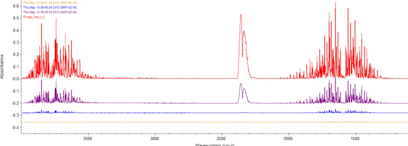
Purging ambient air by nitrogen allows an easier subtraction of the water vapour spectrum. The vapour appears as a high number of peaks between 1350 and 2000, absorbing right in the area of the amide I band. Two parameters can be improved for the purge. The duration of the purge and the output pressure that corresponds to the flow of nitrogen. The duration can easily be determined as the time when no changes are observed to the absorbance of the specific peaks of vapour with more time of purging. Figure 5 shows the evolution of the purge in time. The spectrums are in absorbance versus a 10 minute purge.
Figure 5: relative absorbance of vapour at different time of purging versus a 10 minute purge. Red: 0 minute purge. Purple: 1 minute purge. Blue: 5 minute purge. Yellow: 9 minute purge.
After 10 minutes, no significant changes are visible. That set the optimal purge time to 10 minutes.
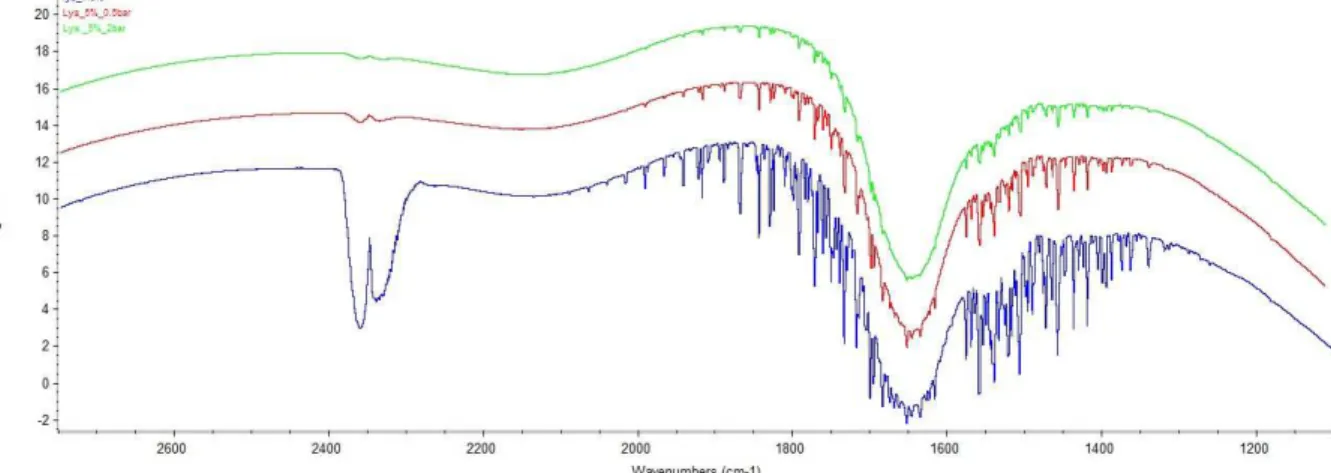
The second parameter is less evident to determine and both efficiency of the purge and high needed flow of nitrogen must be considered. The Figure 6 shows that by using a simple nitrogen purge, it is easy to considerably reduce the impact of the vapour, as disturbing impurities, in the area of analysis.
9
Figure 6: Spectrum of lysozyme with three different purges. Light green: 10 min of output pressure of 2 bar nitrogen. Red: 10 min of output pressure of 0.5 bar nitrogen. Dark blue: no nitrogen purge
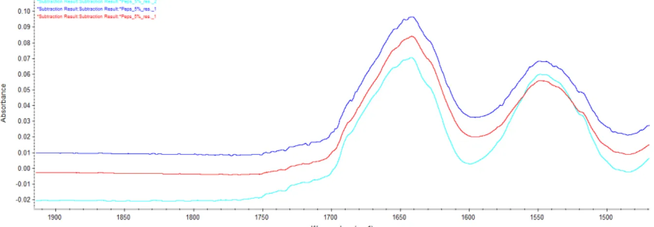
An important effect can be shown even with a small purge. At 0.5 bars, the peaks are already highly reduced but 2 bar shows a significant improvement that can be observed only after the subtraction of the water and the vapour. Figure 7 shows the spectrum of lysozyme after the subtraction.
Figure 7: Spectrum of lysozyme with three different purges after subtraction of water and vapour. Red: 2 bar purge. Blue: 0.5 bar purge. Green: without purge
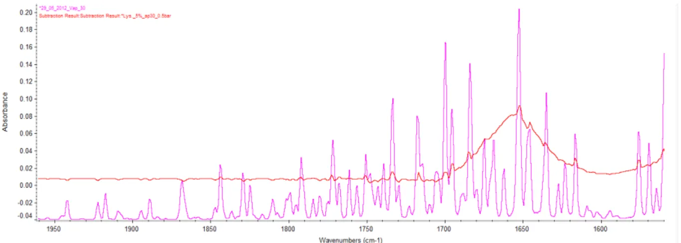
The spectrum is now clean for the spectrum with the 2 bar purge. But we can see that the two other spectrums had a lot of peaks remaining from the vapour. It’s not possible to clean them more due to the presence of positives and negatives peaks. Subtracting the vapour more or less will only make some other peaks appear while some peaks will disappear. The area between 1700 and 1900 cm-1 in the green spectrum clearly demonstrate this problem with a lot of peaks specific to the vapour. This can be observed on Figure 8 by superposing the spectrum to the vapour spectrum.
10
Figure 8: Clean spectrum of lysozyme without purge and spectrum of vapour. Red: lysozyme spectrum. Violet: Vapour spectrum
All these observations made the parameters of an optimal purge set to 10 minutes and 2 bar of output pressure. Having a better purge will only give really small changes with a higher analysis price. Even with a 2 bar purge, with 10 minutes purge and 4 minutes analysis, that cost about 20 bar of a 50l canister of 200 bar nitrogen at 60 CHF (2012/08/01), about 6 CHF of nitrogen per analysis. But we must also consider that we can’t make more than 10 analysis per canister and it’s better not to stack a lot of high pressure nitrogen.
11 3.1.2 Number of scan
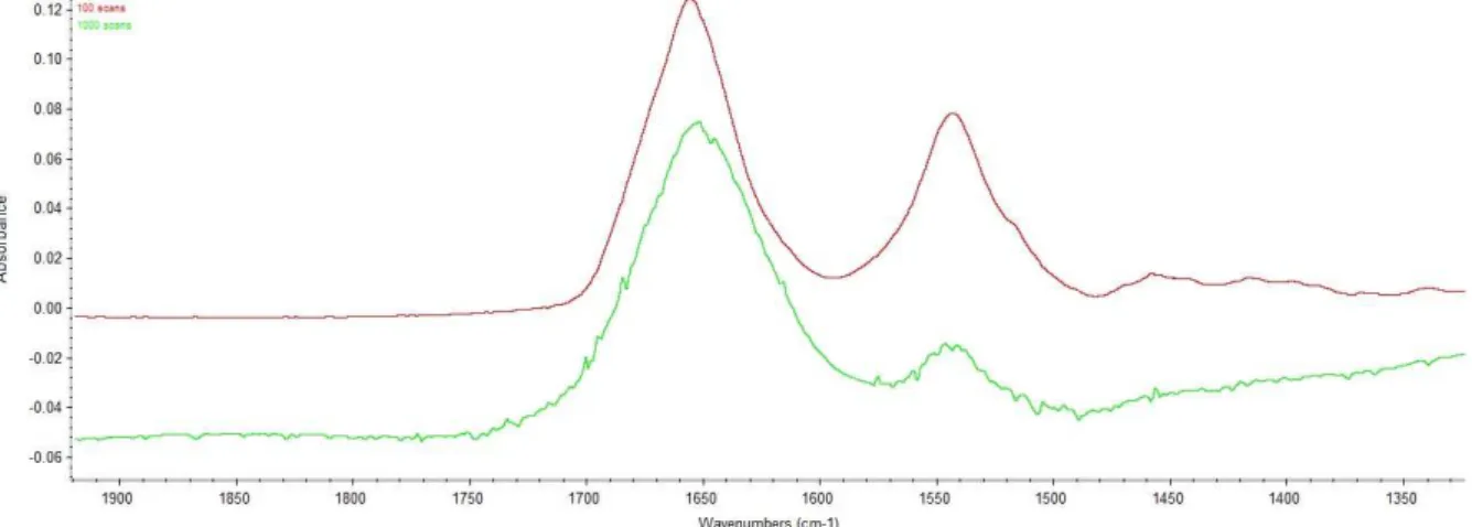
Two different number of scan are tried, 100 scans and 1000 scans. It seems that 1000 scans is the most used, but due to the high necessary volume of nitrogen, it would be better to use a smaller number of scan. After trying both, a smaller number of scans appears to demonstrate better results. This is shown on Figure 9.
Figure 9: Comparison between a 100 scans and 1000 scans analysis. Red: Lysozyme with 100 scans. Light green: Lysozyme with 1000 scans
Most people used a higher number of scans (Dong A., 1990) (Kong J., 2007) but we saw that with our device and our parameters, it gives better result with a smaller number of scans. The reason is hard to explain because in normal cases, a higher number of scans must reduce the background noise. We can only make the supposition that the noise we detect with a higher number of scans comes from impurities in water or in protein and appear when stacking a high number of analysis. But something like this is hard to tell due to the two subtractions made before. These noises can occur in both the subtraction of water and subtraction of vapour.
As the experimental analysis shows, a number of scans of 100 is preferable to a higher number but the reason is only that we observed it. To pull the experiment in extreme way, a number of scan of 8 has been tried to be sure that it’s necessary to have a high number of scan and the result is as expected that with a really small number of scan, the background can’t be subtracted. The experiment has also been made on pepsin and cytochrome C with the same results.
12 3.1.3 Resolution
By changing the resolution, the number of data in the spectrum become higher or smaller. With a resolution of 2, the spectrum has about one point by cm-1 and with a resolution of 1, two points by cm-1. Figure 10 shows the difference between 2 cm-1 resolution and a 1 cm-1 resolution after the smoothing.
Figure 10: Comparison between a resolution on the FTIR of 1 and 2. Cyan: resolution of 2, 9 points smoothing. Red: resolution of 1, 17 points smoothing. Blue: resolution of 1, 9 points smoothing
The first thing to see is that with a higher number of points, keeping the same smoothing factor (c.f 3.2.3 smoothing) makes no sense. Even if with a 9 points smoothing with a resolution of 1 we’ve got quite a similar spectrum, we need to apply a smooth with two times more points — seventeen in that case — to get a really similar spectrum. The same reasoning is made for the 2nd derivative in Figure 11.
Figure 11: Comparison between 1 and 2 cm-1 resolution after 2nd derivative. Red: resolution of 2, 5 points derivative. Green: resolution of 1, 9 points derivative
13
Both resolutions show clean spectrum for pepsin. Both give same results on secondary structure determination. One advantage of a 2 cm-1 resolution is that the base line is easier to see because already flat. But the 1 cm-1 resolution gives a cuter spectrum with more curves due to the higher number of data. This has absolutely no analytical value but is not to be neglected for a presentation. In conclusion, a resolution of 2 cm-1 is better mostly because it is cheaper due to a smaller analysis time.
3.1.4 Gain
The gain of the infrared device depends directly on the aperture and the sample. For a sample of a 5 % w/V protein, a gain of 1 can be obtained with an aperture of about 30. The gain is calculated by the OMNIC software. Due to some difference between analysis proteins, the gain can’t be assured with a single aperture.
To show that the aperture has no significant impact on this analysis, the biggest aperture allowed by the software has been tested. But to keep a simple operative procedure, instead changing the aperture for each protein, an aperture of 30 is used in each case.
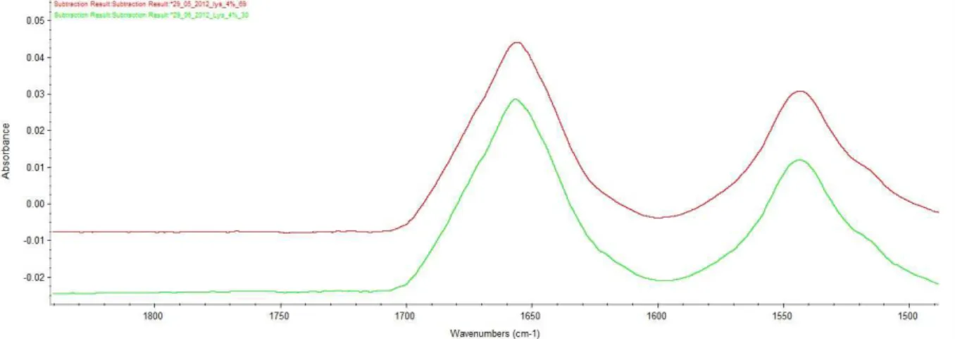
Figure 12 shows the spectrums of lysozyme obtained with an aperture of 30, the best theoretical gain, and 69, the maximum gain of the software.
Figure 12: effect of aperture on lysozyme analysis. Red: aperture of 69. Green: aperture of 30
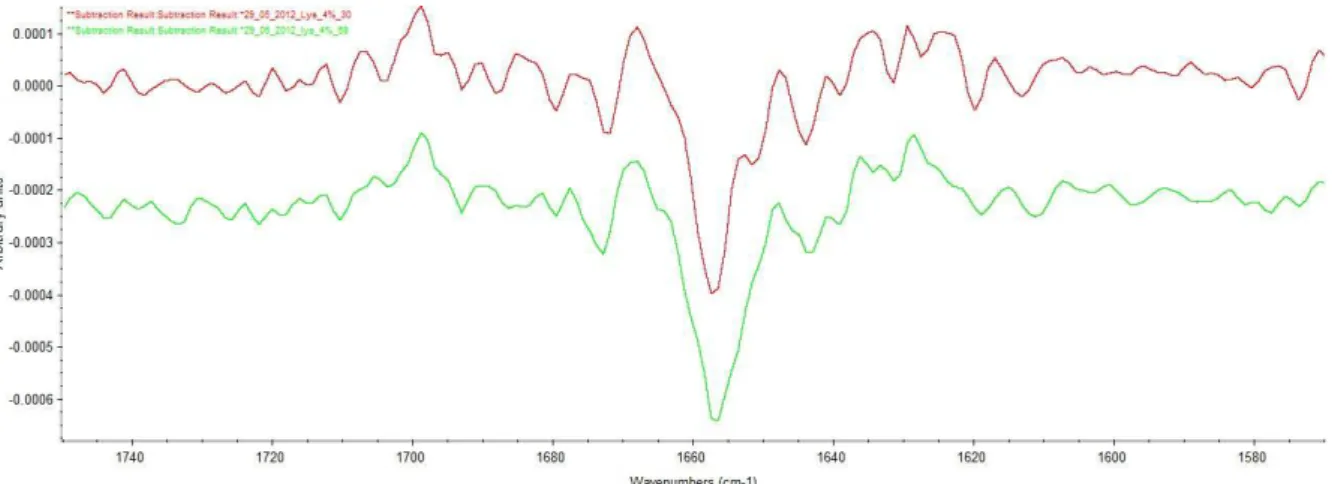
The aperture has no visible impact on the spectrum after modification. But after the Savitzky-Golay 2nd derivative, a difference can be observed. Figure 13 shows these same spectrums after the 2nd derivative.
14
Figure 13: effect of aperture on lysozyme analysis after S-G 2nd derivative. Red: aperture of 30. Green: aperture of 69
After applying the S-G 2nd derivative, some differences appear. If the two spectrums show no significant differences relatively to the desired precision of the analysis, peaks are better defined with a better gain (aperture of 30, red spectrum) than with a bigger aperture (aperture of 69, green spectrum).
With a high difference of aperture, the differences on the final spectrums are smaller. After this conclusion, it appears that keeping an aperture of 30 for all proteins without any distinction won’t change the final analysis.
15 3.1.5 Concentration
Proteins are high price molecules when bought and when synthesized, therefore it’s hard to get a high concentration. To get an easy analysis process, having a single concentration working for most proteins is a bonus. Based on the work of Dong, Huang and Caughey[ (Dong A., 1990)], a concentration of 5 % w/V is used. But due to the low dissolution of some protein in water, it could be good to use a low concentration.
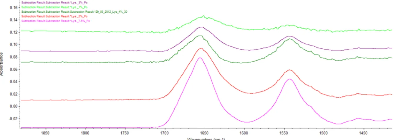
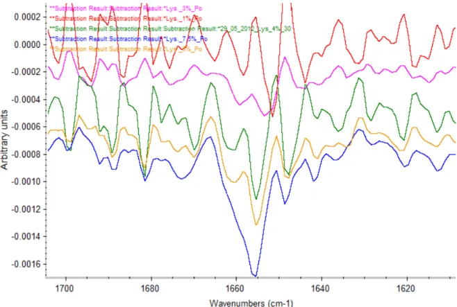
Lower concentrations have been tried. Figure 14 shows the spectrum of lysozyme at 7.5, 5, 4, 3 and 1 % w/V after subtracting the water and vapour.
Figure 14: spectrum of lysozyme at different concentration. Light green: lysozyme 1%. Violet: lysozyme 3%. Dark green: lysozyme 4%. Red: lysozyme 5%. Pink: lysozyme 7.5%
The comparison between the spectrums shows that a higher concentration gives a better spectrum. Amide I band is more intense and the noise is highly reduced. But the amide I band is still present even with low concentration so to know the limit concentration the process must be conducted to the end and we must observe the 2nd derivative spectrum.
Figure 15 shows the same different concentration after a 9 points S-G smoothing followed by a 5 points S-G 2nd derivative.
16
Figure 15: Comparison between different concentrations after 2nd derivative. Red: lysozyme 1%. Pink: lysozyme 3%. Green: lysozyme 4%. Yellow: lysozyme 5%. Blue: lysozyme 7.5%
With small concentration, we can see most of the principal peaks. But it is not possible to get a good base line and most of the peaks are deformed by the background noise. With a high noise it’s not possible to guarantee that the peaks are due to the protein instead of the water or water vapour. With 5 and 7.5 %, with a really low noise, the peaks are due to the protein. But with 7.5 %, some peaks are so intense that they are covering other peaks, making hard the attribution of peaks to their structure due to a non-specific wavelength. This effect is well shown on the spectrum of 7.5 % (the blue one) at 1670 cm-1. The two standard peaks for β-sheet in this area are at 1667 and 1675 cm-1. They can’t be distinguished one from the other while in spectrum of 5 % (the yellow one), these two peaks are well define.
17
3.2
Data processing
The treatment of the spectrums is difficult. Principally because of a high subjective part in data processing. To limit this part to the maximum, the better way to process data is to use software which only counts on mathematic parameters to operate. But due to the big difference between all the proteins, it’s sometimes not possible to use an automatic process. So both the software method and the manual method will be explained here.
Most of the difficults of this analysis is the subtraction of water and water vapour because of their absorbance right on the area of the Amide I band. Even with a nitrogen purge, it’s not possible to eliminate the peaks due to water and vapour.
There are two predominantly used methods to determine a protein’s secondary structure. The first is by using an S-G 2nd derivative, the most often used in this paper, and the second one with a Fourier self-deconvolution. This second one has a huge disadvantage, as a SELF-deconvolution, a few parameters must be set based on the operator feeling. Based on the work of Byler and Susi (Byler D.M., 1986), Standards parameters can be define but in some cases, they must be change. In these cases, only the operator can set the parameters.
18 3.2.1 Water correction
On this analysis, most of absorption comes from water due to its absorption at 1650 cm-1. To get the spectrum of a protein in water, the subtraction of water must be done really precisely. Figure 16 shows the water and the ribonuclease A on the same dimension.
Figure 16: Purple: spectrum of ribonuclease A. Red: spectrum of water
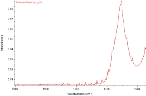
On this figure, the 1650 cm-1 band of water absorbs right in the amide I band of the protein. The only visible difference between the two spectrums is the absorption of amide II band at about 1550 cm-1.On this state, it’s not possible to work on that spectrum. To subtract the water of the protein spectrum, we must be careful to not subtract the protein itself. To avoid a too high subtraction of water, the water is subtracted with the width specific band of water between 1800 and 2400 cm-1. Figure 17 shows a subtraction of water on cytochrome C. The subtraction of water is controlled between 1750 and 2000 cm-1 by a flat base line.
19 3.2.2 Vapour correction
Not only liquid water absorb on the amide I band. Water vapour appears as well notably between 1600 and 1700 cm-1. Figure 18 shows the spectrum of a protein and the spectrum of vapour.
Figure 18: Red: Infrared spectrum of water vapours. Blue: Spectrum of cytochrome C after subtraction of water and vapour. Spectrums are on common scale
Vapour absorb right on the amide I band but also before and after. If it’s not possible to use the area at 1300 – 1600 cm-1, the area after 1700 cm-1 is free of any protein absorbance. To avoid any wrong subtraction due to the protein absorbance, area between 1750 and 1850 is used to check the subtraction.
Two peaks appear between 2200 and 2400 cm-1. These are peaks from carbon dioxide. Even if these peaks are independent of protein and liquid water, they can’t be used. After subtracting vapour on the important area, we can see that carbon dioxide is still appearing at 2350 cm-1.
To obtain a good subtraction, it’s necessary to focus on a peak that won’t disappear. Four points of a same peak are chosen. Such a peak is present between 1770 and 1775 cm-1. This peak is not possible to eliminate. It is either positive, negative or, when the subtraction is determine as optimal, has both a positive and negative part. Figure 19
20
Figure 19: Optimal vapour subtraction between 1750 and 1800 cm-1. Arrow: four wavelengths to check.
Both the first and last arrows are part of the base line and won’t move. The second arrow and the third arrow must be split around the base line. Even if it appears not to be a straight line, when looking the whole spectrum, the subtraction appears to be well done. Figure 20 shows the protein spectrum between 1300 and 1950 cm-1.
Figure 20: Spectrum of protein after water and vapour subtracting
On this spectrum, the area at 1770 cm-1, which is the one used to subtract vapour, is clearly background noise. By looking at the amide I and amide II area, the spectrum appears as clean even before the S-G smooth.
21 3.2.3 Smoothing
Smoothing is made by an S-G algorithm. To apply this algorithm, the number of points used by the smoothing must be set with high consequences on the final spectrum. Figure 21 shows the comparison between the same spectrums smoothed five times with different parameters.
Figure 21: Spectrum of Cytochrome C after 2nd derivative with different smoothing parameters. Blue: 5 points. Red: 7 points. Green: 9 points. Cyan: 11 points. Violet: 13 points
In this case, it’s quite easy to eliminate the 5 points smoothing. This one creates a high number of peaks without keeping a regular base line. Most of the attempt peaks are present, but some of them don’t appear while we’ve got some extra peaks. Due to the algorithm, the spectrum can be deformed by the smoothing procedure. So it’s really important to use the less invasive parameter to avoid modifying the final result by the mathematical process.
With a 13 points smoothing, some peaks disappeared, which modify the final result. But then, the three other smoothing parameter show similar spectrum. Only the 9 points S-G smooth is kept due to the presence of two distinctive peaks specific to β-sheet at 1691 and 1696 cm-1 and a better base line compared to the other smoothing. With a smaller number of points, the base line can’t be well defined and with a higher number of points, the peaks are too attenuated to identify the specific wavelength of the secondary structure.
22 3.2.4 S-G 2nd derivative
To analyse the smooth spectrum and get peaks to emerge, it is necessary to not stay on the base spectrum. Even if it’s possible to see some structure appearing as shoulder on the amide I band, it is not possible to determine any structure ratio. A curve fitting on a non-processed protein spectrum was tried without result. To have a usable curve fitting, it is necessary to have a Gaussian curve fitting to attribute every single Gaussian on a single secondary structure type and it is not possible to apply a curve fitting without using too much Gaussian to be pertinent. So a 2nd derivative of the spectrum is obtained by an S-G algorithm. Figure 22 shows a processed spectrum with different S-G 2nd derivative parameter.
Figure 22: 2nd derivative spectrum of cytochrome C with different S-G 2nd derivative parameter. Red: no derivative. Yellow: 3 points 2nd derivative. Blue: 5 points 2nd derivative. Purple: 7 points 2nd derivative.
Applying 2nd derivative make peaks appear relative to secondary structure motive. Using different parameter doesn’t change the global aspect of the spectrum. Each three derivative spectrum have the same peaks and integrate them, result on the same secondary structure ratio.
The difference is on the number of visible peaks. With a seven points derivative, there are eleven peaks on the 1600 – 1700 cm-1 area. Seventeen and twenty two for five point respectively three points derivative. Based on the work of Kong (Kong J., 2007), there are fourteen define peaks for secondary structure in amide I band. The five points have all the fourteen frequencies attribute to peaks of spectrum without too much parasite peaks. The five points derivative is then chosen for the data processing.
23 3.2.5 Fourier self-deconvolution
The Fourier self deconvolution method is based on the supposition that there are peaks specific to each secondary structure that occur at defined frequencies. The FSD deconvolutes the spectrum and, by the same token, make the peaks appear relative to the secondary structure motive. To avoid aberration, it is necessary to not force some extreme deconvolution’s parameters. The two modifiable parameters are the bandwidth and enhancement.
By modifying the bandwidth, the width of each peak will be reduced or increased and by modifying the enhancement, peaks will be more or less defined. Based on the work of Byler and Susi (Byler D.M., 1986), chosen parameters are the standard one, a bandwidth of 13 and an enhancement of 2.4. Others parameter had been tried but by making changes to these parameter, most of the time, aberration —like impossible base line definition due to negative peak— occur on the final spectrum. The final spectrum is curve-fitted with Gaussian and each Gaussians are integrated and attributed to a secondary structure.
Figure 23 shows an example of the deconvoluted and curve fitted spectrum of myoglobin.
Figure 23: Deconvoluted spectrum of myoglobin with curve fitting. Blue points: deconvoluted spectrum. Red: curve fitting. Cyan: gaussians attributed to beta sheets. Red: gaussians attributed to alpha helix. Yellow: Gaussians attributed to beta turn.
24
3.3
Final method
The final method had the following FTIR parameters:
o Concentration: 5 % w/V in water
o Pathlength: 6 μm CaF2 cell
o Number of scans: 100
o Resolution: 2 cm-1
o Aperture: 30
o Range: 4000-400 cm-1
Data processing:
o Subtraction of water: straight line between 1600 and 1700 cm-1
o Subtraction of vapour: minimal peak between 1765 and 1775 cm-1
o Smoothing: nine points Savitsky-Golay algorithm
o Derivative: five points Savitsky-Golay derivative
o Integration: using a MATLAB script
25
4
Results
Results are obtained for ten different protein using two different methods and compared to reference. The two used methods are the ones describe previously. The Fourier self-deconvolution method was applied using the following parameters. A bandwidth of 13 cm-1 and an enhancement of 2.3 based on the work of Byler and Susi (Byler D.M., 1986).
Integration of processed spectrum with smoothing and S-G 2nd derivate was made without considering each band separately. Only the global area of sheet band, α-helix band and β-turn band are measured. Figure 24 shows an example of integration area for cytochrome C with 2nd derivative analysis.
Figure 24: Integration of 2nd derivative inverted spectrum of cytochrome C. Green: beta-sheet. Blue: random coil. Red: alpha-helix. Cyan: beta-turn
Based on the work of Kong (Kong J., 2007), an assignment of secondary structure on the peaks of the spectrum is made. Peaks can experience a small switch of about ± 4 cm-1 and sometimes more.
On Table 2, all the frequency and assignment for secondary structure are listed for the amide I band, the area between 1600 and 1700 cm-1.
26
Table 2: frequency and assignment of peaks and secondary structure on amide I band.
frequency assignment 1624 β-sheet 1627 β-sheet 1633 β-sheet 1638 β-sheet 1642 β-sheet 1648 Random coil 1656 α-helix 1663 310-helix 1667 β-turn 1675 β-turn 1680 β-turn 1685 β-turn 1691 β-sheet 1696 β-sheet
Three peaks are visible on α-helix instead of the two attempt peaks. For β-turn, six peaks appear instead of four. The choice has been made to not integrate every single peak separately but to integrate the area containing the desired structure.
Results for ten proteins are obtaind using both the 2nd derivative and Fourier self-deconvolution method and compared to two X-Ray references and one IR Reference. Table 3 lists all of the results and references.
27
Table 3: Composition of protein secondary structure determined by IR with S-G 2nd derivate and Fourier self-deconvolution
Protein Secondary Structure Method α-helix β-Sheet turn random
Lysozyme 40 24 27 9 2nd derivative 38 22 28 12 Fsd 42 6 23 29 X-Ray (a) 45 19 23 13 X-Ray (b) 40 19 27 14 IR (c) Hemoglobin 57 20 23 0 2nd derivative 48 25 27 0 Fsd 77 0 9 14 X-Ray (a) 87 0 7 6 X-Ray (b) 78 12 10 0 IR (c) Myoglobin 66 25 9 0 2nd derivative 59 18 23 0 Fsd 74 0 13 13 X-Ray (a) 85 0 8 7 X-Ray (b) 85 7 8 0 IR (c) Cytochrome C 42 21 23 14 2nd derivative 45 16 25 14 Fsd 41 0 17 41 X-Ray (a) 48 10 17 25 X-Ray (b) 42 21 25 12 IR (c) α-Chymotrypsin 6 47 36 11 2nd derivative 7 44 31 18 Fsd 8 50 27 15 X-Ray (b) 9 47 30 14 IR (c) Trypsin 24 43 25 8 2nd derivative 15 38 30 17 Fsd 9 56 24 11 X-Ray (b) 9 44 38 9 IR (c) RNase A 10 55 33 2 2nd derivative 13 42 36 9 Fsd 21 33 15 32 X-Ray (a) 23 46 21 10 X-Ray (b) 15 40 36 9 IR (c) Concavanaline A 13 51 29 20 2nd derivative 7 56 27 10 Fsd 4 45 11 41 X-Ray (a) 3 60 22 15 X-Ray (b) 8 58 26 8 IR (c) IgG 5 52 33 10 2 nd derivative 12 50 30 8 Fsd
28 7 50 14 29 X-Ray (a) 3 67 18 12 X-Ray (b) 3 64 28 5 IR (c) Pepsin 18 52 22 8 2nd derivative 12 47 19 12 Fsd 15 44 14 28 X-Ray (a)
(a) SwissProt/UniProt : http://www.uniprot.org/uniprot/?query=reviewed%3Ayes (b) Levitt and Greer (Levitt M., 1977)
(c) Dong, Huang and Caughey (Dong A., 1990)
Results for most proteins are in the same proportion than X-Ray references. That confirms the validity of the analysis. Looking further, there is a big difference, about 20 % in some cases for secondary structure determination. The Fourier self-deconvolution method shows results similar to 2nd derivate one.
Figure 25 amply demonstrates all the similarities of the two methods. All the most important spectrum are visible on both method and even on the non-processed spectrum.
Figure 25: comparison between non processed spectrum, 2nd derivative one and deconvoluted one. Green: non processed spectrum. Blue: self deconvoluted spectrum. Red: 2nd derivative spectrum.
29
5
Discussion
5.1
Water and vapour subtraction
Most publications (Dong A., 1990) (Kong J., 2007) used a visual check to approve the subtraction. Due to the randomness of such a process because of a high subjective evaluation, the choice of an automatic subtraction based on defined parameter make a good method to suppress this subjective part. By using this automatic subtraction on a MATLAB script, we obtain good results on all the tested protein with the possibility of making a manual control at all the steps of the processing to avoid aberrations that can occur, like a wrong ratio because the concrete one is out of the tested range.
The water is still subtracting base on the area between 1750 and 2000. But, only three points are used and we search the subtraction ratio that made these three points on a straight line. This mean calculating the linear regression of these wavelengths after subtraction for all ratios and keeping the one with the best correlating coefficient. The chosen wavelength mustn’t be on a peak of the vapour spectrum and they must be split on all the length but with these two conditions, any point can be used with the same result at the end. For certain protein, pepsin for example, we can observe an absorbance between 1700 and 1780. If one of the used points is in this area, the subtraction can be well done for most protein but will be completely aberrant in the case of the pepsin. To avoid complication due to this effect, the wavelengths used for the subtraction must be chosen out of this area.
5.2
Vapour subtraction
Vapour subtraction is an important part of the analysis. As for the water, vapour absorbs on the amide I area. This problem is that even with a purge or a higher resolution and number of scan of the spectrum, it is not possible to obtain a straight base line after subtraction. Figure 26 shows the problem of the subtraction. When subtracting the vapour, when one peak is correctly subtracted, another isn’t.
Figure 26: subtraction of vapour of a protein spectrum. (a) Optimal subtraction. (b) vapour excessively subtracted. (c) vapour insufficiently subtracted
30
Parameters used for the subtraction are subjectively chosen and give good results on all tested protein. By changing the method or processing, the subtraction of vapour must be redefined. A high ratio of one secondary structure can create a shoulder on the peak that can be seen as a peak from vapour. Due to this effect, it’s important to subtract vapour without looking between 1600 and 1700 cm-1. Particularly when making a manual subtraction that is made by the operator only.
5.3
Results
Results on proteins containing high ration of α-helix need a different integration due to a distortion of the environment around the alpha helix peak. Figure 27 shows the integration of the spectrum of haemoglobin.
Figure 27: Integration of 2nd derivative spectrum of haemoglobin
The base line for integration of alpha helix had to be change to fit better to the model. The used integration method place the base line to the lowest side-peak of the alpha-helix one. A constantly underestimate proportion of alpha helix is obtained for proteins with more than 60 % of alpha helix with both method.
31
To compare the result to the references, it is necessary to compare references with each other. It is normal to get some difference between IR and X-Ray (Kumosinski T. F., 1996). The two methods don’t work in the same way and there are different methods to do the IR determination. But even between two completely different methods, the proportions are the same and the result can be determined as similar. But even with the same method, when comparing the two X-Ray references, there are huge differences. Reference (a) is the more recent one. The bigger difference is the recurrent higher ratio of random coil on the reference (a). This high ratio of random coil has an impact on the three other structures.
The two methods show good result but none of them can be determine as better, only by looking with result. To determine which one is the best, we must know what the objective of this analysis is. If the objective is to know precisely the right secondary structure ratio, this method isn’t the good one. But if the objective is to know, with a relative precision and by knowing that the result isn’t the truth but depend on the used determination method, then this method works. On the same way, analysis of protein folding can easily be done with this method.
6
Conclusion and outlook
The development of an analytical method to quantify the secondary structure motives of a protein permitted to understand better the mechanism of secondary structure determination by FTIR. By analysing ten model proteins, the results obtained and compared to the one published by other people, had to be looked with an open mind. Most of result can’t really get compared with the work of someone else due to the difference between the method and method parameters. To get a global idea of a protein structure, such comparison can be made, but to get a more precise one, the only way is to use the same method.
Getting the secondary structure motives proportion with such an easy method like FTIR is a great thing, it allows with low cost an easy and fast analysis. By obtaining the secondary structure, it is now possible to analysis the refolding of a denatured protein or of one obtains from synthesis. More investigation should be done in the analysis of unfold protein and compared to fold one to confirm the validity of the method in these case.
32
7
Bibliography
Alberts B., J. A. (2002). Molecular Biology of the Cell. 4th edition. New York: Garland Science.
Barth, A. (2007). Infrared spectroscopy of proteins. Biochimica et Biophysica Acta (1767) , 1073-1101.
Byler D.M., S. H. (1986). Examination of the secondary sstructure of proteins by deconvoluted FTIR spectra. Biopolymers (25) , 469-487.
Dong A., H. P. (1990). Protein Secondary Structures in Water from Second-Derivative Amide I Infrared Spectra. Biochemistry (29) , 3303-3308.
Kabsch W., S. C. (1983). Dictionary of protein secondary structure: pattern recognition of hydrogen-bonded and geometrical features. Biopolymers (22) , 2577-2637.
Kong J., Y. S. (2007). Fourier Transform Infrared Spectroscopic Analysis of Protein Secondary Structures. Acta Biochimica et Biophysica Sinica (39) , 549-559.
Kumosinski T. F., U. J. (1996). Quantification of the global secondary structure of globular proteins by FTIR spectroscopy: comparison with X-ray crystallographic structure. Talanta
(43) , 199-219.
Levitt M., G. J. (1977). Automatic Identification of Secondary Structure in Globular Proteins.
Journal of Molecular Biology (114) , 181-239.
Pelton J. T., M. L. (2000). Spectroscopic Methods for Analysis of Protein Secondary Structure.
Analytical Biochemistry (277) , 167-176.
8
Annexe
1 Standard Operative Procedure: Analyse de la structure secondaire de protein (in French)
2 MATLAB script of SOP
Annexe 1 : SOP
HES–SO Valais
Analyse de la structure
secondaire de protéine Version 1 Domaine d’application : CA
1.
Domaine d’application
Détermination des ratios des différentes structures secondaire présentes d’une protéine en solution aqueuse à 5% m/v soit 50 mg/ml.
2.
Mesure de précaution
Précautions standards lors de l’utilisation de produits chimiques. Les précautions à respecter en cours d’analyse sont citées au fil de ce mode opératoire.
3.
Principe de détermination
Analyse de structure secondaire par Infrarouge à transformée de Fourier (FTIR) suivi d’un traitement de donnée sur MATLAB.
4.
Appareillage et produits
4.1.
Appareillage
o FTIR o Spacer 6 μm o OMNIC o MATLAB4.2.
Produits
o Azote 4.5 o Eau MilliQ5.
Préparation des échantillons, paramètre de mesure
5.1.
Préparation de la référence de l’eau
25 μl d’eau MilliQ sont introduits directement dans le trou de la cellule. Au moyen d’une seringue remplie d’air, poussé l’échantillon jusqu’à ce que le liquide remplisse la totalité du volume du spacer.
5.2.
Référence de la vapeur d’eau
L’analyse de la vapeur d’eau se fait sans cellule de mesure, avec l’air ambiant comme échantillon.
5.3.
Préparation des échantillons à analysé
Dans un eppendorf de 1.5ml, transférer successivement 1.25mg de protéine à analyser et 25 μl d’eau MilliQ. Agiter puis centrifuger 3 secondes. Répéter éventuellement la manœuvre si la protéine à mal été solubilisée.
25 μl de l’échantillon sont introduits directement dans le trou de la cellule. Au moyen d’une seringue remplie d’air, poussé l’échantillon jusqu’à ce que le liquide remplisse la totalité du volume du spacer.
Annexe 1 : SOP
HES–SO Valais
Analyse de la structure
secondaire de protéine Version 1 Domaine d’application : CA
5.4.
Mesure du background
Le background est mesuré sans cellule de mesure avec une purge de 2 bars maintenu durant 10 minutes avant l’analyse et conservée durant toute la durée de l’analyse.
5.5.
Analyse
L’analyse de l’eau et de la vapeur d’eau ne doit pas être effectuée à chaque fois.
Pour l’analyse de protéine et de la référence de l’eau, introduire la cellule de mesure dans l’appareil, fermer l’appareil, fixer la pression de sortie de l’azote à 2 bars. Purger durant 10 minutes. En conservant le débit d’azote, collecter l’échantillon en sélectionnant « Collect Sample » sous l’onglet « Collect ».
Pour l’analyse de la vapeur d’eau, sans introduire la cellule de mesure et sans purge d’azote, collecter le spectre de mesure de la même manière que cité précédemment.
5.6.
Paramètre de mesure
• Collect
o Nombre de scans : 100
o Résolution : 2
o Format Final : SingleBeam
o Correction : aucune
o Save interferograms
o Aperture : 30
o Range : 4000-400 cm-1
6.
Traitement des données
6.1.
Spectres de références
Les spectres de références de l’eau (Water), de la vapeur d’eau (Vapor) et du background (background) sont présent sous :
C:\Users\f103\Documents\OMNIC\Spectra\Protein_folding\reference
6.2.
Traitement du spectre de la protéine par OMNIC
Les étapes du traitement des spectres sont effectuées en absorbance. Les spectres initiaux sont reprocessé en absorbance avec le spectre Background.spa comme background. Le chemin logique pour effectuer la manipulation est le suivant :
Process > Reprocess > Séléctionner «Absorbance» > Choisir le Background > OK
Annexe 1 : SOP
HES–SO Valais
Analyse de la structure
secondaire de protéine Version 1 Domaine d’application : CA
6.3.
Traitement par MATLAB
Déplacer le spectre à analyser dans le répertoire MATLAB C:\Users\f103\Documents\MATLAB. Lancer l’application MATLAB grâce au raccourci présent sur le bureau ou en cliquant sur matlab.exe dans C:\Program Files\MATLAB\R2010a\bin\. Vérifier que votre spectre apparaît dans la fenêtre «Current Folder» située à gauche dans MATLAB. Si la fenêtre «Current Folder» n’est pas visible, Sélectionner «Current Folder» sous l’onglet «Desktop» de la barre de raccourci MATLAB.
Pour effectuer l’analyse du spectre voulu, entré dans la fenêtre «Command Window» la fonction suivante :
Prot_Struct_sec(‘Spectre à analyser’,’spectre de l’eau’,’spectre de la vapeur d’eau’)
MATLAB affichera après quelques secondes de calcule la fraction de β-turn sous frac_turn, la fraction d’α-hélice sous frac_ahelice et la fraction de β-sheet sous frac_bsheet_tot. La figure 4 montre un exemple avec le spectre du Cytochrome C (nommé Cyt_C_nt.spc). 5 spectres sont également générés pour permettre le contrôle des différentes étapes de l’analyse. Les paramètres d’acceptation sont décrits dans les chapitres 6.2 à 6.5. La figure 5 montre ces 5 spectres générés par l’analyse du cytochrome C.
Annexe 1 : SOP
HES–SO Valais
Analyse de la structure
secondaire de protéine Version 1 Domaine d’application : CA
Figure 2: Spectre générés par l'analyse MATLAB. Figure 1°: résultat de la soustraction de l'eau. Figure 2 : résultat de la soustraction de la vapeur d’eau. Figure 3 : résultat de l’affinage du spectre. Figure 4 : 2ème dérivée du spectre. Figure 5 : Découpage de l’intégration du spectre final.
6.4.
Soustraction du signal de l’eau
La soustraction est contrôlée dans la zone de 1750 à 2000 cm-1. Cette zone doit apparaître comme plate pour confirmer que la soustraction a eu lieu correctement. Si la soustraction n’est pas réalisée correctement, elle doit être effectuée manuellement sur le logiciel OMNIC. Pour effectuer la soustraction, sélectionner le spectre de la protéine puis le spectre de l’eau ouvert dans la même fenêtre. Sélectionner «soustraire» dans l’onglet «Process» ou utiliser le raccourci « CTRL + U ».
Modifier le facteur de soustraction avec la molette (figure 3, A) et sélectionner l’intervalle 1650 – 2000 à l’aide de l’outil de sélection (figure 3, B). Modifier le facteur jusqu’à une soustraction correcte (figure 4).
Annexe 1 : SOP
HES–SO Valais
Analyse de la structure
secondaire de protéine Version 1 Domaine d’application : CA
Figure 3 : Soustraction de l’eau du spectre du cytochrome C. A : molette du facteur de soustraction, B : intervalle de sélection.
Annexe 1 : SOP
HES–SO Valais
Analyse de la structure
secondaire de protéine Version 1 Domaine d’application : CA
6.5.
Soustraction du signal de la vapeur d’eau
La soustraction de la vapeur d’eau est considérée comme correcte lorsque le signal du à la vapeur d’eau est le plus petit possible. A partir du spectre dont l’eau à été soustraite, soustraire la vapeur d’eau en suivant la même procédure que pour l’eau dans l’intervalle 1750-1850. Lorsque la ligne de base est la plus plate possible, la soustraction est considérée comme bonne. La figure 5 montre la soustraction du cytochrome C.
Figure 5: soustraction de la vapeur d'eau du cytochrome C.
6.6.
Génération de la 2
èmedérivée du spectre
Le spectre de la protéine est maintenant affiné en utilisant un «smooth» de Savitzky-Golay à 9 point. Sélectionner «smooth» dans l’onglet «Process», puis, dans le menu déroulant, sélectionner «9» et appuyer sur OK.
La deuxième dérivée est obtenue selon l’algorithme de Savitzky-Golay à 5 point. Sélectionner «Derivative» dans l’onglet «Process». Sélectionner «Derivative Second» cocher la case «Savitzky-Golay» et sélectionner «5 point» et «Polynomial order 3». La figure 6 montre la fenêtre de derivée du programme OMNIC.
Annexe 1 : SOP
HES–SO Valais
Analyse de la structure
secondaire de protéine Version 1 Domaine d’application : CA
Figure 6: Fenêtre de dérivée du logiciel OMNIC.
6.7.
Calcul des ratios de structures secondaires par MATLAB.
Sauvegarder le spectre de la deuxième dérivée au format .spc. La structure secondaire est calculée en utilisant le scripte Manual_area() avec les six longueur d’onde de la plus petite à la plus grande dans MATLAB.
Pour utiliser le script, introduire dans la fenêtre «Command Window»
Par exemple :
Manual_area(‘Spectre à analyser’,1621,1643,1649,1666,1692,1699)
MATLAB affichera après quelques secondes de calcule la fraction de β-turn sous frac_turn, la fraction d’α-hélice sous frac_ahelice et la fraction de β-sheet sous frac_bsheet_tot.
7.
Modification de l’intégration
L’intégration de la deuxième dérivée peut mal se faire du à un léger décalage de certain pic. Dans le cas d’une intégration dont certain pic ne sont pas pris en compte alors qu’ils le devraient ou sont pris en compte alors qu’ils ne le devraient pas, il est possible de modifier les intervalles d’intégration en utilisant Manual_Prot() avec les six longueur d’onde de la plus petite à la plus grande.
Pour le cytochrome C :
Annexe 1 : SOP
HES–SO Valais
Analyse de la structure
secondaire de protéine Version 1 Domaine d’application : CA
8.
Pics spécifiques aux différentes structures secondaires
Le tableau 1 montre les différents pics spécifiques aux différentes structures secondaires ainsi que leurs longueurs d’onde.
Tableau 1: fréquences et assignement des structures secondaires dans la bande amide I
fréquence assignement 1624 β-feuillet 1627 β-feuillet 1633 β-feuillet 1638 β-feuillet 1642 β-feuillet 1648 Bobine aléatoire 1656 α-hélice 1663 310-hélice 1667 β-turn 1675 β-turn 1680 β-turn 1685 β-turn 1691 β-feuillet 1696 β-feuillet
Annexe 2 : Code MATLAB
1Script « Prot_Struct_sec() »
function Prot_Struct_sec(f,g,h) close all W1=2070; W2=2193; W3=2318; V1=2317; V2=2312; V3=2310; V4=2305; f1='.spc'; f2='_sub'; f3='.xls'; f4=[f f1]; f5=[f f3]; f6=[f f2 f3]; g1=[g f1]; h1=[h f1]; spec_1=tgspcread(f4); spec_2=tgspcread(g1); spec_3=tgspcread(h1); %xlswrite(f5,[spec_1.X,spec_1.Y]); spec_l=substract_Water(spec_1, spec_2,W1,W2,W3); spec_m=substract_Vapor(spec_l, spec_3,V1,V2,V3,V4); %xlswrite(f6,[spec_m.X,spec_m.Y]); %%%%%%%%%%%%%%%%%%%%%%%%%%%%% %contrôle de la soustraction% %%%%%%%%%%%%%%%%%%%%%%%%%%%%% figure hold on plot(spec_l.X,spec_l.Y);title('substract Water');
figure;
hold on
plot(spec_m.X,spec_m.Y);
title('substract Vapor');
spec_n.Y=smooth(spec_m.Y,9,'sgolay',3); spec_n.X=spec_m.X; figure; hold on plot(spec_n.X,spec_n.Y);
title('smoothed spectrum');
%%%%%%%%% %2nd derivative %%%%%%%%% N = 3; F = 5; [b,g] = sgolay(N,F); dx = 1; HalfWin = ((F+1)/2) -1; for n = (F+1)/2:2997-(F+1)/2, % 2nd differential
Annexe 2 : Code MATLAB
2
SG2(n) = 2*dot(g(:,3)', spec_n.Y(n - HalfWin: n + HalfWin))';
end SG2 = SG2/(dx*dx); figure; hold on plot(spec_n.X(1:2994),SG2);
title('2nd derivative spectrum');
hold off %%%%%%%%%%%%%%%%%%%%%% %4th derivative %%%%%%%%%%%%%%%%%%%%%% HalfWin = ((F+1)/2) -1; for n = (F+1)/2:2994-(F+1)/2,
SG4(n) = 2*dot(g(:,3)', SG2(n - HalfWin: n + HalfWin))';
end SG4 = SG4/(dx*dx); SG4_2.X=spec_n.X(2390:2500); SG4_2.Y=SG4(2390:2500)'; figure; hold on plot(SG4_2.X,SG4_2.Y); [pks,locs]=findpeaks(SG4_2.Y); %%%%%%%%%%%%%%%%%%%%%% %paramètre d'integration %%%%%%%%%%%%%%%%%%%%%% [r,WL3]=find(SG4==min(SG4(2435:2441))); [r,WL1]=find(SG4==min(SG4(2465:2471))); [r,WL2]=find(SG4==min(SG4(2442:2448))); [r,WL4]=find(SG4==min(SG4(2419:2426))); [r,WL5]=find(SG4==min(SG4(2392:2397))); [r,WL6]=find(SG4==min(SG4(2382:2390))); areabast(SG2,spec_m,WL1,WL2,WL3,WL4,WL5,WL6) end
function [spec_f]=substract_Water(spec_1, spec_2, W1, W2, W3)%, W4, W5) fact_W=0;
rmax=0;
%%%%%%%%%%%%%%%%%%%%%%%%%%%%%%%%%%%%%%%%%%%%%%%%%%%%%%%%%%%%% %boucle "for" dont on fait varier le facteur de soustraction% %du spectre de la protéine par le spectre de l'eau%%%%%%%%%%% %%%%%%%%%%%%%%%%%%%%%%%%%%%%%%%%%%%%%%%%%%%%%%%%%%%%%%%%%%%%% for i=0.5:0.0001:1.5 t1=spec_1.Y(W1)-i*spec_2.Y(W1); t2=spec_1.Y(W2)-i*spec_2.Y(W2); t3=spec_1.Y(W3)-i*spec_2.Y(W3);
x=[spec_1.X(W1) spec_1.X(W2) spec_1.X(W3)]; y=[t1 t2 t3]; c=corrcoef(x,y); r=c(1,2)^2; %%%%%%%%%%%%%%%%%%%%%%%%%%%%%%%%%%%%%%%%%%%%%%%%%%%%%%%%%%%%%%%% %lorsque le coefficient de correlation est le plus proche de 1,% %la zone où l'eau liquide absorbe a été soustraite au maximum%%%
%%%%%%%%%%%%%%%%%%%%%%%%%%%%%%%%%%%%%%%%%%%%%%%%%%%%%%%%%%%%%%%% if (r>rmax) fact_W=i; rmax=r; end end spec_f.X=spec_1.X; spec_f.Y=spec_1.Y-fact_W*spec_2.Y;
Annexe 2 : Code MATLAB
3
%%%%%%%%%%%%%%%%%%%%%%%%%%%%%%%%%%%%%%%%%%%%%%%%%%%%%%%%%%%%%%%%%%%%%%%%%%%%%%%%%%%%% %une fois le facteur de soustraction déterminé, la totalité du spectre est soustrait% %%%%%%%%%%%%%%%%%%%%%%%%%%%%%%%%%%%%%%%%%%%%%%%%%%%%%%%%%%%%%%%%%%%%%%%%%%%%%%%%%%%%%
fact_W
end
function [spec_g]=substract_Vapor(spec_f, spec_3, V1, V2, V3, V4) fact_V=0; rmax=0; for i=-0.3:0.0001:0.3 t1=spec_f.Y(V1)-i*spec_3.Y(V1); t2=spec_f.Y(V2)-i*spec_3.Y(V2); t3=spec_f.Y(V3)-i*spec_3.Y(V3); t4=spec_f.Y(V4)-i*spec_3.Y(V4);
x=[spec_f.X(V1) spec_f.X(V2) spec_f.X(V3) spec_f.X(V4)]; y=[t1 t2 t3 t4]; c=corrcoef(x,y); r=c(1,2)^2; if (r>rmax) fact_V=i; rmax=r; end end spec_g.X=spec_f.X; spec_g.Y=spec_f.Y-fact_V*spec_3.Y; fact_V end function areabast(SG2,spec_m,WL1,WL2,WL3,WL4,WL5,WL6)%wavelength_1,wavelength_2 turn_2=WL4; turn_1=WL5; alpha_1=WL3; beta_2=WL1; beta_1=WL2; beta_3=WL6; spec.X=[spec_m.X(WL6:WL1)]'; spec.Y=[SG2(WL6:WL1)]'; %Base ligne poly_x=[spec.X(WL1-WL6+1) spec.X(WL6-WL6+1)]; poly_y=[spec.Y(WL1-WL6+1) spec.Y(WL6-WL6+1)]; p=polyfit(poly_x,poly_y,1); BL=spec.X*p(1)+p(2); BLa=BL; %substract spec_f.X=spec.X; spec_f.Y=(spec.Y-BL')*(-1); spec_f_a.Y=(spec.Y-BLa')*(-1); %area_curve ahelice=trapz(spec_f.X(turn_2-beta_3+1:alpha_1-beta_3+1),spec_f.Y(turn_2-beta_3+1:alpha_1-beta_3+1)); tot=trapz(spec_f.X,spec_f.Y)-ahelice; turn=trapz(spec_f.X(turn_1-beta_3+1:turn_2-beta_3+1),spec_f.Y(turn_1-beta_3+1:turn_2-beta_3+1)); %if BLa>BL % ahelice=trapz(spec_f.X(turn_2-beta_3+1:alpha_1-beta_3+1),spec_f_a.Y(turn_2-beta_3+1:beta_1-beta_3+1)); % tot=tot+ahelice; %else ahelice=trapz(spec_f.X(turn_2-beta_3+1:alpha_1-beta_3+1),spec_f.Y(turn_2-beta_3+1:alpha_1-beta_3+1)); tot=tot+ahelice; %end bsheet=trapz(spec_f.X(beta_1-beta_3+1:beta_2-beta_3+1),spec_f.Y(beta_1-beta_3+1:beta_2-beta_3+1));
Annexe 2 : Code MATLAB
4 bsheet_2=trapz(spec_f.X(1:turn_1-beta_3+1),spec_f.Y(1:turn_1-beta_3+1)); figure hold on plot(spec_f.X(turn_1-beta_3+1:turn_2-beta_3+1),spec_f.Y(turn_1-beta_3+1:turn_2-beta_3+1),'Color','c') %figure %if BLa>BL % plot(spec_2.X(turn_2-beta_3+1:beta_1-beta_3+1),spec_f.Y(turn_2-beta_3+1:beta_1-beta_3+1),'Color','r') %else plot(spec_f.X(turn_2-beta_3+1:alpha_1-beta_3+1),spec_f.Y(turn_2-beta_3+1:alpha_1-beta_3+1),'Color','r') %end plot(spec_f.X(alpha_1-beta_3+1:beta_1-beta_3+1),spec_f.Y(alpha_1-beta_3+1:beta_1-beta_3+1),'Color','b') plot(spec_f.X(beta_1-beta_3+1:beta_2-beta_3+1),spec_f.Y(beta_1-beta_3+1:beta_2-beta_3+1),'Color','g') plot(spec_f.X(1:turn_1-beta_3+1),spec_f.Y(1:turn_1-beta_3+1),'Color','g')plot(spec_f.X(1:beta_2-beta_3+1),0,'Color','black')
frac_turn=turn/tot*100 frac_ahelice=ahelice/tot*100 frac_bsheet=bsheet/tot*100; frac_bsheet_2=bsheet_2/tot*100; frac_bsheet_tot=frac_bsheet+frac_bsheet_2 t100=frac_turn+frac_ahelice+frac_bsheet_tot; end
Script « Manual_Prot »
function Manual_Prot(f,g,h,wave1,wave2,wave3,wave4,wave5,wave6) WL1=round(-1.0371*wave1+4149); WL2=round(-1.0371*wave2+4149); WL3=round(-1.0371*wave3+4149); WL4=round(-1.0371*wave4+4149); WL5=round(-1.0371*wave5+4149); WL6=round(-1.0371*wave6+4149); close all W1=2203; W2=2277; W3=2358; V1=2317; V2=2312; V3=2310; V4=2305; %%%%%%%%%%%%%%%%%%%%%%%%%%%%%%%%%%%%%%%%%%%%%%%%%%%%%%%% %chargement des spectres de protéine, eau, vapeur d'eau% %%%%%%%%%%%%%%%%%%%%%%%%%%%%%%%%%%%%%%%%%%%%%%%%%%%%%%%% f1='.spc'; f2='_sub'; f3='.xls'; f4=[f f1]; f5=[f f3]; f6=[f f2 f3]; g1=[g f1]; h1=[h f1]; spec_1=tgspcread(f4); spec_2=tgspcread(g1); spec_3=tgspcread(h1); %xlswrite(f5,[spec_1.X,spec_1.Y]); spec_l=substract_Water(spec_1, spec_2,W1,W2,W3);Annexe 2 : Code MATLAB
5 spec_m=substract_Vapor(spec_l, spec_3,V1,V2,V3,V4); %xlswrite(f6,[spec_m.X,spec_m.Y]); %%%%%%%%%%%%%%%%%%%%%%%%%%%%% %contrôle de la soustraction% %%%%%%%%%%%%%%%%%%%%%%%%%%%%% figure hold on plot(spec_l.X,spec_l.Y);title('substract Water');
figure;
hold on
plot(spec_m.X,spec_m.Y);
title('substract Vapor');
spec_n.Y=smooth(spec_m.Y,9,'sgolay',3); spec_n.X=spec_m.X; figure; hold on plot(spec_n.X,spec_n.Y);
title('smoothed spectrum');
%%%%%%%%% %2nd derivative %%%%%%%%% N = 3; F = 5; [b,g] = sgolay(N,F); dx = 1; HalfWin = ((F+1)/2) -1; for n = (F+1)/2:2997-(F+1)/2,
SG2(n) = 2*dot(g(:,3)', spec_n.Y(n - HalfWin: n + HalfWin))';
end SG2 = SG2/(dx*dx); figure; hold on plot(spec_n.X(1:2994),SG2);
title('2nd derivative spectrum');
hold off %%%%%%%%%%%%%%%%%%%%%% %4th derivative %%%%%%%%%%%%%%%%%%%%%% HalfWin = ((F+1)/2) -1; for n = (F+1)/2:2994-(F+1)/2,
SG4(n) = 2*dot(g(:,3)', SG2(n - HalfWin: n + HalfWin))';
end SG4 = SG4/(dx*dx); SG4_2.X=spec_n.X(2390:2500); SG4_2.Y=SG4(2390:2500)'; areabast(SG2,spec_m,WL1,WL2,WL3,WL4,WL5,WL6) end
function [spec_f]=substract_Water(spec_1, spec_2, W1, W2, W3)%, W4, W5) fact_W=0;
rmax=0;
%%%%%%%%%%%%%%%%%%%%%%%%%%%%%%%%%%%%%%%%%%%%%%%%%%%%%%%%%%%%% %boucle "for" dont on fait varier le facteur de soustraction% %du spectre de la protéine par le spectre de l'eau%%%%%%%%%%% %%%%%%%%%%%%%%%%%%%%%%%%%%%%%%%%%%%%%%%%%%%%%%%%%%%%%%%%%%%%%
for i=0.5:0.0001:1.5
Annexe 2 : Code MATLAB
6
t2=spec_1.Y(W2)-i*spec_2.Y(W2); t3=spec_1.Y(W3)-i*spec_2.Y(W3);
x=[spec_1.X(W1) spec_1.X(W2) spec_1.X(W3)]; y=[t1 t2 t3]; c=corrcoef(x,y); r=c(1,2)^2; %%%%%%%%%%%%%%%%%%%%%%%%%%%%%%%%%%%%%%%%%%%%%%%%%%%%%%%%%%%%%%%% %lorsque le coefficient de correlation est le plus proche de 1,% %la zone où l'eau liquide absorbe a été soustraite au maximum%%%
%%%%%%%%%%%%%%%%%%%%%%%%%%%%%%%%%%%%%%%%%%%%%%%%%%%%%%%%%%%%%%%% if (r>rmax) fact_W=i; rmax=r; end end spec_f.X=spec_1.X; spec_f.Y=spec_1.Y-fact_W*spec_2.Y; %%%%%%%%%%%%%%%%%%%%%%%%%%%%%%%%%%%%%%%%%%%%%%%%%%%%%%%%%%%%%%%%%%%%%%%%%%%%%%%%%%%%% %une fois le facteur de soustraction déterminé, la totalité du spectre est soustrait% %%%%%%%%%%%%%%%%%%%%%%%%%%%%%%%%%%%%%%%%%%%%%%%%%%%%%%%%%%%%%%%%%%%%%%%%%%%%%%%%%%%%%
fact_W
end
function [spec_g]=substract_Vapor(spec_f, spec_3, V1, V2, V3, V4) fact_V=0; rmax=0; for i=-0.3:0.0001:0.3 t1=spec_f.Y(V1)-i*spec_3.Y(V1); t2=spec_f.Y(V2)-i*spec_3.Y(V2); t3=spec_f.Y(V3)-i*spec_3.Y(V3); t4=spec_f.Y(V4)-i*spec_3.Y(V4);
x=[spec_f.X(V1) spec_f.X(V2) spec_f.X(V3) spec_f.X(V4)]; y=[t1 t2 t3 t4]; c=corrcoef(x,y); r=c(1,2)^2; if (r>rmax) fact_V=i; rmax=r; end end spec_g.X=spec_f.X; spec_g.Y=spec_f.Y-fact_V*spec_3.Y; fact_V end function areabast(spec_1,spec_2,wavelength_3,wavelength_4,wavelength_5,wavelength_6,wavelength_7,wavele ngth_8)%wavelength_1,wavelength_2 turn_2=wavelength_6; turn_1=wavelength_7; alpha_1=wavelength_5; beta_2=wavelength_3; beta_1=wavelength_4; beta_3=wavelength_8; spec.X=[spec_2.X(wavelength_8:wavelength_3)]'; spec.Y=[spec_1(wavelength_8:wavelength_3)]'; %Base ligne %BL=mean(max(spec_1(2382:2389),max(spec_1(2453:2485)))); poly_x=[spec.X(wavelength_3-wavelength_8+1) spec.X(wavelength_8-wavelength_8+1)];%[spec.X(wavelength_8-wavelength_8+1) spec_1.X(wavelength_3-wavelength_8+1)] poly_y=[spec.Y(wavelength_3-wavelength_8+1) spec.Y(wavelength_8-wavelength_8+1)];%[spec.Y(wavelength_8-wavelength_8+1) spec_1.Y(wavelength_3-wavelength_8+1)] p=polyfit(poly_x,poly_y,1); BL=spec.X*p(1)+p(2);
Annexe 2 : Code MATLAB
7
%if 1.5*max(max(spec_1(2385:2389),max(spec_1(2453:2479)))) < max(spec_1(2422:2441)) % BLa=max(spec_1(2422:2441)); % else BLa=BL; %end %substract spec_f.X=spec.X; spec_f.Y=(spec.Y-BL')*(-1); spec_f_a.Y=(spec.Y-BLa')*(-1); %figure %plot(spec_f.X,spec_f.Y) %area_curve ahelice=trapz(spec_f.X(turn_2-beta_3+1:alpha_1-beta_3+1),spec_f.Y(turn_2-beta_3+1:alpha_1-beta_3+1)); tot=trapz(spec_f.X,spec_f.Y)-ahelice; turn=trapz(spec_f.X(turn_1-beta_3+1:turn_2-beta_3+1),spec_f.Y(turn_1-beta_3+1:turn_2-beta_3+1)); %if BLa>BL % ahelice=trapz(spec_f.X(turn_2-beta_3+1:alpha_1-beta_3+1),spec_f_a.Y(turn_2-beta_3+1:beta_1-beta_3+1)); % tot=tot+ahelice; %else ahelice=trapz(spec_f.X(turn_2-beta_3+1:alpha_1-beta_3+1),spec_f.Y(turn_2-beta_3+1:alpha_1-beta_3+1)); tot=tot+ahelice; %end bsheet=trapz(spec_f.X(beta_1-beta_3+1:beta_2-beta_3+1),spec_f.Y(beta_1-beta_3+1:beta_2-beta_3+1)); bsheet_2=trapz(spec_f.X(1:turn_1-beta_3+1),spec_f.Y(1:turn_1-beta_3+1)); figure hold on plot(spec_f.X(turn_1-beta_3+1:turn_2-beta_3+1),spec_f.Y(turn_1-beta_3+1:turn_2-beta_3+1),'Color','c') %figure %if BLa>BL % plot(spec_2.X(turn_2-beta_3+1:beta_1-beta_3+1),spec_f.Y(turn_2-beta_3+1:beta_1-beta_3+1),'Color','r') %else plot(spec_f.X(turn_2-beta_3+1:alpha_1-beta_3+1),spec_f.Y(turn_2-beta_3+1:alpha_1-beta_3+1),'Color','r') %end plot(spec_f.X(alpha_1-beta_3+1:beta_1-beta_3+1),spec_f.Y(alpha_1-beta_3+1:beta_1-beta_3+1),'Color','b') plot(spec_f.X(beta_1-beta_3+1:beta_2-beta_3+1),spec_f.Y(beta_1-beta_3+1:beta_2-beta_3+1),'Color','g') plot(spec_f.X(1:turn_1-beta_3+1),spec_f.Y(1:turn_1-beta_3+1),'Color','g')
plot(spec_f.X(1:beta_2-beta_3+1),0,'Color','black')
% text(1648,-0.00007,'\mid alpha_1','FontWeight','bold') % text(1665,0,'\mid turn_2','FontWeight','bold') % text(1620,0,'\mid beta_2','FontWeight','bold') % text(1691,0,'\mid turn_1','FontWeight','bold') % text(1642,0.00003,'\mid beta_1','FontWeight','bold') % text(1698,0,'\mid beta_3','FontWeight','bold') axis([1612 1710 -0.0002 0.0010]) frac_turn=turn/tot*100 frac_ahelice=ahelice/tot*100 frac_bsheet=bsheet/tot*100; frac_bsheet_2=bsheet_2/tot*100; frac_bsheet_tot=frac_bsheet+frac_bsheet_2 t100=frac_turn+frac_ahelice+frac_bsheet_tot; end