Applying SCET to parton showers

Applying SCET to Parton Showers

MASSACHUSETTS _INSTITUTE OF TECHN OLOGy

by

.

.

NOV 1 8 20310

Claudio Marcantonini

[

L

Submitted to the Department of Physics

LIBRARIES

in partial fulfillment of the requirements for the degree of

Doctor of Philosophy

_ARCHIVES

at the

MASSACHUSETTS INSTITUTE OF TECHNOLOGY

June 2010

©

Massachusetts Institute of Technology 2010. All rights reserved.

A A

A uthor ...

...

Department of Physics

May 13, 2010

Certified by...

.

...

lain W. Stewart

Associate Professor of Physics

Thesis Supervisor

Accepted by...

Krishna Rajagopal

Associate Department Head for Education

Applying SCET to Parton Showers

by

Claudio Marcantonini

Submitted to the Department of Physics on May 13, 2010, in partial fulfillment of the

requirements for the degree of Doctor of Philosophy

Abstract

In this thesis we study corrections to parton showers in the context of soft collinear effective theory (SCET). Monte Carlo event generators like Pythia or Herwig are heavily used by experimentalists to simulate events and they are indispensable tools to make exclusive theoretical predictions. They are based on a leading log parton shower algorithm that allows to resum the dominant contributions in the soft and collinear radiation. In this work we construct a framework to classify corrections to the parton shower that can be used to systematically improve event generators. We formulate parton showers as a standard matching procedure between a tower of soft collinear effective field theories called SCETi. We find two different kinds of corrections: hard-scattering corrections and jet-structure corrections. To relate these different effective field theories we make use of an important symmetry of SCET, called reparametrization invariance. In order to systematically study this symmetry, we construct operators that are invariant under reparametrization and we use them to find a minimal basis of operators that are homogeneous in the power counting. Complete basis of operators are constructed for pure glue operators for deep inelast-ing scatterinelast-ing at twist-4, for production of two and three jets from e+e- and for production of two jets via gluon fusion.

Thesis Supervisor: Iain W. Stewart Title: Associate Professor of Physics

Acknowledgements

I would like to thank the many people have been close to me in the years I have spent at MIT. First of all, I would like to thank my advisor Prof. lain Stewart. I'm very grateful to him for his precious advise in the physics field and beyond, and for all the patience he has had with me. Thanks to all my collaborators, in particular to Dr.Matthew Baumgart with whom I have done part of this work, to Dr.Wouter J. Waalewijn, Dr.Frank J.Tackmann and Dr.Carola F.Berger. Thanks to my committee members Prof. Krishna Rajagopal and Prof. Peter Fisher, and to Prof. Robert Jaffe and Prof. Alan Guth for their valuable advise. I have enjoyed my years here at the Center for Theoretical Physics. I am grateful for the opportunity I have had to build so many relationships with my colleagues, in particular thanks to Eric Fitzgerald, Vijay Kumar, David Guarrera, Ambar Jain, Christian Arnesen, Keith S. M. Lee, Riccardo Abbate, Antonello Scardicchio, Guido Festuccia, Mauro Brigante, Erasmo Coletti, Andrea de Simone and Massimiliano Procura.

I will be always grateful to Prof. John Parson for everything he thought me. I want also to thank all the members of the Focolare Movement in Boston, they have been like a family for me. In particular I want to say thanks to Francesco Mazzini, Michael James, Peter L. Risech, George Saikali and Marc Bacuyag for being close to me in crucial moments of my life. Thanks to Thibault Provost and Mihai Anton for their friendship and the patience they had for enduring me as their housemate. I want to thank my friends in Italy that, even if we leave far apart, I have felt close to me. I am grateful to my family, I have always felt their love and support for me. Thanks to my wife Chiara, for bringing me closer to God.

Contents

1 Introduction 17 1.1 QCD ... ... 17 1.2 EFT . ... 18 1.3 _{Parton Showers . . . .} 19 1.4 O utline . . . . 25

2 Soft Collinear Effective Field Theory 27 2.1 Introduction to SCET . . . . 27

2.1.1 Gauge Invariant Field Products . . . . 31

2.2 Reparametrization invariance . . . . 33

3 Reparametrization Invariant Collinear Operators 37 3.1 Introduction . . . . 37

3.2 Convolutions . . . . 40

3.3 Construction of RPI and Gauge Invariant objects . . . . 44

3.4 Reducing the Operator Basis . . . . 48

3.5 Extension to Massive Collinear Fields . . . . 52

3.6 Determination of R, and Expansion of 'IJ and g9"' . . . . 53

3.7 A pplications . . . . 59

3.7.1 _{Scalar Current . . . . 59}

3.7.2 _{General Quark and Gluon Operators . . . . 60}

3.7.3 Deep Inelastic Scattering for Quarks at Twist-4 . . . . 64

3.7.5 Two Jet production: n-n' operators . . . . 3.7.6 Three Jet Production: nri-n 2-n3 operators . . . .

3.7.7 Two Jets from Gluon Fusion: gg -+ qq operators . 3.8 Conclusion . . . . 4 Parton Showers to NLO

4.1 Introduction . . . . 4.2 Obtaining the Parton Shower with SCET . . . .

4.2.1 Bauer-Schwartz Method . . . . 4.2.2 Using SCET . . . . 4.3 Parton Shower in SCET via Operator Replacement

4.3.1 LO Shower Revisited . . . . 4.3.2 Soft emissions . . . . 4.3.3 Summary LO Parton Showers . . . . 4.4 SCET Power Corrections to the Shower . . . . 4.4.1 Hard-Scattering Corrections . . . . 4.4.2 Jet-Structure Corrections . . . . 4.4.3 Operator Running . . . . 4.4.4 From Operators Toward a Corrected Shower 4.5

4.6

Correction Map at NLO/NLL . . . . Conclusion. . . . . . . . . 96 . . . . 96 . . . . 101 . . . . 108 .. . . . .. 110 . . . . 120 . . . . 123 . . . . 124 . . . . 125 . . . . 135 . . . . 138 . . . . 143 . . . . 148 . . . . 151 5 Conclusions

A Invariance to the choice of hard-vector q1

B Matching SCETj to SCETji

B.1 Finite RPI . . . . B.2 Matching QCD to SCET1 . . . . B.3 Matching SCET1 to SCET2 . . . . . . . . . . . . ..

B.3.1 One-Gluon Emission . . . . B.3.2 Two-Gluon Emissions . . . . 10 157 161 163 163 170 176 176 184 89 89

B.4 Matching SCET2 to SCET3 to SCETN . . . . -. -. . . . 199

List of Figures

1-1 Parton branching . . . . 1-2 pp collision with final shower .

2-1 SCET collinear cone . . . . . 2-2 SCET operators . . . .

4-1 SCETi operators . . . . 4-2 SCETi matching . . . . 4-3 Finite RPI . . . . 4-4 Kinimatic variables for one-glu 4-5 Matching SCET1 to SCET2 .

4-6 Parton showers . . . . 4-7 Matching QCD to SCET1 to S 4-8 Plot of the ratios of the QCD 4-9 Plot of ()x)A .. . . .. 4-10 Merging of the two-jet and andf 4-11 Matching QCD to SCET1 to S

4-12 Amplitude squared for the LO 4-13 Contribution to the amplitude

B-i Kinematic variable for one gluc B-2 Matching QCD to SCET1 for t

B-3 Merging of the two-jet and and B-4 Plot of the SCET₂amplitudes

( ( . . . . 2 1 . . . . 2 3 . . . . 2 8 . . . . 3 2 . . . . 10 4 . . . 10 9 . . . 1 10 on and two-gluons emission . . . 112

. . . . 1 13 . . . . 1 19 CET2 for one emission . . . . 127

and SCET2 amplitudes squared . . . . 130

. . . 13 1 three-jet amplitudes squared . . . 132 CET2 to SCET3 for two-gluon emission 133

SCETN operator . . . . 145 squared of the jet-structure piece at NLO147

n emissions . . . . he two-jet configuration . . . . three-jet amplitudes squared . . . . . square up to NLO . . . .

166 172 184 185

B-5 Matching SCET1 to SCET2 to SCET3 for two emissions . . . . 186

B-6 Feynman diagrams for two emissions in SCET1 from the operator 0(0). 189

B-7 Feynman diagrams for two emissions in SCET1 from the operator 0(1). 192

C-1 Box and crossed contributions . . . . 206

C-2 Kinematics for double gluon emission . . . . 206 C-3 Single emission, one-loop contributions to Pq(1. .... ... 218

List of Tables

2.1 _{RPI transformations . . . . 35}

4.1 _{Ingredients for a LO parton shower algorithm . . . 124}

4.2 _{Ingredients for a NLO parton shower algorithm . . . 149}

C.1 Purely finite contributions to

J

. . . 209

C.2 Contributions to 1E,F -.-..-..-..-. --. -. --... .. 212

C.3 Contributions to crossed amplitude squared diagram . . . 216

Chapter 1

Introduction

1.1

QCD

Quantum Chromodynamics (QCD) is the theory of the strong interaction which is one of the four fundamental forces. It describes the interactions between quarks and gluons and how they bind together to form particles, called hadrons, such as the proton, neutron and pion. It is also one of the building blocks of the Standard Model (SM) of particles physics. QCD emerged in the 1970s and since then its predictions have been verified by a huge number of experiments. With the Large Hadron Col-lider (LHC) at CERN, we will probe nature at energies never experimentally reached before. The discovery of the Higgs boson, the last piece of the SM that has not been detected yet, and possibly of physics beyond the Standard Model are the major goals of the LHC. Detecting a signal at the LHC of Higgs particle or of new physics, is not easy because of the huge background of events that depend on SM processes. For this reason it is extremely important to improve our prediction of QCD events as much as possible.

One of the key predictions of QCD is asymptotic freedom [57]. This means that the coupling constant, as, becomes large at low energy and small at high energy. This makes it possible to use at high energy "fixed order perturbative perturbation theory", where we can expand QCD in powers of the small ac. When we study a physical event, in general, several energy scales are involved. This poses two main problems

to perturbative QCD. First it is fundamental to disentangle the physics that happens at high energies, where we can use perturbation theory, from the physics at lower energies that is non-perturbative. This is achieved using "factorization theorems"

[37]. Second, even in the regime where as is small, in the perturbative expansion, a. often appears multiplied by factor of log(pl/p2), where Ll and p12 are two scales

that are present in the process. In general a generic observable (0) has the following schematic expansion in perturbation theory

0= 1+a8L2+a L4+alL6+~ ---. 1)

aL+a 2L3 + a3

L'+--as + a 2L2 +a 3L+ +

-where 1 denotes the tree level result and L= log(P1/p2). Even if as

<

1, for p1 > [p2

we may have as log2_{(pIL/92) ~ 1, and the perturbative expansion breaks down. In}

this case the large logarithms need to be resummed. Resumming the first row of Eq. (1.1) is called leading logarithmic (LL) resumation, resumming the second row of Eq. (1.1) is called next-to-leading logarithmic (NLL) resumation and so on. In this thesis we study large logarithms that arise in collinear and soft emissions using an effective field theory approach.

1.2

EFT

In nature different phenomena happen at different length, time, or energy scales. The idea behind effective field theory (EFT) is that the physics at a lower scale should not depend on the details of the physics at a higher scale [76, 88]. For example at the length scale of everyday life, ~ 100 meter (m), classical mechanics is a very successful theory, but we know that at the scale of atoms, ~ 10-10 m, classical mechanics breaks down and the theory that describes the motion of objects is quantum mechanics. We can consider classical mechanics as an EFT of quantum mechanics at length scales of

~ 100 m. Another example is Newtonian gravity. Planetary motion (orbital radius

~ 106m) can be well explained using Newtonian gravity but we know that the more fundamental theory that describes the gravitational force is general relativity (GR). We can recover Newtonian gravity from a perturbative expansion of GR in the ratio

#

= GNM/(C2_{R), where M is the mass of the sun and R is the typical orbital}

radius. Newtonian gravity is an EFT of GR in the limit of small

#.

An EFT is an approximate theory of an underlying more fundamental theory, that includes only the appropriate degrees of freedom to describe physical phenomena occurring at a chosen length scale. The appropriate parameters are those that are at the same scale as the physical quantities we are interested in studying, and the rest of the parameters are either too small or too large for the description. In some cases an EFT can be obtained from the underlyine theory by doing a perturbative expansion in the small parameters or in the inverse of the large parameters. Using an EFT makes it possible to do calculations, and to make predictions, that would be much harder to do using the underlying theory. For example it is possible in principle to study phenomena like the motion of a bullet using quantum mechanics, but it is in practice computationally prohibitive.

There are many EFTs for QCD; each one is suitable to describe phenomena at a particular scale with particular degrees of freedom. Some examples are: chiral perturbation theory [97], heavy quark effective field theory [79] and non relativistic QCD [88]. In this work will use soft collinear effective field theory (SCET) [8, 10, 14, 18]. SCET is the theory that describes soft and collinear particles that we define in the next section. We give an introduction of SCET in chapter 2.

1.3

Parton Showers

The LHC is a proton-proton collider. In a typical proton-proton collision, two partons, quarks or gluons, are extracted from the protons and interact in a hard collision. The collision may produce leptons, such as electrons, muons and neutrinos, and hadrons. There are at least two energetic scales involved:

Q,

the energy at which the

pro-tons interact, and AQCD the scale where perturbation theory is not valid anymore.

Q

is called a hard scale and in an energetic collision it is high enough that we can use perturbation theory. AQCD is called the hadronization scale because it is the energy scale governing how quarks and gluons bind together to form hadrons. Us-ing the fundamental theory of QCD, fixed order perturbative calculations have been implemented only at next-to-leading order (NLO), a., in many cases and next-next-to-leading order (NNLO), a3, in few cases. At tree level, the number of Feynman diagrams to calculate grows factorially with the number of partons in the final state. These calculations have only been performed for a relatively low number of external particles. Even tree-level expressions have only been worked out for 0(10) particles [55, 69, 75, 83]. At one-loop the frontier is four external particles processes [26, 27, 67] and at two loops is three [2, 3, 30]. These limitation show that a direct computation of

QCD

processes with many external particles is not currently feasible. However, high energy colliders produce events with thousands of particles in each event. Besides, there are regions of phase space in which high-order terms are enhanced and cannot be neglected. If

Q

is a hard scale in the process then, in these regions, the amplitude gets enhanced so that its coefficient is (as ln2_{(Q/q))m, where q <}

Q

_{refers to a small}

scale that is induced by the choice of observables.

Instead of studying a process for a precise prediction to some order in perturbation theory, a different approach is to seek an approximate result where we capture the dominant contributions taking into account such enhanced terms at all orders. En-hanced higher-order regions come from kinematic configurations where the relevant

QCD

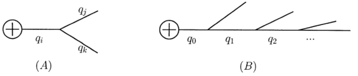
matrix element becomes large. In particular, this is associated with emissions of soft or collinear particles. To be more precise, let us consider a particle i with momentum qj coming from some hard scattering that happens at energy scale

Q,

branching into two particles

j

and k with momenta qj and qk, see Fig. 1-1-(A). Be-cause of the internal propagator, the amplitude (A) of this process is proportional to

1/q2 and in the limit where the mass of the particles

j

and k is zero, we have

1 1

A ~1j - = (1.2)

q2 2E3 Ek (1 - cos 0)

qj

qi qo q1 q2

qk

(A) (B)

Figure 1-1: (A): branching of particle i to particles jk; (B): strongly ordered limit where q

>

q2

>

q2 > ... , this implies that each emission is more collinear than the

previous one.

where Ej and Ek are the energies of the particles j and k, and 0 is the angle between q'j and q'. From Eq. (1.2) we see that the amplitude gets enhanced when Ej or Ek --+ 0, or 0 -+ 0. In the first case the particles emitted are called soft because of the low energy, while in the second case they are called collinear because the particles are close to each other. A key characteristic is that in the collinear limit the cross section factorizes

dox+k -- dz 2 Pi -+jkd'x+i, (1.3)

qi

where dox+i is the cross section to produce the particle i inside some larger process X, dux+jk is the cross section to produce the particles jk, and P is called "splitting function" and represents the probability of the particle i to split into particle jk and can be calculated perturbatively in as. As an example, for a quark splitting to a quark and a gluon (q -+ _{qg) after averaging and summing over spins, at leading order}

in as, this is

P(O) _q-+qg = ₂₇ C F ₁ 1.4)

- Z' ₁₄

where z _{is the momentum fraction of the emitted quark with respect to the parent}

quark and CF = 4/3. If we integrated Eq. (1.3) over q2, we would get a large logarithm

log(Q/q). We can extend this argument to the emission of an arbitrary number of

where

2 2 2(15

q > q > q (1.5)

Condition Eq. (1.5) is equivalent to qoL

>

qa

>>

q2 > ... where I refers to the perpendicular component of the momentum with respect to the momentum of the mother particle. This means that in the strongly ordered limit, each emission is more collinear than the previous one, as depicted in Fig. 1-1-(B).

We saw that P(O) gives the probability for a parton to split. Using the Altarelli-Parisi equation it is possible to prove that the "Sudakov Factor", A(q2, qO), gives the probability of a parton to evolve from qO to q2 without branching [44], where

A(q

2

_{, q}

_{) =}

_exp

-

2

_d

2

I

_d

_z

as

P

_(z)

_.

_(1.6)

L

2q

q

27r

We can use the splitting function and the Sudakov factor to construct an algorithm that branches a parton i into two partons

jk

and then iterates this process to produce an arbitrary number of partons in the final state. This process is called a parton shower and can be implemented in a Monte Carlo simulation as an event generator. Whereas a fixed order calculation is based on the perturbative expansion of a, the parton showers is defined in the soft-collinear limit and uses a probabilistic Markov chain of 1 -+ 2 particle splittings to recursively generate partons. In this way we resum the LL contributions by systematically treating real parton radiation.

To study an event in a hadron collider both fixed order calculations and parton shower event generators are used. We generate an event in three phases [401. First we select the hard process at the parton level with a probability proportional to its production cross section, calculated using standard fixed order perturbation theory. Second, the produced partons, which are taken to be highly off-shell at the hard scale

Q,

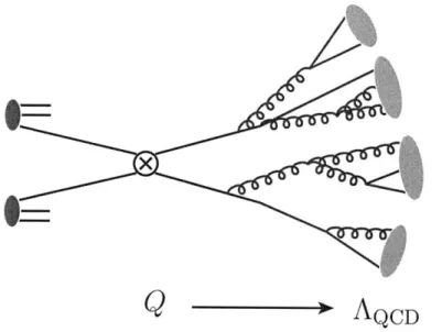
radiate additional partons using an event generator and evolve down until their off-shellness reaches the hadronization scale AQCD. Finally, all the partons hadronize using a confinement model. We illustrate these three phases in Fig. 1-2 for

Q

AQCD

~

Figure 1-2: ppi collision with final shower: two partons taken from the protons (red blobs) interact at scale

Q.

parton showers is used to emit radiations from

Q

down to the scale AQCD where the partons hadronize (blue blobs). There is also radiation from the initial partons and from the remnants of the protons (not shown).

a pp collision. Two partons taken from the protons (red blobs) interact at scale

Q

producing two partons. A parton shower event generator is used to emit radiation from

Q

_{down to the scale AQCD where the partons hadronize (blue blobs). There} is also radiation from the initial partons and from the remnants (not shown); these are also described using a parton showers approach. Monte Carlo event generators like Pythia [91, 92] or Herwig [5, 38] are heavily used by experimentalists to simulate these types of events and have proved indispensable for making exclusive theoretical predictions.

There have been several improvements to LL parton showers such as MC@NLO [52], or CKKW [31], but a systematic way to resum NLL is missing in the literature and there is not even a clear method to catalog all the necessary corrections. The main problem to include NLL corrections is that we have to take into account emissions that are not strongly ordered, where q

>

q i and where the factorization formula Eq. (1.3) is no longer valid. This means that we have to consider interference between different amplitudes as well as spin and color correlations.

using SCET to pave the way for an implementation of a NLL parton shower algorithm. SCET is an appropriate effective theory for studying parton showers because it is designed to reproduce exactly the limit of soft and collinear particles. Moreover, SCET is organized in an expansion of a power counting parameter that makes it possible to classify all corrections to a known order in this parameter. The first work on parton showers using SCET was Ref.

[17],

where the authors proved how the splitting function and the Sudakov factor emerge naturally in SCET. They reproduced the LL parton showers using SCET but they introduce choices and approximations at several points which makes prohibitive to calculate corrections.

In our work, we describe the parton shower using a tower of independent but related effective field theories that we call SCETi. Each SCET is a soft-collinear effective field theory. The difference between SCETi and SCETi+1 is that SCETi+1

describes collinear particles with virtuality that is much smaller than the virtuality of a collinear particle in SCETi, that is if qi+1 is a generic collinear particle in SCETi+1

and qi a generic collinear particle in SCETi we have that q,+1 < q. We describe

each emission in the strongly ordered region using a different SCETi. Even if we have many EFTs, we will use only a single power counting parameter that we call A. The LO operator in A for n partons describes n emissions in the strongly ordered region. To resum NLL we need to calculate the NLO operators in A as well as correction in a. In this work we will focus on corrections of the power counting, but in our framework we can also calculate corrections in a,. We find two different kinds of corrections at NLO in A: scattering corrections and jet-structure corrections. The hard-scattering corrections depend on the hard-hard-scattering process being investigated. The jet-structure corrections are independent from what happens at the scale

Q,

hence

they are universal in the sense that they are the same for each process we want to study. The SCETi picture, besides defining a clear method to calculate NLO corrections, has another important advantage in that we have factorization between emissions also at NLO. This characteristic is a crucial ingredient that gives hope for a future construction of a NLL parton shower algorithm.

of SCET, called reparametrization invariance (RPI). Part of this thesis is devoted to study RPI. Symmetries are fundamental tools in all fields of physics. Knowing that a quantity is invariant under a set of transformations allows us to make some predictions. For example, if we have a quantity that depends only on two vectors, pl and qP, and we know it is a Lorentz scalar, we can immediately say that it can be only a function of q2_{, p}2 _{and p - q. Similarly, knowing that SCET is invariant}

under RPI, we are allowed to express all quantities in SCET using a complete a set of RPI invariant objects. In this thesis we construct operators that are invariant under reparametrization. Using RPI operators will turn out to be very powerful method to find a minimal basis that is homogeneous in the power counting in particular for processes with multiple jets.

1.4

Outline

In chapter 2 we give a brief review of SCET. After describing the main ingredients of SCET, we define RPI in this context. In chapter 3 we construct a set of operators that are invariant under reparametrization. It is based on Ref. [80]. We can use this set to reduce the number of operators in SCET. We construct a minimum basis of pure glue operators for DIS at twist-4, for production of two and three jets from

e+e~, and for production of 2 jets from gluon fusion. Chapter 4 is dedicated to parton showers and is based on Ref. [21]. We formulate the shower emissions as a standard matching procedure between different SCETi, namely SCET -4 SCETi+₁. We use this formulation to classify and compute various corrections to the shower. Conclusions are given in chapter 5. We leave many of the technical details to the appendices.

Chapter 2

Soft Collinear Effective Field

Theory

2.1

Introduction to SCET

Soft Collinear Effective Theory (SCET) is an effective field theory of QCD that de-scribes the interactions of collinear and soft particles [8, 10, 14, 18]. The momentum p of any particle can be decomposed along two light-cone vectors, n and ii, with n 2

= 0,

2= 0 and n 2, as

pe =n-p-

+p-

+p_,

(2.1)

where p = i p and the particle's invariant mass is p2 _{= p+p + p2. We use a}

Minkowskian notation for p =

-2

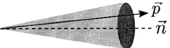
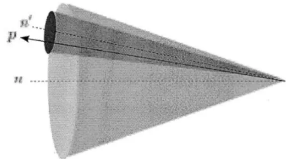
, where 'l is Euclidean. SCET's degrees of freedom include collinear and soft fields. 1

A particle is collinear to a direction n if its momentum scales as:

(n -p, , p±) - (A2, 1, A) p , (2.2)

'Our primary interest here is the perturbative structure of jets, so we use what in literature is often called SCETJ theories with collinear and ultrasoft modes. For simplicitly we will always use the phrase soft in place of ultrasoft.

Figure 2-1: In SCET, a particle with momentum p is collinear to the direction n if P is inside a cone centered in n' and of angle A.

where p ~

Q

is the hard scale, and A < 1 is the power counting parameter of the SCET. Pictorially, we can think of a particle collinear to the direction n as having its three-momentum jis inside a cone centered on n' and of angle A, see Fig. (2-1). A particle is soft if

(n - p, P, pi) ~ (A2_{, A}2_{, A}2₎ Q. (2.3)

Both Eqs. (2.2) and (2.3) imply p2 QA2 2.

We obtain SCET from QCD by expanding in powers of A, integrating out the hard modes and dividing the quark and gluon fields into separate soft and collinear modes. The soft fields are ( (x) and A,(x) where OP ,(x) ~ OP A,(x) ~ A2. For the collinear case, we introduce a momentum-space lattice and we give each field an index-label describing which lattice vector it is collinear to. To divide the QCD fields in this way, we split the momentum of a collinear particle into a "large" part

#3I

and a residual

one k' ~ A2

pA = Y+k" , where P" = n-p- ₂

+

p- I. (2.4)

We can remove the large momenta

P

from the fermion field by the Fourier transform

V(X) = e~-x Vn,p (2.5)

For a collinear particle along n, Ot'8n,P(X) - A2. The four component field, on,,, has two large components (n, , and two small components , that are defined using the

following Dirac-space projectors:

L

np+ L# ~ ±b + (2.6)

These satisfy the relations

4 = (jap ) = 0 . (2.7)

4

We can also similarly define a collinear gluon field A",(x) whose fluctuations are characterized by the scale of its residual momenta, q2 _A2_{. Pictorially, we can}

think of (n,p and A", (x) as fields that create a particle whose three-momentum lies inside a cone with opening angle ~ A about the three-direction n'. We define Pn as the momentum operator that picks up the large component of the momentum: ?n(n,p(x) = 3'# n,(x). Collinear fields always appear with a sum over P, so it is useful to redefine the fields as

n= ei(x~ , A -= ei44xA,. (2.8)

The leading order SCET Lagrangian is

£C(O) 'C()' (0)(29

SCET -5 n.. 29

nE{n }

where E42) has only collinear interactions among particles collinear to the same n. Particles collinear to different directions can interact either by the exchange of soft modes in 4), or from their coupling to other sectors in external operators. Two collinear sectors in SCET, ni and n2, are distinct if [9]

nin2> A2 , (2.10)

Thus the key defining concepts of an SCET-theory are its hard-scale

Q,

its collinear sectors

{[n]},

and its power counting parameter A which governs the im-portance of operators and size of the collinear sectors.

We define collinear covariant derivatives as

in-Da= 4+gn-.,,, DL" = Pn4+gA-L,, in-D =in-8+gn-An,,(.1

where Pn is the momentum operator that picks up the large component of the mo-mentum, that is Pnp,n = Pp ,,. When integrating out hard offshell fluctuations and constructing gauge invariant structures in SCET, it is necessary to include collinear Wilson lines, Wn, defined by [14]

Wn (X) = [E exp (_ i- An,,(X) .(2.12)

perms

The collinear fields AP, are defined with the zero-bin procedure [78]. To couple soft degrees of freedom we define an soft covariant derivative

iDf = i&0+ gA , (2.13)

that can act on collinear fields. At lowest order the coupling to n-collinear fields in-volves n-De and can be removed from the Lagrangian by the BPS field redefinition [14]

2,,(X) - Yn(x)(n,,(x), An,q(x) -+ Yn(x)An,q(x)Y'(x), (2.14)

with the soft Wilson line

0

Yn(x") = P exp (i g ds n -A, (x" + sn")). (2.15)

This field redefinition allows us to organize power corrections as gauge invariant prod-ucts of collinear and soft fields as we discuss in the next subsection.

inte-grating out the field, s. At LO, we have [10, 18]

L(4) =

(in-+gn-A

+ i I Wi

)

, (2.16)

where we intrinsically sum over the large, label momenta,

P,

as well as the collinear index, n, which we have kept explicit as a label. The LO collinear Lagrangian for gluons is given in [14].

Operators are formed from products of the above fields, and the power counting for an operator is determined by adding up contributions from its constituents. The power counting for the fields and derivatives in SCET is

(n~ A, i m ~A2, 3_, Ws~Y ~A . As ~ A2 ) (2.17)

2.1.1

Gauge Invariant Field Products

To build operators in SCET we want to use structures which are gauge invariant and homogeneous in the power counting. For SCET a convenient set of gauge invariant structures are:

Xn =Wt' , DP - WnD/-W ,, (2.18)

together with the ?P label momentum operator and derivative operator jIBL acting

on these structures. The collinear fields in Eq. (2.18) are the ones obtained after the field redefinition in Eq. (2.14). It is convenient to be able to switch the collinear derivatives multiplied by Wilson lines for gauge invariant field strengths, for which we use

inD = Pn-+

gBn-B

,

iri*Dn = iri.O+gn-13n, in-.5n = i.0- gn*Bn,(.9

(n -An, ih-An, AZ)~ (A2 11)

(M -0 A-p 7Pnj 2,(A1,1A), I

ki

jPq 1 f

no

6n

6

ROn

(1)

(11)

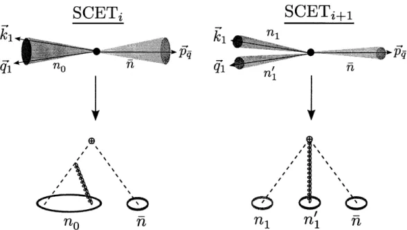
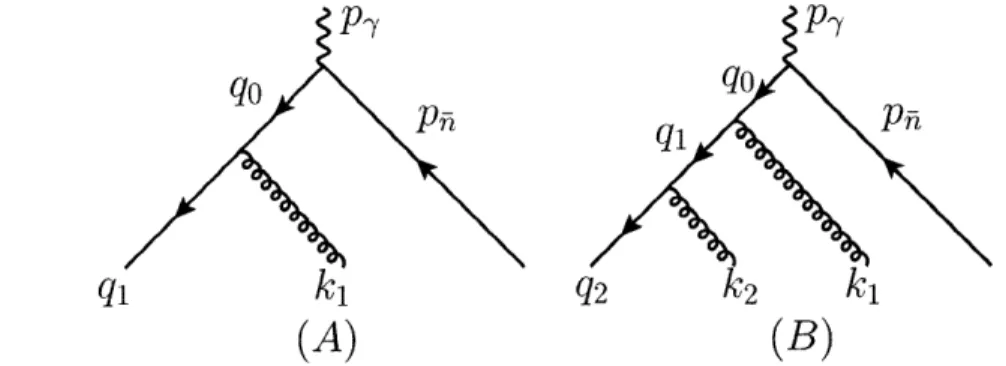
Figure 2-2: Final state with a quark (q1), antiquark (pg), and gluon (ki). Different kinematic configurations are described by different SCET operators. In (I), the quark and the gluon are collinear to the direction no, represented by their sharing a cone. In (II), the vectors qi and ki are too far apart to be collinear. The Feynman diagrams below show that collinear fields can come from the Lagrangian vertices, but non-collinear ones arise from higher-multiplicity operators.

and note that

ni-D

= P,. Here the field strength tensors are

-E-~ 1 -- 1220

gB 1 = [I-[inz-D, iDn4] , gn-3 [=-[in-Dsin-D]], (2.20)

where the label operators and derivatives act only on fields inside the outer square brackets, and g!3? and gn-B are Hermitian.

We can construct gauge invariant operators using the fields defined above. Since the collinear fields carry a label referring to a specific light-cone vector, these operators describe particles in a specific region of phase space. SCET therefore distinguishes situations with the same number particle but different kinematics using different op-erators. For example, one can take an amplitude for three external particles: a quark (q1), a gluon (ki) and an antiquark (pq). We can consider two different configurations that we call |qngnog) and |qngn'qig). In the first, shown in Fig. 2-2(I), the quark

and the gluon are no-collinear, and the antiquark is collinear to a different direction, i. Here the amplitude is described by operators with two distinct directions, say

vnoFXn ~ A2_{, n.g}3 _{' IF'Xn ~ A}3

_,

_(2.21)

(where the form of the Dirac structures F and ' are not central to our discussion here). The first operator in (2.21) can emit ii - Ano gluons from the Wilson line in Xno _{but requires a Lagrangian insertion to emit an AJ- gluon. Schematically the} amplitude for a transverse gluon has contributions

A'

=

d

{0|T

L (0)(x)

nX 1'Xa(0)|quqgne +

(0)

X

no

(2.22)

In Fig. 2-2(11) each of the particles is collinear in a distinct direction, so no cone of size - A fits two of the momenta. In this case, the amplitude can only come from an operator with three distinct directions, such as inB ,'Xn:

A" = (0OlnigB P"Xalq.g gn) (2.23)

2.2

Reparametrization invariance

When a set of fields have their largest momentum component in a light-like or time-like direction then the structure of operators built from these fields is constrained by reparametrization invariance. This invariance appears due to the ambiguity in the decomposition of momenta in terms of basis vectors and in terms of large and small components, in other words reparametrization constraints arise because the decomposition in Eq. (2.1) is not unique. We can shift n by a small amount and still have a suitable basis vector for the particle. We also have a large amount of freedom in the choice of i. For each {n, } pair the most general set of RPI transformations

which preserves the relations n2 = 0, i 2 = 0, and n-i- 2 are

M ,

- n,

+

A

n,

n,

n,

(1+a)

+-

n,

ii - n,

fi

Ihn, + E s

1

->(1 -a) 6,

where the five infinitesimal parameters are

{A-,

e1, a}, and satisfy ii-e = n -e =

h -A' = n -AL - 0. The transformations (I), (II) and (III) in Eqs. (2.24) are called RPI-I, RPI-II and RPI-III. To ensure that n provides an equivalent physical description of the collinear direction for these particles requires the power counting {A L, e7, a} {A1, A0, AO} [77]. Thus n can only be shifted by a small amount, while parametrically large values of a and El are allowed. This is because the vector n has physical meaning,

i+

is the direction where most of the momentum is allocated, that is the direction

7t

is inside a cone centered on

-R4

with on opening angle ~ A. The RPI-I transformations moves n inside this collinear cone. T does not carry any real physical meaning and it is only needed to decompose the momentum in (2.1). The collinear sectors {n} in SCET are really equivalence classes of null vectors,

{[ni]},

where an equivalence class [n] is defined as

[nj] = {n E [nj]| n - nj ;< A 2}1 (2.25)

The class [nj] consists of all light-like vectors connected to n' by a type-I RPI trans-formation n- ±4nA + A"1

The type-III boost simply ensures that (#Nni) - (#Nni) - (#Dni) + (#DFi) = 0 for each i, where (#Nni) counts the number of ni factors in the numerator of an operator, (#Dni) counts the numbers of hi factors in the denominator, etc. With three collinear directions an example of a type-III RPI invariant parameter is

ni -ni2 ln3

(2.26)

n2 naF1

The type-I and type-II transformations of collinear objects are more interesting and are summarized in Table 2.1, which we take from Ref. [77]. Since the factors induced

Type (I) Type (II)

n2 -+ A n -4 ni

i~i hii + ii+

n-Da -+ n-D + AL-Dy n-Da -+ n-D

n-+ n -2 D A -D I D" -+ 1" -- n-D - -D

n-Dn -+ n-Dn n-Dn A-Dn +E1 -D

W -+W

W

-+

[(i-.1

_ e -D)Wj

Table 2.1: Summary of infinitesimal type I and II transformations from Ref. [77]. With multiple collinear directions these transformations exist for each {ni,

ni }

pair.

by these transformations occur at different orders in A, demanding overall invariance of a physical process provides connections between the Wilson coefficients of operators at different orders in the expansion.

When we couple collinear and soft particles there is another ambiguity, associated with the decomposition of a collinear momentum into large and small pieces. If the total momentum P of a collinear particle is decomposed into the sum of a large collinear pl and a small soft momentum k":

PA =p _{+ kA=-n( + k) + 2n-k + (pi + k_),}

2 2 (2.27)

then operators must be invariant under a transformation that takes r-p -+

n-p

+

-,

p -+ p" + l, i - k - k - h - f, and kl -± k" - f". To construct invariant objects that have nice gauge transformation properties we use the combined covariant derivatives [15, 25],

iD'n-

+ WniD/' Wt, in-Dn + Wiii-DsW. (2.28)

This can be implemented by taking

and then expanding in A. The results in Eq. (2.29) give powerful relations as they re-late the coefficients of operators involving collinear fields to those involving soft fields. These relations are quite easy to derive order by order in A. Note that reparametriza-tion constraints associated with transformareparametriza-tion of the soft Wilson line Y are auto-matically enforced by the other constraints.2

2

For example, prior to the field redefinition only the combination in-D = in-O + gn-A, + gn-A,

appears acting on collinear fields. A type-I transformation connects this to a D#, and Eq. (2.29) then connects this to the same iD± that one would find by direct transformation of Yn.

Chapter 3

Reparametrization Invariant

Collinear Operators

3.1

Introduction

To study a process using SCET, the standard procedure is to take the QCD current,

JQCD, underlying that event and to expand it in terms of SCET operators using an

operator expansion:

JQCD

CO,

(3.1)

where C₂ are the Wilson coefficients describing the physics at the hard scale, and O

are the SCET operators that reproduce the infra-red (IR) behavior.1 _{The process}

of calculating the Wilson coefficients is called matching. All the operators in SCET have a power counting in A, and the OPE is organized as an expansion in A. In order to fully reproduce JQCD, we have to match it to an infinite tower of SCET

operators with higher and higher power counting, but at a given power of A, the number of operators is finite, and we only match JQCD _{to SCET operators up to a}

fixed order in A. To construct the expansion (3.1), the standard procedure is to build

1 _{We will see in the next paragraph that the product of Wilson coefficients and operators in}

a gauge invariant basis of operators with a definite power counting, using the gauge invariant fields defined in Section (2.1.1). We call leading order (LO) operators, QOi, the operators in (3.1) with the lowest power counting, next-to-leading-order (NLO) operators, ONLO, the operators with the next higher power counting and so forth. Thus we can write (3.1) as

JQD= ECL00LO + CNLOoNLO

JQCD + +..(3.2)

SCET is invariant under reparametrization invariance, thus we have

6RPI (Cii) = 0, (3.3)

where with 6

RPI we indicate the set of transformations in table (2.1). We can solve

the Eqs. (3.3) order by order in A and find relations among Wilson coefficients, and because the transformations in (2.1) occur at different order, Eqs. (3.3) allow us to relate Wilson coefficients at different order. In other words, we use RPI transforma-tions to reduce the basis of operators that we need for the matching. Because the reparametrization invariant transformations depend on the collinear direction n, if we have operators with different directions, we have a different set of transformations for each n. Thus when dealing with operators with multiple directions,

solving

Eqs. (3.3) becomes hard, if not prohibitive.

In this chapter we will construct RPI operators Q*, which are reparametriza-tion invariant, that is 6

RPI(Qi) Q The results of the chapter were presented in

Ref. [80]. The operators Q' are made of reparametrization invariant fermion fields

X', and gluon fields gP", that we call superfields. The superfields are made gauge

invariant using a reparametrization invariant Wilson line W that is the generaliza-tion of the usual Wn. These objects do not have a definite power counting order, in particular we will know the order in the A-expansion where they start, but they will contain terms at all higher orders as well. We build a basis with these RPI and gauge invariant objects, which is made minimal using equations of motion and

kinematic constraints as discussed below in Section 3.4. Each element of this basis is assigned a Wilson coefficient, and then the elements are expanded to find the final basis with elements of a definite power counting. In this way we immediately obtain relations between Wilson coefficients of operators at different orders. Once we expand and check for redundancy, the number of independent Wilson coefficients is equal to the number of independent RPI operators in the reduced basis. We will apply RPI operators to construct the minimal basis of operator for several processes.

In hard-scattering processes, DIS provides a familiar context where the construc-tion of a minimal operator basis requires judicial use of the quark and gluon equa-tions of motion, and an invariance under reparametrizaequa-tions of a light-like direc-tion [41, 42, 62, 63, 86], for a review see [64]. The invariance under reparametriza-tions becomes more valuable at higher orders in the expansion, being particularly constraining on the basis of twist-4 operators derived in Refs. [41, 42, 62, 63]. We derive RPI constraints for collinear operators in DIS and compare to these classic results as a test of our setup. For DIS the minimization of the basis of RPI operators is quite similar to the reduction of operators in Ref. [63]. On the other hand the basis of SCET operators are comprised entirely of analogs of "good" quark and gluon fields, namely a two-component quark field Xn and just two components of the gluon field strength, B. These objects both incorporate Wilson lines, and for these operators it is easier to find a minimal basis. The RPI relations provide Lorentz invariance connections between the Wilson coefficients in this basis. These constraints carry a process independence, they depend on the type of operators being considered, but not on the precise process in which they will be used. It should be emphasized that when matrix elements are considered for a particular process, a further reduction in the number of independent hadronic functions becomes possible. For twist-4 quark operators in DIS this type of further reduction was discussed in detail in Ref. [42] and for inclusive B-decays in. [95], but this type of reduction is not our focus here.

Our construction is general enough that it applies not just to DIS like processes, but to operators with multiple collinear directions, which are useful for processes with multiple hadrons and jets. These operator bases provide a starting point for deriving

appropriate factorization theorems for different processes. The invariant operator procedure becomes more and more efficient as the number of directions grows.

The outline of this chapter is as follows. In subsection 3.2 we study the convolu-tion between Wilson coefficient and operator. We divide hard interacconvolu-tions into two categories, those with an external hard leptonic reference vector q", and those where the hard interaction is between strongly interacting particles. Since most SCET ap-plications focus on the former case, we address some of the additional notational complications that occur for the latter. A set of RPI invariant collinear objects is constructed in subsection 3.3, followed by a summary of identities that can be used to reduce the operator basis in subsection 3.4. The inclusion of mass effects is considered in subsection 3.5, and the expansion of the RPI objects is carried out in subsection 3.6. Applications for constructing operators are considered in subsection 3.7. In subsec-tion 3.7.1 we verify that our approach provides a simple way to reproduce the known RPI result for the chiral-even scalar current given in Ref. [581. In subsection 3.7.2 we construct a general basis of field structures involving up to four active quark or gluon operators, and with up to four distinct collinear directions. In subsection 3.7.3 we consider the special case of quark operators for DIS at twist-4 with one collinear direction, and compare with the literature. In subsection 3.7.4 we derive a basis of op-erators for pure gluon scattering in DIS up to twist-4. Finally we apply the formalism to jet production. In subsection 3.7.5 we demonstrate that very little information is gained about the operator basis describing e+e- - 2 jets. In subsection 3.7.6 we show that RPI turns out to be quite powerful for constraining the e+e- -+ 3jet operators. Finally we show that RPI is also useful for two jet production from gluon-fusion,

gg -+ qq, and we construct a basis of operators for this process in subsection 3.7.7. Conclusions are given in subsection 3.8.

3.2

Convolutions

In the presence of collinear fields, a hard interaction can introduce convolutions in variables wi between the perturbatively calculable Wilson coefficient C(Q2, wi) and the

matrix element of the collinear operators. In this case the amplitude, cross-section, or decay rate has the form

A = J[dwi- -.- dW] C(Q2_{, w) (O(wO)).}

(3.4)

The convolutions occur because a component of the hard momentum and of one or more collinear momenta are O(A0). The exchange of momentum between the hard and collinear components yields a convolution in variables wi, where the number of such variables is constrained by gauge invariance and by momentum conservation in the matrix element. A gauge invariant momentum from the collinear fields can be picked out by a delta function acting on one of the collinear objects in Eq. (2.18), such as [6(w - -P)X, and traditionally in SCET a subscript notation is used for these products,

-n

~ -tnXn ~ip,,,=[

(g[3' [gB

o(o

-

P

),

(gn- B)W [gn-Bn

6(W

-

).

(3.5)

We will refer to these as homogeneous objects since they have a definite order in A, and call the operators build from these objects homogeneous operators. As an example we have the bilinear scalar operator,

O(wi, w2) = xn, Xn,W2 (3.6)

When we consider RPI it will be convenient to use different 6 functions and con-volution variables c', that are type-III invariant. Essentially each T =

n-Pn

must be multiplied by a scalar transforming as n under RPI type-III. There are two cases to consider:

i) situations where there is a reference vector q" for the hard interaction, |q2

Q

2

_>

_{AQCD, which is external to the QCD dynamics,}

par-ticles.

Case i) applies to examples such as DIS where q" is the momentum transfer from the virtual photon, or e+e- -+ jets where q' is the four momentum of the e+e- pair. Here we can use n.q - A' to make the 6-function type-III invariant for n-collinear fields. Since Q2

>

AAQCD > AQCD we know that n - q

>

n -p, where p is the momentum of a collinear particle in the jet. Thus we use a variable LZ with mass dimension two, and will find 6-functions of the form2

6( - n -qPn) . (3.7)

We also introduce a subscript notation with hatted variables,

(gB21)L g 6 Pg

(-

n -q

)

, (gn -Bn)c , gn-B, o(0-n-q

)

(3.8)

Since 5(w^ - n - qPn) ~ A0, it is leading order in the power counting. Furthermore,

we have 6(Ci - n - q P) = 6(c/n - q - P)/n - q, so identifying C = n -q W there is no real change to the structure of Eq. (3.4). An operator built out of the components given in Eq. (3.8) has multiple labels, 0 1,2, . . .), and the Wilson coefficient for the

operator will be a function of the same parameters, C(0 1, C2, ... ), yielding Eq. (3.4) with C's replacing o's.

For processes in case ii) there is no analog of the external q". Examples here include pp -+ jets, or any other hard process that does not involve external leptons or photons. The key difference with case i) is that here the hard interaction must involve two or more collinear directions, so we are guaranteed that there are scalar products ni -ni ~ A0. For this type of reaction the type-III invariant 6-functions which are

convoluted with Wilson coefficients always involve large momenta for two different

2 For B-decays these type-III invariant 6-functions were used in Ref. [85], with q" ~ mbv",

J(O - n-q P,) = 6(C - mbn-v P,) = 1/mb 6(6' - n-v T), where c = mbw'. This form of invariant 3-function was also quite useful for analyzing the factorization theorem for e+e- -+ J/4VX in Ref. [49].

collinear directions,

1 -

-Ai =

J

Q

ij

- ni -nj'P,) . (3.9)

Here Pn acts on a gauge invariant block of ni-collinear fields, and Ps, acts on a block of nj-collinear fields. Since this 6-operator does not act on a single block of collinear fields we will not use a subscript notation like Eq. (3.8) for Coig. In this case the structure of the factorization theorem between operators and Wilson coefficients is a bit different than in Eq. (3.4). For example, consider an operator with collinear objects for four directions, where the convolution is

[J

dij] C(C)i)j[fJ

Akm] x a(gB37

) (gBf,)xna.

(3.10)

ij km

Here the products are over the six unique pairs ij with i

$

j,

and Pn, in the Akm acts on the ni-collinear field(s). The convolutions in Eq. (3.10) can be manipulated into the form of Eq. (3.4) by inserting four factors of 1

f

dwi J(wi - Pn), writing g = J(cjij - n -m n wiwj/2) and carrying out the integrals over the six CQij's to give

[dwi

-..

dw4]

C(ni -n wioj)

4nw,(gB

w)(gB,-,,4)xn2,2.

(3.11)

Here the RPI-III transformation of the measure cancels against that of the 6-functions in the operator, and RPI has constrained the Wilson coefficients to only depend on invariant products

ni -n2WiW

2, ni-n3xios, etc.

Due to the simplicity of the soft-collinear coupling at leading order in SCET a further factorization of the EFT matrix element can be made into collinear pieces J, and soft pieces S at each order in the power counting:

(O(oP)) =

J

dkj J(wi, kj) S(k). (3.12) However it is the factorization in Eq. (3.4) that will be central to our discussion of reparametrization invariant operators.

3.3

Construction of RPI and Gauge Invariant

ob-jects

We now construct reparametrization invariant objects in SCET whose leading terms give the fields in Eq. (2.17). These are then generalized to objects that are simultane-ously RPI and gauge invariant whose leading terms give the objects in Eqs. (2.18,3.8). For simplicity only collinear objects are considered in this section. Pulling out the large phases from the collinear quark field and gluon field strength, and decomposing the full theory field into independent collinear sectors we have at tree level,

7P(x) = ezX' ) ,(x)), G"(x) =3 e"xpG"(x) . (3.13)

n n

Full Lorentz invariance act on the fields @b(x) and GW' (x), but the RPI transformations that we are interested acts independently on each collinear sector labeled by n. Two sectors i,

j

are independent if ni -n

>

A2, and the sums in Eq. (3.13) are really over equivalence classes,

{n},

where a class consists of vectors related by RPI. From the discussion in section 2.2 the n-reparametrization invariant collinear quark and field strength are easy to identify

S+igG iD,iD"] . (3.14)

Under the transformations in Table 2.1 for

{n,

h}, the quark field

@n

remains invari-ant

[77],

while the gluon tensor is invariant because the vector DO is invariant. To make the fields in Eq. (3.14) invariant under the additional reparametrization trans-formations that link collinear and soft derivatives we replace in Dn a in -D+gn -A₈,

iD -+ iD4 + WaiDIW, and i - D -+ n Dn + Wnin - DsW. After this

re-placement the decoupling field redefinitions in Eq. (2.14) can be made. In Eq. (3.14)

gn = 0, and the term in On with a 1-covariant derivative corresponds to the two

components of the full fermion field that are small when p1 /A -p < 1. Since

##s

#

0,

A~ whereas ~ -.AnSh4

We also need reparametrization invariant 6-functions whose expansions reproduce Eqs. (3.7) and (3.9) at lowest order. For example, these are needed to construct an RPI operator which when expanded gives Xn,w4XnW₂ at lowest order. For situations

where there is an external hard vector q" the invariant 6-function is

Ai _= ( - 2q - i&n) = 6(6Z - ni -q P,,) +... , (3.15)

where as described in section 2.1.1, q" is a parameter specific to the kinematics of the process being studied. Notice that 6(c2 - 2q -i&n) starts at O(A0), is RPI, and is gauge invariant when acting on singlet operators. Here

n/- j

an/ - -Pn + P,_L + -in -an (3.16)

and functions of iBn ~ (A2 , 1, A) can be expanded in powers of A. Note that Pn and P'- are only non-zero when they act on n-collinear fields. It is useful to extend this property to the full iOn, which we can do by distributing an i&l derivative across all fields that it acts on, writing for example ia"@/-n1On2 = ('any, n)V'n1 2 + Onb (iO2 )n2). In some hard processes there is more than one external hard vector, and a natural question arises as to whether qP provides a unique choice for this construction. For example, in DVCS, -y*p - (*)p we have the momentum q' of the incoming y* and the momentum q'" of the outgoing 7(*). In appendix A we show that as long as

q - qL ~ A or smaller, the choice q suffices, since for the purpose of constructing

a basis of operators it is equivalent to the choice of any linear combination of q and q'. On the other hand, for situations where there is no external hard vector q", the appropriate RPI 6-function is

aij

= 6(i. - 2ia, - iBn) =(

-

!i .2 P , +±... . (3.17)

This 6-function operator acts on two independent collinear directions. In general we must include in an operator a set of Ai and Aij which are linearly independent. Once