Friction-induced self-organization of a one-dimensional array of particles

HAL Id: hal-01425278

https://hal.archives-ouvertes.fr/hal-01425278

Submitted on 3 Jan 2017

HAL is a multi-disciplinary open access archive for the deposit and dissemination of sci-entific research documents, whether they are pub-lished or not. The documents may come from teaching and research institutions in France or abroad, or from public or private research centers.

L’archive ouverte pluridisciplinaire HAL, est destinée au dépôt et à la diffusion de documents scientifiques de niveau recherche, publiés ou non, émanant des établissements d’enseignement et de recherche français ou étrangers, des laboratoires publics ou privés.

Friction-induced self-organization of a one-dimensional

array of particles

Farhang Radjai, Stéphane Roux

To cite this version:

Farhang Radjai, Stéphane Roux. Friction-induced self-organization of a one-dimensional array of par-ticles. Physical Review E , American Physical Society (APS), 1995, 51, pp.6177 - 6187. �10.1103/Phys-RevE.51.6177�. �hal-01425278�

Friction-induced

self-organization of a

one-dimensional array of particles

Farhang Radjai

H ochstleistungsrechenzentrum, Forschungszentrum, 524 25 Jülich, German y Stéphane Roux

Laboratoire de Physique et Mécanique des Milieux Héterogènes,

Ecole Supérieure de Physique et Chimie Industrielles de Paris, 10 rue Vauquelin, F-75291 Paris Cedex 05, France

We study the frictional motion of a linear array of parallel identical cylinders on a plane where all interparticle and particle-plane contacts can be described by a Coulomb friction law. The entire system can be characterized in its steady state by an effective coefficient of friction and an effective inertia, both varying with the external driving force. In the steady-state regime, the organization of the array appears as regions involving different rotation modes (sliding with no rotation, rolling on the support, alternate rotations, etc.). The mechanisms leading to this self-organization in modes are studied analytically.

I. INTRODUCTION

In the context of standard continuum mechanics, the only field needed to describe the elastic deformation of a solid body is the displacement field alone. Rotations do not appear. They can be computed indirectly from the rotational of the displacement field. Other elasticity theories have been developed in order to account for the rotational degrees of freedom of a solid material, such as "Cosserat" or "micropolar" theory [1]. Dimensional analysis shows that an intrinsic length scale À has to be introduced. This length may be interpreted as the scale below which rotations can significantly differ from those deduced from the rotation of the displacement field. At a larger scale, the difference vanishes, and thus upon coarse graining the standard theory is recovered.

In the case of granular materials, the discontinuous ge-ometry of the solid phase, and thus of the displacement field, makes it difficult to establish a direct connection between a discrete description at the particle level and a continuum homogenization at a large scale. In particular, the effect of individual rotations appears to play a deter-mining role [2]. Although the framework of Cosserat the-ory seems more suited to such media, it does not appear to provide a simple key to the analysis. Sorne attempts in this direction have been proposed [3]; however, basic questions remain, such as the identification of this intrin-sic length scale, which is often postulated to be a typical particle size. Other effects may motivate the study of rotations in granular media, such as the propagation of sound (5,6].

• Also at Laboratoire de Physique et Mécanique des Milieux Héterogènes, ESPCI, 10 rue Vauquelin, F-75231 Paris Cedex 05, France.

Considering only the rotations of particles, one major difficulty appears immediately: the generally disordered geometry of the packing of particles induces a "frustra-tion" of rotations. To mention only the two-dimensional case, as soon as a "loop" of contacting particles contains an odd number of elements, rotations of the particles in the loop are not possible without friction being mobilized on at least one contact. We employ the word frustra-tion in analogy to the physics of spin glasses, where the presence of antiferromagnetic coupling between neigh-bors makes it impossible to satisfy ali couplings simul-taneously. We will not try here to develop the compari-son between these two fields any further, although sorne suggestions along these lines have been proposed [4].

In this paper we consider a very simple system consist-ing of an array of disks in mutual contact supported by a plane. Two neighboring particles are in contact with the plane and thus a pair of particles and the support form a loop of three solids such that rotations are frustrated. Since frustration involves sliding on at least one contact, it is important to incorporate the friction law accurately in the description of the system. We will consider here the most basic law of friction, namely, Coulomb's law of friction.

When the array is pushed in the direction of its mean orientation, particles will move and rotate and a collec-tive organization of rotations will emerge. This organiza-tion is rather complex. In particular, it involves typical length scales w hi ch may be mu ch larger thau the parti cie size, depending on the coefficients of friction (interparti-cle and parti(interparti-cle-plane) and the confining pressure. This observation might motivate revisiting discrete-continuum transition through the analysis of intrinsic length scales different from the particle size.

In order to present our approach, we will first describe in Sec. II the simple case of a single particle being pushed on a plane. In Sec. III, we will consider the more gen-eral case of a long array and report on sorne numerical

simulations. In Sec. IV, we will study analytically the collective organization of the array and describe the dif-ferent phases observed. We will discuss the transition between the different phases and the expected effects on the global motion of the entire system.

II. THE CASE OF A SINGLE PARTICLE Consider first the geometry illustrated in Fig. 1: A single disk supported by a basal plane is pushed by a constant horizontal force N. The mass and radius of the particle are assumed to be unity. The acceleration of gravity is set to unity as well. All quantities are normal-ized with respect to these natural units of the problem and, in particular, the moment of inertia I is a mere ge-ometrie constant. The friction between the particle and the support is assumed to obey Coulomb's law with a friction coefficient J.L1

• The friction between the particle and the pushing block also follows Coulomb's friction law with a coefficient J.L· The translational and angular veloc-ities of the particle are called v and w, respectively. We are interested in the steady-state regime, where the ac-celeration is constant. All solids are assumed to be rigid, and thus they cannot interpenetrate. Figure 1 gives the convention used for the orientation of the forces. The tangent force at the parti de- block contact is called T, whereas the friction force on the support is S. The nor-mal reaction of the support is R.

The equations of the dynamics are the following:

v

= N- S,

0 =

R

- 1-

T

,

lw = S - T,

(1)

where the fust two equations refer to Newton's law of motion in the horizontal and vertical directions, and the last one accounts for the rotation.

To find a complete solution to the equations of dy-namics, we need two more equations prescribed by the friction law at the two contact points. A friction law is a

T

J.1.N

v

- J.1.N1

-FIG. 1. Geometry of the single-sphere problem.

relation between the friction force and the relative tan-gential velocity at the contact point between two solids. The graph of this relation for Coulomb's law is displayed in Fig. 2. In two dimensions, it is written

Vr = 0 ::} T E [-J.LN 1 J.LN] 1

Vr

>

0::} T = -J,LN,

Vr

<

0 ::} T = J.LN 1

(2)

where Vr is the relative tangential velocity and T and N are the tangential and normal components of the contact force. ln the case where Vr = 0, there is no equation relating the tangential force to the normal contact force. In the present case of a single particle, we will consider different configurations with different relative velocities at the contact points and we will show that the friction force is always uniquely determined. In the next section, we will discuss a more general formulation of Coulomb's law adapted to dynamical systems [7].

There are two particular values of rotation velocities:

w 1

=

0 and w2 = v. Depending on the relative position

of w with respect to these particular values, the tangent force at the contacts will assume different values. How-ever, up to a change in the origin of time, the position of

w with respect to the key values Wi can be equivalently analyzed through the relative positions of the accelera-tions

w

with respect to Wi, since we are interested in the steady state, where the accelerations remain constant in time. Five different cases can be distinguished.

(1)

w

>

v.

In this case, we have T = J.LN and S =

- J.L' R. Since both tangent forces, T and S, contribute to a torque opposite to w, the angular acceleration has to turn negative. Therefore, no steady-state solution can be found.

(2)

w

=v.

In this case, T

=

J.LN, but S cannot be de-duced directly from Coulomb's law. However, the kine-matic constraint

w

=

v

suffices to determine the system entirely. The complete solution is written

T = J.LN, R

=

1

+

J.LN,

s

=

U

t'î

)N

,

(3)

. -

(1-~-') N W - l+I .

For this solution to be acceptable, the condition

ISI

<

J.L1

R has to be satisfied. This gives a constraint on the value of N:

J.L'(1

+

I) N

<

N 1 = - - - '

'----'---,-=---,-I

+

J.L- J.LJ.L'(1

+

I) (4) (3) 0

<

w

<

v.

ln this case, T = J.LN and S = J.L1

Ras given by Eq. (2). The complete solution of the system is

s

T

=

J.LN,

R

= 1 + J.LN, S = J.L' (1

+

J.LN), v = - J.L'

+ (

1- J.L1 J.L)N,

w

=

t

(J.L' - (1 - J.L1 )J.LN) .

(5)

Compatibility of this solution with the conditions 0

<

w

<

v

sets the following constraints on the values of N:

(6)

(4)

w

=O. ln this case, S

=

J.L1 _R

while T is not deter-mined by the friction law directly. The condition

w

= 0, however, gives an additional constraint which leads to

T

₌

_L_ 1 1-J-1.''

_v

= N-_E_ R

₌

_1-f'' 1 1- 1-'''

w

=

o.

s

= _ E _ 1-1-''' (7)

The condition JTJ

<

J.LN implies

(8)

(5)

w

<

O. In this case, S = J.L1

R and T = -J.LN. As

in the first case, the two tangent forces contribute to a torque opposite to w and thus no steady-state solution is

possible.

ln this way, the dynamics of the block-particle

sys-tem show three possible steady-state phases: rolling (phase 1), rotating and sliding on the plane (phase 2),

and sliding on the plane without rotating (phase 3).

Fig-ure 3 shows the friction forceS at the particle-plane con-tact as a function of the driving force N. The former increases linearly with the applied force in the two fust phases to saturate to a value greater than J.L1

in the last

one.

As long as the translational motion of the particle is of interest, these results can be compared to the dynamics

of a rigid block of mass m, pushed by a force N. The

respective equation of motion is written

0.30 0.25 0.20 Cil 0.15 0.10 0.05 0.00 0.0 1.0 2.0 3.0 4.0 N

FIG. 3. Evolution of the particle-plane friction force as a

function of the driving force N. Ali forces are normalized

with respect to the weight of one particle (see text). The first regime N

<

N1 corresponds to rolling on the support,

the intermediate regime N1 < N < N2 corresponds to partial

rotation where both contacts are sliding contacts, and finally

in the last regime N

>

N2, the particle slides on the support

with no rotation. Here, J.L = 0.1 and J.L1

=

0.2.

N-Mm = mv,

(9)

where M is the coefficient of friction at the black-plane

contact. Now, a look at the steady-state solutions of the single-particle problem [Eqs. {3), (5), and (7)) in different regimes shows that they can ail be written in the canon-ica} form of Eq. (9) if we introduce an effective inertia m* and an effective coefficient of friction M*:

{ i!±fl_ (T=Il), m*- 1 - (1-1-''1-'), 1, N<N1 N1

<

N

<

N2 N2 <N.

(10)

The "effective friction force" on the plane is given by

M*m*. While it is obvious that the inertia m• should

depend on whether the particle slides or rolls, it is sur-prising that the coefficients of friction J.L and J.L1

enter the expression for the inertia. Note that the effective iner-tia is piecewise constant, and decreases by steps with N.

Similarly, the effective coefficient of friction M* also

de-pends on the driving force in a piecewise constant man-ner, increasing with N. The fust case, which corresponds to a low applied force, is somewhat counterintuitive. The effective coefficient of friction is exactly zero, even though there is a nonzero friction force in the system. This

fric-tion force being proportional to the acceleration, it only

contributes to the effective inertia rather than to the co-efficient of friction M*. We will see below that this be-havior remains qualitatively valid for an array of parti-des, with essentially the same low force behavior (zero coefficient of friction).

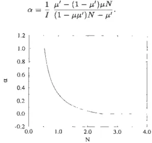
The steady state can be characterized equivalently by the rotation of the particle. The relevant dimensionless

variable is then a =

wjv.

The steady-state diagram in

the N - a space is shawn in Fig. 4. For a given value of the driving force, whatever the initial velocities, a is

attracted to a point on the steady-state diagram. In

phase 1, the steady-state value of a is equal to unity, while it is equal to zero in phase 3. ln phase 2, a de-creases with the driving force as

(11) 1.2 1.0 0.8 0.6 I:S 0.4 0.2 0.0 -0.2

o

.

o

1.0 2.0 3.0 4.0 N

FIG. 4. Steady state of the single-particle problem inN -a space, where a =

%

·

Ail forces and accelerations are

normal-ized ( see text). The steady state depends only on parameters

It can also be shown that the particular motion of the particle, for a given driving force, is the one that mini-mizes the dissipation.

In the equations of the problem, the particular value of unity for the coefficients of friction appears to play a key role. So far, we have tacitly assumed that the two coefficients of friction were smaller than unity. However, it is now straightforward to understand what happens when this is not the case. If J.L

<

1 and J.L1

_>

1, then the only steady state is phase 1: the particle can only roll on the plane. If J.L

>

1 and J.L1

_<

1, then it is phase 3 that dominates the steady state: the particle can only slide on the plane. In the case where both J.L and J.L' are greater than unity, no motion at ali is possible! The par-ticle simply sticks to the plane. It is easy to see that if the driving force N had a component downward, then the same situation would occur even for smaller values of the coefficients of friction. In this respect, unity has nothing special and reflects only the particular geome-try we consider here. In a long array of particles this same effect takes place when the coefficients of friction are greater than unity, and the applied force is screened by the particle in contact with the pushing block. This

observation suggests that in granular media, things will change radically when the interparticle coefficient of fric-tion is high ènough. In the forthcoming sections we will assume that the coefficients of friction are smaller than unity.

III. A ONE-DIMENSIONAL ARRAY OF PARTICLES

The study of the motion of a single particle provides us already with sorne insight into the question we address in the general case of a long array. How are the rotations of the particles organized in the steady state? How does the motion of the system depend on the applied force? Our aim is to propose a global description of the fric

-tional motion of this system as a result of the collective organization of rotations.

We have set up a computer program to simulate the motions of particles on a plane. The case of a single par-ticle (Sec. II) shows that the friction law is actually the most important ingredient of the problem. Our program prescribes the exact Coulomb law (with no regulariza-tion) at the particle-particle and particle-plane contacts. We are interested in the situation where each particle remains in contact with its neighbors, so that the whole system can be considered as a single abject. This require-ment is motivated by our purpose here to focus on the role played by the rotations in the translational motion of the array. Only if ali interparticle contacts are closed can the global translation be defined. Hence, the system we simulate is collision free and the relative velocities at

contact points are only tangential. Moreover, our system involves no cohesion force and no elasticity.

As we shall see later in this section, the close-contact condition is satisfied only for a limited region in the pa-rameter space. We add a second block to confine the array, where a constant force opposite to the direction of

motion is applied to the first particle of the array.

Al-though this new parameter is neither necessary nor suffi-dent to prevent particle-particle contacts from opening, it is, in general, a very useful control parame ter, espe-cially when the driving force is weak. So, the parameters are the following: J.L, J.L1

, and J.L11 are the coefficients of interparticle, plane-particle, and block-particle friction, respectively. The driving force NL, the confining force

No, and the number of particles L are the other param-eters, as shown in Fig. 5.

A. Governing equations

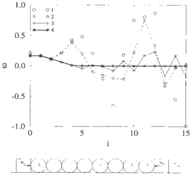
Figure 5 shows a scheme of the array with the sign conventions for forces used throughout this paper. With these conventions, the equations of dynamics for each particle i are written

T(i)- T(i- 1)

+

R(i) = 1, N(i)- N(i-1)

+

S(i)

=

T(i)

+

T(i-1)-S(i)

v,

Iw(i).

The boundary conditions are

N(L)

=

NL,

N(O) =No.

(12)

(13) There are 5L

+

1 variables to be determined, whereas we have only 3L equations given by dynamics. The remain-ing 2L

+

1 equations are prescribed by the contact law at the 2L

+

1 contact points.

In order to avoid any artifact in the solution of our equations, we would like to use the exact Coulomb law of friction. However, it is not straightforward to im-plement it in an algorithm, since, as shown in Fig. 2,

the (vr, T) should belong to a set of admissible values.

1.0 0.5 ·8 0.0 -0.5 -l.O 0 '"'"' 1 <)--~2 -1-1-3 *----*4 0 5 .o· .o o··· ~ i ,'\ 10 ' 1 1 ' ' _{~ '.} 15

.

FIG. 5. {a) An array of particles on a plane. (b) Forces exerted on the particle i and sign conventions.

A mathematical framework for handling such problems, known as nonsmooth analysis, has been developed [8].

In static equilibrium, where all the relative velocities are zero, Coulomb's law results indeed in an indeterminate state of forces (the so-called hyperstaticity of a sand

-pile at equilibrium). Nevertheless, in a dynamical system where the particles are moving and the states of contacts are permanently subject to change, the friction force on the vertical branch of Coulomb's law can be determined

in a unique way. We have shown this explicitly in the case of the single-particle problem. The main point is that one has to distinguish the contacts where the rela-tive tangential velocity remains equal to zero from those where this is not so. ln terms of the relative accelera-tions, we would say that there are two classes of contacts where the relative tangential velocity is zero: one where only the relative tangential velocity is equal to zero and one where both the relative tangential velocity and accel-eration are equal to zero. We shall caU them active

con-tacts and nonsliding contacts, respectively. Whenever a

contact is active, i.e., when v,. = 0, there are three differ-ent alternatives distinguished by the relative tangential acceleration ù,. at the contact.

(1)

v,.

=O. In this case, the contact is nonsliding. The friction force T has to be in Coulomb's limits [-J..LN,J.LN],

where N is the normal force at the contact. Here we have an equaiton and an inequality. When the equation

v,.

= 0

supplements the equations of dynamics, we get the values of T and N and we can check for the inequality. If the inequality is satisfied as well, then we have the solution.

If this is not so, we have to switch to one of the two other alternatives.

(2)

v,.

>

O. ln this case, the contact is sliding although it is active. So, we have to put T = - J,LN following the sign convention of Fig. 2. We supplement the equations of dynamics with the latter equation, from which we cal

-culate

v,.

among others, and we check for the inequality.

If the inequality is not satisfied, then we turn to another alternative.

(3)

v,.

<

O. This is the same as the second case except that the corresponding equation is T

=

J,LN.

In this way, Coulomb's law in its most general formu-lation takes the following form:

r

= 0 and TE [-J.LN, J..LN],

v,. = 0 => ~r

>

0 and T = -J,LN,

v,.

<

0 and T

=

J,LN, (14)

Vr

>

0=> T= -J..LN,

v,.

<

0=> T=J..LN.

ln order to solve the system of equations when a contact becomes active, the three alternative configurations are to be tried successively until the solution is found. Actu

-ally, there may be a great number of nonsliding contacts in a granular medium at the same time. Whenever a single contact becomes active, all the other nonsliding contacts are to be considered as weil. For p active con-tacts, this implies 3P possible configurations. Depending on the situation, different phenomena may take place. When a contact becomes active, it may become

nonslid-ing, but cause other nonsliding contacts to turn sliding at the same time; or it may simply turn out to be a sliding contact and force other nonsliding contacts to become sliding ones as well, and so on.

This basic image is too time consuming to be imple

-mented in an algorithm, since the number of possible con-figurations grows exponentially with the number of active contacts. An important ingredient of our computer pro-gram is a relaxation scheme that converges rapidly to the solution in the space of configurations. The method used is to start with an arbitrary configuration when, in the process of evolution of the system, sorne contact becomes active. Then, if the selected configuration is not the right solution, it is mapped onto the space of configurations in arder to build a new configuration to be tested. This iterative process converges very rapidly to the solution with the following mapping:

v,.

=

0 and T

<

-J.LN ----+ T

=

- J.LN,

v,.=

0 and T

>

+J.LN ----+ T = +J.LN,

(15)

T =-J..LN and Vr

<

0 ----+

v,.

=

0,

T

=

+J.LN and Vr

>

0 ----+

v,.= o.

This procedure has to be applied simultaneously to all active contacts.

The evolution of the system can be studied starting from a random initial state. The easiest way to generate initial conditions is to choose initial velocities in such a way that ali contacts are sliding. For a given value of the driving force NL, all accelerations and forces can then be determined. These values do not change unless sorne contact becomes active. Meanwhile, the motion of each particle is uniformly accelerated and the time fJh needed for sorne contact to become active is simply given by

. { . v,.(i)

fJh =mm fJh(t) = -v,.(i)' oh(i)

>

o

}

.

(16)

At this moment, a relative tangential velocity at sorne contact vanishes and new values of forces and acceler-ations are to be calculated. Since the states of sorne contacts change, the values of forces and accelerations undergo discontinuous changes. The motion is again uni

-formly accelerated. This event-driven process continues until the system achieves the steady state where at every contact the relative velocity and acceleration are of the same sign or both are zero. In the steady state, all forces and accelerations rem ain the same forever.

B. Numerical results

Our simulations show that, depending on the driv-ing force, three different regimes may occur. For small enough values of the driving force and for most initial conditions, sorne interparticle contact opens and the ar-ray separates in two or more identical arar-rays. On the other band, for large enough values of the driving force, sorne particle-plane contact may be lost and the geome-try of the array is modified because of the rising of one particle. ln between these two limits, all contacts are preserved. We consider only this intermediate regime,

ters are such that the steady-state value of Mis smaller than the particle-plane coefficient of friction.

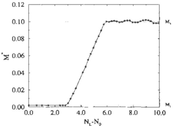
The global steady-state coefficient of friction M of the

array, although independent of the initial conditions,

dif-fers from the ordinary coefficient of friction in that it is a

function of the driving force. Figure 9 shows this

depen-dence for a system of 20 particles. M increases from zero

linearly with N L and satura tes to a value equal to the

particle-plane coefficient of friction. In other words, for

weak values of N L, the driving force is accelerating the

system less than it would if the particles were replaced

by a single block. Another effect of the driving force is

to regulate the internai organization of forces so as to

increase its frictional resistance. For weak enough values

of the driving force, the system is in phase 1. Dissipation

takes place only at interparticle contacts. In this regime,

M increases linearly with the driving force because, as

we shall see in the next section, in phase 1 all forces

scale with the driving force except for the normal force

on the plane. As the driving force increases, more and

more particles of phase 2 appear in the tail of phase 1

and hence the number of particles in phase 1 decreases.

Then, Mis no more linear in NL. Finally, when the

driv-ing force is high enough, phase 1 disappears completely

from the array so that ail particles are either in phase 2

or in phase 3. In this regime, M is simply equal to the

particle-plane coefficient of friction. Thus, the number of rolling particles indicates the capacity of the system to

increase its friction. Figure 10 shows the configuration of

rotations in the steady state of a system of 40 particles

for different values of the driving force. The connection

between the rotation modes and the global behavior of

the array in translation will be studied in more detail in

the next section.

IV. THEORETICAL ANALYSIS OF THE

STEADY STATE

In this section we will focus on the steady state and the

mechanisms leading to the spatial patterns of rotations.

These patterns provide the key to the global description

of the array as a single object in displacement.

0.12 0.10 0.08 ::E 0.06 0.04 0.02 0.00 0.0 2.0 4.0 6.0 8.0 10.0 NL

FIG. 9. Variation of the global coefficient of friction of an array of 20 particles as a function of the driving force. Pa-rameters are J.L = 0.01, J.L1

=

0.1, and No

=

0.05.

·8 0.20 r---~---~---, 0.15 0.10 0.05 0.00 -0.05 0 ---·-- - Nt.=4 N,..() ·---N,_-=8 - N,=IO . -·-·-· -·-·-· ·-·";-,.· .. ~·-·-.· ...

-·-·-

-·-.... t 10 20 30 40

FIG. 10. Angular accelerations of particles in an array of 40 particles for different values of the applied force. Here,

J.L = 0.01, J.L1

= 0.10, and No = O.

A. Different phases

The most interesting feature of the rotation patterns

is that pure phases of rotation come one after another

without mixing. This scheme suggests that as one goes

along the array, sorne quantitative changes in the state

of forces are followed by qualitative changes resulting in

quite different behaviors. Let us consider first the case

of rolling (phase 1).

Since ali of the particles in phase 1 are rolling in the

same direction, friction forces at interparticle contacts

are fully mobilized so that the equations of dynamics can

be supplemented in this case by

T(i) = -J.LN(i). (18)

Moreover, rolling implies

w(i)

=v.

(19)

From Eqs. (12), (18), and (19) we get the following

ex-pression for the friction force at particle-plane contacts:

) ( )

i 2J.L 1

+

I . 1

+ J.L

S(i)

=v-

- -

(No

+ --v

- -

,

1

+

J.L 2J.L 1 - J.L (20)

as well as the following limit on the value of the

particle-plane force:

- S(i)

<

J.L'(1

+

J.LV).

- 1

+

J.LJ.L' (21)

Equation (20) shows that the particle-plane friction is

mobilized progressively along the array and its direction

is opposite to that of the motion. The absolute value

of the friction force has an upper bound given by (21).

From (20) and (21) one gets the maximum number of

parti des in phase 1:

.

{1

(

1 1 - J.L ( . ')) t :::; L1 = 1

+

n - , v

+

J.L 2J.L 1 - J.LJ.L

(

1+1

.

)}/ (1+J.L)

- ln N0

+

~v ln 1 _ J.L , (22)

where L1 is the length of phase 1. So, the simple

mech-anism behind this phase is the progressive mobilization of the friction force at particle-plane contacts up to the maximum possible value of the friction force. Simulations in fact confirm this simple picture; see the functions S(i) and w(i) in Fig. 7 from the simulation of an array of 40 particles. The contacts of the particles coming after the particle i = L1 with the plane can no longer be

nonslid-ing and in phase 2, even if the particles continue rotatnonslid-ing in the same direction, all contacts are sliding contacts.

Now, let us consider the situation where all contacts are sliding contacts and all of the particles rotate in the positive direction (phase 2). The following equations are then to be used to supplement the equations of dynamics:

T(j) -11-N (j),

S(j) = -11-' R(j),

w(j)

>

o.

(23)

From these and the equations of dynamics we get the following expression for the angular accelerations:

lW ) = -. ( ') 211-(11-' +v) . J+ !1-(1

+

11-') . V

1 - 11-J-L' 1 - I-Ll-L'

+11-'(1 + 11-) -2 'N(. = 0)

1 - 11-/1-1 Il- J , (24) where j refers to the jth particle of phase 2 and N(j = 0)

is the normal interparticle force on the fust partricle in the phase. At the same time, we have

S(j)

=

_11-'(1

+

11-v).

1 - 11-11-' (25)

These equations show that the angular acceleration is de-creasing linearly with the particle number while the fric-tion force at the particle-plane contact remains constant. However, the positivity of the angular acceleration, which is a consistency condition, gives the maximum number of particles in the phase:

. <

L = _1_ [1

+

11-' v + 11-'(1 +11-)

J - 2 11-'

+

v 2

2!1--(1-

J-L~-L')N(j

=

o)],

(26)

where L2 is the length of phase 2. This simple mechanism behind phase 2 is illustrated in Fig. 7, where T(i) and

w (

i) are shown for a simulation of an arr a y of 40 partiel es. From the end of phase 2, the behavior changes again radically as the particles can no longer rotate consistently in the same direction.

Let us now consider phase 3, where the interparticle contacts can no longer be sliding. The equations to be used to supplement the equations of the dynamics are the following:

S(k) = - 11-' R(k),

w(k) = - w(k + 1) =w. (27) Assuming that the fust particle in this phase in contact with the last particle of phase 2 bas a negative rotation velocity, we immediately get the following expression for

the tangential interparticle force: T(k) = _[ T(k = 0)

+

-

11-'

+

-

lw]

2 2j.L1

(

~

_{1 - 1-L'}

)k

k lw 11-'

-(-1) - - - .

211-' 2 (28)

The interparticle friction force oscillates with a period of two particles and grows exponentially. We remark that this behavior of the interparticle friction force is only re -lated to the fact that the interparticle contacts here are nonsliding. Even in the case where

w

=

0, which is a particular case of phase 3, this oscillating behavior is ob-tained. ln the same way, we get the following expression for the normal interparticle force:

N(k) = N(k = 0) + k(v + 11-')

[ 11-'

lw]

+

11-' T(k = 0)

+ 2 +

₂11-, [ ( 1

+ ')

kl

x

1

-

-

1-:1

.

(29)

From Eqs. (28) and (29) and the boundary condition T(O) = - 11-N(O), it is easy to see that JT(k)l $ 11-N(k)

for all k. The length of phase 3 is thus not limited by the mobilization of the interparticle friction forces. However, sorne limit arises from the normal particle-plane force which, for consistency of the equations, bas to be posi-tive. The expression of the normal particle-plane force is the following: R(k) = 1

+

(-1)k

1

~

11-+

- -

2 [ T(k = 0)

+

!:!:__

+ __:::._

1

l']

1 - 11-' 2 211-' x [-1+ 11-']k-1 1 - 11-' (30)

The positivity of R(k) sets an upper limit on the length of phase 3: k $ L3 = 1 +

{ln [

1

~

11-' ( 1

+

:,

)

]

[ 1-L'

lw

] }

1 (

1

+

11-' ) - ln T(O)

+ 2

+

₂11-, ln 1 _ 11-' , (31)

where L₃ is the maximum length of the phase and T(O)

is to be replaced with the last particle in phase 2. The particle coming just after the particle L1

+ L

2

+

L3 will

rise as the reaction force on the plane vanishes.

What is the relation between

w

and

v

in phase 3? There are not enough equations to relate these two accel-erations. The answer is to be looked for in the boundary conditions. For the array to be stable (no contact open-ing), we should have L $ L1

+ L

2

+ L

3 . Suppose that

there is an even number of particles in phase 3 so that

the last particle is rotating in the positive direction. As

friction generally different from J.L, its angular accelera-tion is different from that of phase 3. Simulations show that if J,.L11

_<

_{J.L, then the angular acceleration of the last}

particle is greater than that of phase 3. In this case, the contact between the last particle of the array and the last

particle of phase 3 is sliding and we have the consistency condition T(k

=

L~ - 1)

=

-J,.LN(k

=

L~-1), where L'

is the length of phase 3. This gives the relation between

w

and

v.

As seen in Fig. 10,

w

decreases with the driving force, while

v

increases. Figure 11 shows the angular

ac-celerations of the particles in two simulations: one with

J.L11 = 0, the other with J.L11

>

J.L. ln this latter case, the rotations in phase 3 simply vanish.

B. Global dynamics

The global behavior of the array results from the juxta-position of the three rotation phases. By global behavior,

we mean the relation between the applied force NL- No,

as input to the system, and the acceleration

v,

which is

a global output. ln this section we will show that, as in the case of a single particle (Sec. II), this relation can be cast in the canonical form of the equation of frictional motion of a single black:

NL- No- F* = m*v, (32)

where m*, the effective inertia and F*, the effective fric-tion force on the plane, are funcfric-tions of the parameters and the applied force. Figure 12 shows

v

as a function of N L - No for an array of 20 particles. The inverse

of the slope at each point corresponds to the effective inertia for the corresponding value of the applied force, while the intersection with the axis of accelerations gives the effective friction force on the array. Three different

regimes can be distinguished.

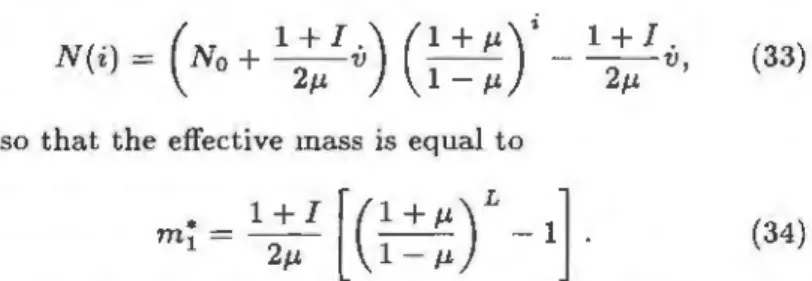
(1) From zero up to a critical value N' of the applied

force, the effective mass is constant. In this regime ali

particles are in phase 1. From Eqs. (12), {18), and (19) it can be shawn that the normal interparticle force in

phase 1 is given by ·9 0.05 0.00 <>-<> )1" =0.00 -~Ji".O.IS -0.05 ,__ _ _..._ _ _ ~ _ _ .__ _ __._ _ _ _, 0 2 4 6 8 10

FIG. 11. Angular accelerations of particles in an array of ten particles for two different values of the particle-block co-efficient of friction J.l-11• The other parameters are JI- = 0.1,

J.L1

=

0.2, No

=

0.1, and N L

=

2.8. 0.30 ·?0.20 0.10 0.00 V--~--__._ _ _ _._ _ _ _.__ 0.0 2.0 8.0 10.0

FIG. 12. Translational acceleration of an array of 20 parti-des as a function of the applied force N L - N0 . Parameters are J.L = 0.01, J.L1 = 0.1, and No= 0.05.

N( .) _ '1. -

(N

o

+

- - v 1 + I . ) ( - -1

+

J.L) i - -1

+

- l . v

2J,.L 1 - J.L 2J,.L ' (33)

so that the effective mass is equal to

m • ₁ =

~

[ (

1

+

J.L) L -

1]

2J,.L 1 - J.L (34)

Thus, the effective inertia in this regime can be rouch greater than the real mass

L

of the system. lt increases

rapidly with J.L and for small values of J.L, is at least 1 + I

times the real mass of the array.

From Eq. (33) we get also the following expression for the effective friction force:

(35)

ln Sec. III, we introduced a global coefficient of friction

M, which is the "total'' friction force F on the plane di-vided by the real mass L of the system. Since a global description implies analytically an effective inertia to be introduced, a description in terms of "effective" quanti

-ties is more consistent. Hence, we introduce the effective

renormalized coefficient of friction by

M* = F*.

m* (36)

We recall that the acceleration of gravity bas been set to 1. From Eqs. (34) and {35), the expression of M* in the regime of collective rolling is given by

(37) This is a simple expression in that it depends neither on the applied force nor on the number of particles. In this respect, M{ shows exactly ali the features of a Coulom-bian coefficient of friction.

The confining force No in this regime is a control

pa-rameter of M{. When No = 0, the effective coefficient of friction vanishes! The system is bence reduced to a black with no friction on the plane and an effective mass

greater than its real mass. This has interesting physical implications. For instance, since the effective inertia is greater than the real mass, the speed of sound through the system, due to a small elasticity at contact points, should be less by at least a factor of v'1

+

I than when rotations are absent. On the other hand, since the

fric-tion force for small values of 1-L is proportional to the number of particles L, a small change in the confining force is amplified by a factor L to give a much larger friction force.

(2) When the applied force is greater than N', the ef-fective mass begins to increase with the applied force. At the same time, the number of particles in phase 1 de-creases and there are more and more particles in phases 2

and 3. As long as there are particles in phase 1, the effec-tive mass continues to increase. From Eqs. (12) and (23),

it can be shown that the effective mass and coefficient of friction in phase 2 are given by

m• - 1 _L

2 - 1-J.<p.'

Mi

= 1-L' (38)

where Lis the number of particles in phase 2. In the same way, for phase 3, from Eqs. (12) and (27), we obtain

m3

= L,

M* ₃

=

_{,_}

u'

-~

_L

[(~)L

_{1- p.'}

-

1]

x (

-

~.LN(k

=

0)

+

~

+

J;,).

(39)

where Lis the length of phase 3. Here we have taken

w

to be an independent parameter which is related essentially on the particle-block coefficient of friction. The effective coefficient of friction in phase 3 is approximately equal to f.L1• The deviation from this value is of the order of I.L'3

when the angular acceleration is zero, and of the order of

f1,12 otherwise.

The effective inertia and coefficient of friction of the array can be calculated from those of the phases:

m • mi

+

m~

+

mj,

M*

=

Mimi+Mâmi_m.i+m;+m; +M;m;

(40) As the number of particles in phase 1 decreases, the ef-fective coefficient of friction increases and, at the same time, the effective inertia of the array tends to its real mass.

(3) For a certain value N" of the applied force, there

will be no particle in phase 1 and the relation between ac-celeration and applied force becomes linear again. In this regime, the effective mass is practically equal to the real mass of the system, except for small oscillations coming from phase 3. The effective coefficient of friction in this regime is equal to the particle-plane coefficient of fric-tion. Figures 13 and 14 display the variation of effective coefficient of friction and effective inertia as a function of the applied force for an array of 20 particles. N0 and f.L

are the control parameters of the first regime.

It can be seen from Fig. 13 that the necessary condition for observing the fust regime for any number of particles is given by a simple inequality:

0.12 ,--~--~---~--~---, 0.10 0.08 .::E 0.06 0.04 0.02 0.00 b==~!;::···-""-···.:::.~·-"-"····:;;;:··:;;;; .. ·-;:;;;·-·;;:;;"-·= = = = - '·:.::."''d"" M, 0.0 2.0 4.0 6.0 8.0 10.0 NL-NO

FIG. 13. Variation of the effective coefficient of friction as a function of the applied force for the system of Fig. 12.

Mt

=

2J.t/(l

+

I)No is the effective coefficient of friction in

phase 1. M3 = J.t1 is the mean value of the coefficient of friction in phases 2 and 3.

( 41)

When the confining force is small, the system is always in the fust regime for small enough values of the ap

-plied force. Collective rolling of particles should occur for example at the free surface of sandpiles. Therefore, physical effects due to this mode should be observable in real sandpiles.

V. CONCLUSION

We have introduced a simple one-dimensional model of particles where the interplay of the dynamics and the contact law (Coulomb's law of friction) leads to a well defined organization of the rotations of particles in the steady state. This self-organization has been studied nu-merically and analyzed in terms of a juxtaposition of "pure modes." The latter have been fully characterized analytically and their respective lengths have been com-puted. The agreement between the numerical simulations and the theoretical analysis is perfect.

40 ,--~--~---~---~--, 35 30 8 25 20 .... ----··---_,, .. ,_ .... ,_ . .,,- . ... --~ ... 15 L--~---~---~---~-~ 0.0 2.0 4.0 6.0 8.0 10.0

FIG. 14. Variation of the effective massas a function of the applied force for the system of Fig. 12.

The translational motion of the array on the plane in

the steady state can be described in terms of a global friction force, increasing with the external driving force. However, direct analysis shows that an effective inertia has to be introduced. This in turn requires an "effective" coefficient of friction to be defined, which is different from the "global" coefficient of friction in many respects.

Finally, let us stress the importance of length scales in-termediate between the particle size and the system size appearing in rotation modes and force patterns, which

may play a significant role in a continuum description of granular media. While this effect is limited here to

[1) W. Nowacki, in Theory of Micro-polar Elasticity {Springer,

Udine, 1972).

[2) J.-P. Bardet and J. Proubet, Géotechnique 41, 599 {1991).

[3] Chang and M. Lun, J. Eng. Mech. Div. ASCE 116, 2310 {1990).

[4] P. Evesque and D. Sornette, J. Mech. Behaviors Mater. 5, 261 {1994).

[5] L. M. Schwartz, D. L. Johnson, and S. Feng, Phys. Rev.

a one-dimensional geometry, we expect similar

qualita-tive effects in higher dimensionalities. A two-dimensional case is presently under study.

ACKNOWLEDGMENTS

It is a pleasure to acknowledge useful discussions with

D. Bideau, H. J. Herrmann, J. P. Troadec, and D.

Wolf. This work was supported by the Groupement de Recherche "Physique des Milieux Hétérogènes Com-plexes" of the CNRS.

Lett. 52, 831 {1984).

[6] H. M. Jaeger and S. Nagel, Science 255, 1523 (1992). [7] M. Jean, Mechanics of Geometrical Interfaces (Elsevier

Science Publishers, New York, 1994).

[8] M. Jean and J. J. Moreau, in Contact Mechanics, edited by A. Curnier, Proceedings of the Contact Mechanics

Inter-national Symposium, edited by A. Curnier (Presses