N-light-N : Read The Friendly Manual

(1)

N-light-N

Read The Friendly Manual

Mathias Seuret, Michele Alberti, and Marcus

Liwicki

Internal working paper no 16-02

August 2016

WORKING PAPER

DEPARTEMENT D’INFORMATIQUE DEPARTEMENT FÜR INFORMATIK Bd de Pérolles 90 CH-1700 Fribourg www.unifr.ch/informatics

(2)

N-light-N

Read The Friendly Manual

Mathias Seuret, Michele Alberti, and Marcus Liwicki

Document Image Voice Analysis group (Diva)

University of Fribourg

Boulevard de Perolles 90 - 1700 Fribourg - Switzerland

(3)

Abstract

This documentation wants to be a “user manual” for the N-light-N frame-work1. The goal is not only to introduce the framework but also to provide enough information such that one can start modifying and upgrading it after reading this document. This document is divided into five chapters.

The main purpose of Chapter 1 is to introduce into our notation and for-mulation. It refers to further literature for deeper introductions into the theory. Chapter 2 gives quick-start information allowing to start using the framework in an extremely short time. Chapter 3 provides an overview of the framework’s architecture. Interactions among different entities are ex-plained and the main work flow is provided. Chapter 4 explains how to write a custom XML script for the framework. Proper usage of all imple-mented commands is described. Finally, Chapter 6 explains how to extend the framework by creating your own script commands, layers (encoder/de-coder), and autoencoders. Having read both Chapters 3 and 6 before start-ing to extend the framework is extremely recommended.

As the framework will evolve, this documentation should be kept up-to-date2.

1_{Available at: https://github.com/seuretm/N-light-N} 2

The most recent version can be found at

(4)

Acknowledgement

The happy developers of N-light-N would like to thank for their help, col-laboration, and feedback the following persons:

• Ingold, Rolf • Chen, Kai • Dias, Emanuele • Fischer, Andreas • Garz, Angelika • Oener, Volkan • Pastor, Joan • Sayadi, Karim • Simistira, Fotini • Sittampalam, Arun • Wei, Hao

This work was funded by the Swiss National Foundation (SNF) project HisDoc 2.0 with the grant number: 205120 150173.

(5)

5.2.2 Creating an Scae . . . 59 5.2.3 Training Scaes . . . 60 5.2.4 Extracting Features . . . 61 5.3 Classifiers . . . 62 5.3.1 FFCNN . . . 62 5.3.2 AEClassifier . . . 63 5.3.3 CCNN . . . 64 5.4 Training a Classifier . . . 64 5.5 Classification . . . 66 5.5.1 Advices . . . 67 6 Framework Upgrade 69 6.1 Creating your Own XML Command . . . 69

6.2 Creating your Own Layer . . . 73

6.3 Creating your Own Autoencoder . . . 75

6.4 Creating your Own Classifier . . . 76

(8)

Foreword

The foundations of neural networks are surprisingly old, as the first artificial neural networks date from the 1940s with the development of the McCulloch-Pitts neuron [1, 2, 3]. Since then, they have been used in many domains, including speech recognition [4], pattern recognition [5], stock market pre-diction [6], ... Decades of increasingly active research in this field have shown that artificial neural networks have a huge potential, and also that there is still much to learn.

Novel training methods and faster computers now allow to train and use neural networks which are much larger than it was feasible in the past. The term “deep learning” refers to the use of neural networks to learn data representation with different levels of abstraction, which can then be used for machine learning purpose.

Many libraries and deep learning frameworks are being used with increas-ing success in many fields. Accordincreas-ingly to Bahrampour et al. [7], the most frequently used ones are Caffe [8], Theano [9], Torch7 [10], TensorFlow [11], and deeplearning4j3. These libraries allow for efficient training of deep neu-ral networks with high paneu-rallelization and implementation on graphic cards, making them very useful, especially for image processing.

However, such optimizations have a two-fold cost for research and analysis. First, the performance optimization are obstacles for adaptability by non-experts, as high programming skills are required. Second, these optimiza-tions decrease the users’ analysis capabilities, and thus generate difficulties for a deeper understanding of the networks.

Thus, there is a gap that N-light-N aims to fill, as highly-adaptable frame-work for Convolutional Neural Netframe-works (Cnn) allowing not only deep mod-ifications with minimal effort, but also investigations on the inner working of the networks with ease. For this purpose, N-light-N follows a simplicity principle: base components that any user might some day want to modify should be kept as simple as possible, even if speed has sometimes to be sacrificed. Thus, barriers to entry for researchers are kept very low. It is

3

(9)

the authors’ hope that N-ligne-N will lead to exciting discoveries about deep learning.

A more scientific presentation of N-light-N together with experimental vali-dation and analysis is presented in [12]. This framework has also been used in published research on historical document analysis [13, 14, 15], historical document images clustering [16], feature selection [17], and for Arabic text detection in video frames [18]. Ongoing research is being done on novel meth-ods for Autoencoder (AE) training, central multilayer features usage [19], document graph [20] edge labelling, deeper understanding of historical doc-ument image clustering, and novel kinds of neuron-like units.

(10)

Chapter 1 Theoretical Foundations

This chapter is a refresh for those who are already familiar with the topics of machine learning, autoencoders and neural networks. Shall this not be the case, you can read this as quick introduction but do not think that this short theory somehow replace a proper study of the subject. For getting a solid knowledge about deep learning, we recommend the following books. As introduction to neural networks, we recommend reading “Neural networks: a systematic introduction” [2]. A thorough historical survey of deep learn-ing, “Deep Learning in Neural Networks: An Overview” [3], provides both information about past and current research on neural networks. Finally, “Deep Learning” [21] is a course covering most, if not all, aspects modern deep learning.

Stacked Convolutional Autoencoders (Scaes) are based on three principles which will be described in the following sections: autoencoding, convolving and stacking.

1.1 Autoencoding

AEs are mostly used for computing feature vectors which can then be used for machine learning purpose. They are composed of two functions:

~

y = E (~x) and ~x0= D (~y) such that ~x ≈ ~x0.

The idea is to take an input vector ~x, encode it into ~y and then decode it again to ~x0 expecting to have only little differences with the initial input ~x. The encoding and decoding functions are learned during the training of the AE, where the training error is the difference between ~x and ~x0.

(11)

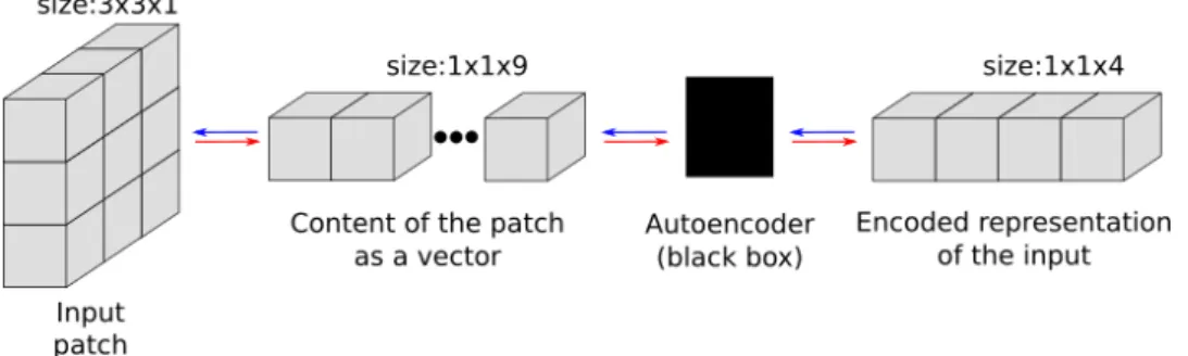
science. Figure 1.1 shows an AE taking as input a 3×3 pixels patch from a one-channel image and outputs a four-dimension vector.

Figure 1.1: An autoencoder with his inputs and outputs. The arrows correspond to the data flow. Red arrows correspond to encoding the inputs, and blue arrows to decoding the outputs.

There are many different kinds of AE1, and while we mostly focus on the neural network terminology for simplicity reasons, you can consider an au-toencoder to be “anything that can encode and decode data”.

1.1.1 Dimension of the Encoded Representation ~y

The dimension of the encoded representation ~y is not fixed as it depends on the architecture of the AE itself. We have the three cases:

|~y| < |~x| → the encoded output is a is a compressed representation of ~x. This is particularly useful because if ~x ≈ ~x0 holds, it means as the input can be reconstructed with a fair accuracy with less values, some unnecessary information is discarded. In other words, all information lost during dimensionality reduction are not needed and thus we have that ~y is the “essence” of ~x. In computer science we often call this “essence”: features.

|~y| = |~x| → the encoded output is the identity ~x. This is in general not used as the AE could just learn the identity function and would therefore not lead to useful features.

|~y| > |~x| → might be done when training the AE to generate a sparse2

representation of ~x.

1

For now, the software supports the following kinds of AE: autoencoding neural net-works, denoising autoencoders, principal component analysis, and a naive implementation of restricted Boltzmann Machines.

(12)

1.2 Stacking

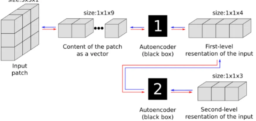
Stacking AEs literally means creating a stack with them. This means that the output of a first AE is used as input for a second (and different) AE. It can be done sequentially, typically with increasing compression rate such that |~yi| > |~yi+1|, where ~yi is the output of the i-th layer of the stack, as

illustrated in Figure 1.2.

Figure 1.2: Stacked autoencoders. When encoding data, AE-1 has to be computed first, while when decoding data, AE-2 comes first.

1.3 Convolving

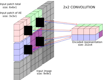
AEs can be convolved, i.e., it is possible to compute the output of a single AE at different locations in a neighborhood (typically in a grid-like pattern, often with overlapping patches). The outputs of the AE are collected in a 3D array called encoded representation, as shown in Figure 1.3. In this document, we call convolution width and convolution height the number of times the AE is applied horizontally and vertically (2 and 2 in Figure 1.3).

(13)

Figure 1.3: 2 × 2 Convolution of an AE with input 3 × 3, resulting in a 2 × 2 × 4 array. Note that the gray parts in the image are disregarded in this example.

As seen in Figure 1.3, the area covered by the convolution does not nec-essarily have the same size has the input image. For example, in case of pixel-labelling tasks, it is usually sufficient if the pixels being classified as well as some neighborhood are covered by the convolution. However, when classifying the whole content of an image, then the whole image has to be used for input.

Take note however that using Scaes on high-resolution images can be very time-consuming. The computational cost of a neural network is roughly linearly proportional to its number of inputs multiplied by its number of outputs. Convolutional Neural Networks (Cnn) or Scae are less expensive, as a single output of a layer is not connected to all inputs of that layer, but nevertheless the computational cost can be high when large areas are covered.

1.3.1 Convolution Offset

We call convolution offset the space between two AEs in a convolution. The offset is defined with two numbers H and V which specify how many pixels should be left horizontally and vertically between two input patches of the AE. In the literature, this is also often called “stride”. The reference point

(14)

for the input patch of an AE is the top left corner, as ilustrated in Figure 1.4.

Figure 1.4: Examples of horizontal convolution using an AE with a 3 × 3 pixels input patch. The red and green correspond to two locations, A and B, of the AE in the convolution. The full color squares represent the reference point of the AE in location A or B. In the left case the offset is 4 pixels, leading to a distance of 1 pixel between two AE locations. In the right case the offset of 2 pixels leads to an overlap of 1 pixel on the 3rd column.

What is illustrated in Figure 1.4 applies also for the vertical axis. There are two special cases. First, if the offset value is equal to the input dimensions of the AEs, then there is no overlapping and not distance between the input patches (like in Figure 1.3). Second, if the offset value is 0 it means the AE will be applied always on the same place: this is a mistake which should lead the library to raise an exception.

1.4 Stacking & Convolving Autoencoders

The main idea of this framework is to convolve and stack AEs, as depicted in Figure 1.5, in order to get different levels of features which can then be used for machine learning purposes. The main questions for setting up an Scae are:

• Which input patch size is optimal for each layer?

• How many features should there be in the different layers? • Which convolution width & height should be used?

• Which convolution horizontal & vertical offsets should be chosen? There seem to be no magical formula for answering accurately to these questions, thus to the best authors’ knowledge, only experimentation can really do this. Take note that as the weights of the AEs are initialised

(15)

randomly, small accuracy differences might not be significant unless you run the tests several times. In such a case, we recommend to use the t-test from DivaServices3 [22] which allows to run significance tests in an extremely simple way.

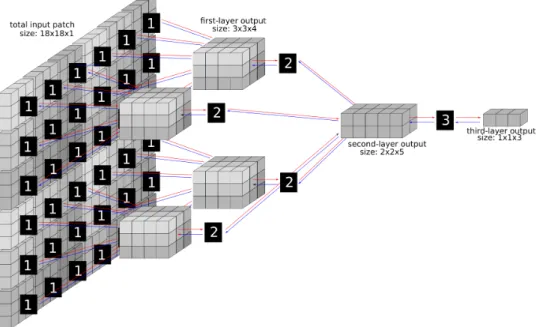
Figure 1.5: A stacked convolution autoencoder composed of two layers.

1.4.1 Determining Sizes

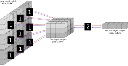
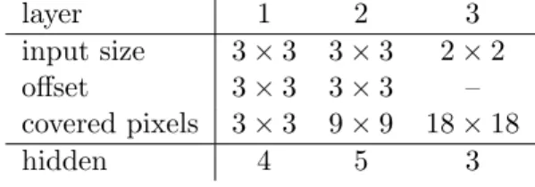
When building a stack of AEs, each layer corresponds to the convolution of an AE. The top layer however is a 1 × 1 convolution, i.e., its AE is computed at only one location, as it can be seen in Figures 1.5 and 1.6. Assuming that we have a N -layers stack, then, for adding the N + 1-th layer the size of the convolution in layer N has to be increased because it must have an output of the same dimension as the input of the (N + 1)-th layer. The effect of resizing the size of the N -th layer is that the (N − 1)-th must also be resized, and so on for all layers. For this reason, adding a layer to an Scae might have a huge impact on its architecture. While users do not have to implement this backward size selection themselves, it is very important to understand it well when designing new architectures.

Figures 1.5 and 1.6 depict the convolution resizing. For simplicity reasons, offsets of the same size as the inputs are used in order to avoid overlapping. The first layer AE takes as input 3 × 3 pixels and outputs 4 values. The second convolution takes 3×3×4 values as input, thus when adding a second layer the first layer has to be convolved 3 × 3 times as shown in Figure 1.5. The third layer, as depicted in Figure 1.6 requires an input of 2×2×5 values.

3

(16)

Table 1.1: Definition of Scaes in Figures 1.5 and 1.6. While the input size corresponds to only one layer, the number of pixels covered by an AE depends also on the previous layers.

layer 1 2 3

input size 3 × 3 3 × 3 2 × 2 offset 3 × 3 3 × 3 – covered pixels 3 × 3 9 × 9 18 × 18

hidden 4 5 3

This means that the second layer must be convolved 2 × 2 times. The second layer then requires 6 × 6 × 4 inputs, which is obtained by convolving 6 × 6 the first layer.

Convolution sizes and offsets for a convolution layer are always based on its input. In Figure 1.5, the second layer has an input size of 3 × 3, which corresponds to having a 3 × 3 convolution in the first layer, and not to pixels in the image. Table 1.1 shows the difference between layer input size and pixels covered by the Scae shown in Figures 1.5 and 1.6.

1.4.2 Training Stacked Autoencoders

Training a deep neural network can be computationally expensive. Although recent methods have been shown to lead to little or no vanishing gradient, computing new weights for a full network can be time-consuming. To tackle this issue, Scaes are trained layer by layer during their construction. Before adding a new layer to an Scae, its (current) top layer is trained to encode and decode its input with little error. Already-trained layers are not trained anymore.

1.5 Classification

The features learned by an Scae correspond to the output of the top-layer AE. Three options are possible:

• They can be extracted and given to an external classifier (e.g., an Support Vector Machine (Svm)),

• Classification layers can be added on top of the Scae, turning it into a classifier.

• The features at the center of each Cae of the Scae can be concate-nated and given to an external classifier.

(17)

Figure 1.6: A stacked convolutional autoencoder composed of three lay-ers. Note that it was obtained by adding a layer to the Scae depicted in Figure 1.5.

The first option is closely related to methods based on hard-coded features extraction followed by classification. An example about how to do this is given in Section 2.2.

The second option is more interesting, as it allows to backpropagate classifi-cation errors not only through classificlassifi-cation layers, but also through feature-extraction layers in order to fine-tune the features for a classification task. The third option is a novel approach existing to our best knowledge only in N-light-N.

(18)

Chapter 2 Quick Start

This chapter contains the minimal information for using the framework as it is. More details about its component or its use are provided in the other chapters. We will first present how to train a Cae, then how to compute features from images using the Cae from a Java application.

2.1 Training a Convolutional Autoencoder (

Cae)

The compiled jar file is a standard Java application, which does not require anything exotic to be installed on your computer, so you can just start it from the command-line:

1 java -Xmx8G -jar gae.jar my-training-script.xml

The -Xmx8G option tells the virtual machine that it can use up to 4 GB of memory. Depending on the task, you might want to increase or decrease this. When the memory is not or barely sufficient, then Java’s garbage collector will use a lot of CPU power trying to free some memory – it is usually better to allow the use of more memory than necessary.

The -jar option with parameter gae.jar, tells the virtual machine which jar file should be executed.

Finally, the my-script.xml indicates which script should be executed. Some sample scripts are provided with N-light-N which you can use, and adapt if needed.

Please make sure that both the path of the jar and the one of the script are correct before launching the program. Note that you should avoid using absolute paths if possible.

(19)

2.2 Extracting Features

Once you have created and trained a Cae, extracting features from an image is a simple task which you can easily do from a Java application. You simply have to:

1. Load the Cae, 2. Load the image,

3. Let the Cae know where it should input data, 4. And ask it to compute a feature vector.

These 4 tasks correspond to the 4 following lines of Java code.

1 SCAE myScae = SCAE.load("scae.ae");

2 DataBlock inImg = DataBlock.dataBlockFromImage("input.png"); 3 myScae.centerInput(inImg, centerX, centerY);

4 float[] features = scae.forward();

This feature vector can then be used for machine learning purposes. Take note that the array returned by the forward() method is allocated only once – if you want to store several feature vectors you will have to clone it.

2.3 The OSX Special Case

By default, Mac OSX seems to use the 1.6 version of Java, which dates from 20051. The framework requires Java 1.8 (or more recent), therefore you might have to install the most recent version of Java and set your IDE/OS to use it. Some users have even indicated that installing Java 1.8 is not sufficient – a manual uninstallation of Java 1.6 could potentially be required.

(20)

Chapter 3 Framework Architecture

This chapter provides an overview of the framework’s architecture. Inter-actions among different entities are explained and a brief description of the main work flow is provided. If you intend to work on the framework, i.e., to extend or modify it (see chapter 6), you will need a very good knowledge about all of this.

3.1 Parsing Scripts

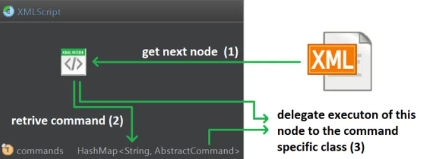
The class responsible parsing scripts and executing them XMLScript.java. When the framework is launched as stand-alone application, an XMLScript object is created and a map between command names and their implemen-tation is generated. Then, the XML script is loaded and parsed. Invalid XMLs (e.g., if closing tags are missing) will be rejected at this point. Then the content of the script is processed as shown in Figure 3.1 and described below:

(1) The children of the XML’s root element are processed in the same se-quence as they appear in the script.

(2) Commands matching the child’s names are retrieved from the map – if none is found then an error will be raised and the application will close. (3) The command then receives the tag as parameter so that it has access

(21)

Figure 3.1: Command execution procedure.

3.1.1 XMLScript

This class is the core for parsing the XML. As mentioned in Section 3.1, it contains a map linking all command names to the corresponding command objects. These objects also get a reference to the XMLScript object in order to be able to access to the resources, e.g., datasets or Scaes.

Each resource is is stored in a map and can be retrieved with its ID. The list of resources and information which the different commands might need is given below.

1. Image.Colorspace colorspace:

stores which color space is being used by the script. Commands must take this into account where needed.

2. Map<String, Dataset> datasets:

in lists of DataBlocks which can be used for training purposes. 3. Map<String, NoisyDataset> noisyDataSets:

special datasets storing not one DataBlock per image but two – one clean and one noisy version.

4. Map<String, SCAE> scae:

stores the Scae currently in memory. 5. Map<String, Classifier> classifiers:

stores the different classifiers currently in memory.

When creating new commands, it is mandatory to take the colorspace into account, even if not needed for the current experiment. One never knows what will happen next.

New commands must be added in the constructor of XMLScript following the same procedure as for the other ones.

(22)

3.1.2 AbstractCommand

All commands must inherit from AbstractCommand. This class allows not only to add new commands to the script, regardless of their nature, with minimum effort. It also provides some methods to extract and process data from XML elements. When implementing a new command, additionally to having to pass the reference to the XMLScript reference to the constructor (hint: think about the super keyword), two methods have to be imple-mented:

execute(Element)

responsible for carrying out the functionality the command provides. Here is where all the magic of the framework happens. The XMLScript object will call this passing the fetched node as parameter.

tagName()

returns the name of the command. This name must be a string which will perfectly match the name of the corresponding tag in the XML script. Names must respect general XML tag naming rules. Additionally, in or-der to keep the command names consistent, they should follow the form word1-word2-..., without capital letters. For instance command is is named load-dataset.

3.2 Data Structure

The whole framework works with the data structure of DataBlock. These blocks of of data are used as input for the neural networks, between layers and as output for neural networks. Users of the framework will have to deal with DataBlocks – fortunately they are very easy to use.

The following subsections present the DataBlock class, and its subclass BiDataBlock.

3.2.1 DataBlock

The DataBlock is an object which “simply” stores a 3D matrix of floats. Images can also be seen as 3D data, as they have a width, an height, and a given number of channels (e.g., 1 for grayscale images or 4 for CMYK images). The size of these dimensions is not fixed, i.e., the width, height and depth can have any value greater than 0 – as long as there is enough available memory.

The output of a convolution can be stored as an A × B × C DataBlock, where A is its width, B its height and C its depth, or number of channels.

(23)

The output of a single AE can be stored as an 1 × 1 × C DataBlock. This is well illustrated in Figure 1.5.

The framework uses DataBlocks instead of standard 3D arrays of floats in order to provide additional functionalities, including loading and saving DataBlocks, extracting areas from them into 1D float arrays, and “pasting” data into them with overlapping.

In the following parts of this section, we will present how to read and write data in a DataBlock. In Creating & Loading DataBlocks, the DataBlock constructors are presented. In Data Access, methods which are simple but should be sufficient for almost all uses are presented. Unless you need to modify deeply the framework, knowing these I/O methods is probably suffi-cient. In Non-Image Data, how to load custom data is explained. This might be very useful if you do not intend to work on image data. In Extracting & Pasting Patches, some additional methods to transform DataBlock patches to and from float arrays. And finally, in Weighted Paste, we explain how to cope with overlapping data, i.e., how to take into account that overlap-ping in convolutions can lead to a single value to be constructed from two different sources.

Creating & Loading DataBlocks DataBlocks has several constructors:

Listing 3.1: DataBlock constructors

1 public DataBlock(int width, int height, int depth) 2 public DataBlock(Image src)

3 public DataBlock(BufferedImage src)

4 public DataBlock(String fName) throws IOException

The first, and most generic constructor, allows to create a DataBlock with given dimensions. Should the user want to work on 1D or 2D data, some dimensions of the DataBlock can be set to 1. When storing individual samples in DataBlocks, we would recommend for performance issues to set the width to 1 when dealing with 2D data, and both the width and the height to 1 when dealing with 1D data.

Data Access

The dimensions of a DataBlock can be accessed with the following methods: Listing 3.2: Access to DataBlock dimensions

(24)

2 public int getHeight() 3 public int getDepth()

It is possible to access to single values in a DataBlock. The coordinates of a value are first indicated with the depth (corresponding to a color channel when the DataBlock contains an image, and to a feature when it is the output of an AE), and then x and y coordinates:

Listing 3.3: Access to a single value

1 public float getValue(int channel, int x, int y)

2 public void setValue(int channel, int x, int y, float v)

It is also possible to directly access to all channels corresponding to a given set of coordinates using float arrays. The following two accessors do not work “by copy” – the array returned by getValues is the one actually stored in the DataBlock. Also the array passed as parameter of setValues will replace the one stored in the DataBlock.

Listing 3.4: Access to all channels at a given location

1 public float[] getValues(int x, int y)

2 public void setValues(int x, int y, float[] z)

Non-Image Data

DataBlocks have some constructors to load image data. The XML scripts allowing to train networks such data, and if you intend to use different kinds of data as input for neural networks, you will have to implement a subclass of DataBlocks. For this, it is highly recommended to read Chapter 5 and, depending on what you intend to do, also Chapter 6.

As indicated in Section 3.2.1, DataBlocks consist in a 3D array of floats, so any data that fits in such an array can be loaded into a DataBlock.

If you have 2D data (similar to a grayscale image), then it is more efficient to project this data along the height and depth axes of the DataBlock. Let us assume that you have a function F (x, y) that returns the value of your data at coordinates (x, y), and that your data has a size of w × h. This could be done, e.g., by reading from a file. Then, you can load this into a DataBlock in this way:

Listing 3.5: Loading 2D data into a DataBlock

1 DataBlock db = new DataBlock(1, h, w); 2 for (int x=0; x<w; x++) {

(25)

4 db.setValue(x, y, 0, F(x,y)); 5 }

6 }

For 1D data, the values should be projected along the depth axe of the DataBlock. Assuming that you have a function F (x) that returns the x-th value of your data, and that your data is composed of w values, then you can load it into a DataBlock in the following way:

Listing 3.6: Loading 1D data into a DataBlock

1 DataBlock db = new DataBlock(1, 1, w); 2 for (int x=0; x<w; x++) {

3 db.setValue(x, 0, 0, F(x)); 4 }

This second case is probably the most likely to happen, as useful feature vectors extracted from data are sometimes already available, or when data of inconsistent size has to be mapped to a fixed-size space. For example, currently experiments are being made on classifying edges of graphs that represent the structure of document pages [20]. For classification with N-light-N, we compute a fixed-length vectorial representation of an edge that captures the structure of its local neighborhood (subgraph). Hence, a stan-dard AEs can be used.

Extracting & Pasting Patches

Scaes take as input patches in DataBlocks. A patch correspond to the values of all channels in a rectangular area of a DataBlock. For simplifying read/write accesses to patches from layers composing Scaes, the DataBlock class offers several useful methods.

Listing 3.7: Extracting a patch from a DataBlock

1 public void patchToArray( 2 float[] arr, 3 int posX, 4 int posY, 5 int w, 6 int h 7 )

8 public float[] patchToArray( 9 int posX,

10 int posY, 11 int w, 12 int h

(26)

13 )

The first version of patchToArray puts values from a patch starting at coordinates (posX, posY) and of size w×h into the (already-existing) array arr. The array must have a size of w×h×d, where d is the depth of the DataBlock.

The second version of patchToArray works in a similar way, but allocates the returned array and returns the result. It might be slower, but does not require to have an already-existing array.

The reverse operation, i.e., copying an array to a patch, can be done with the following method:

Listing 3.8: Extracting a patch from a DataBlock

1 public void arrayToPatch( 2 float[] arr, 3 int posX, 4 int posY, 5 int w, 6 int h 7 )

where the values in the array arr are copied in a w×h×d patch, where d is the depth of the DataBlock.

Note that the layers composing an AE (see Section 3.3.1) work with float arrays extracted by the patchToArray method. This extraction is done by the AEs (see Section 3.3).

Weighted Paste

The convolutions in Scaes might have some overlapping, which means an input value might be used more than one time. This also means that when decoding data, an Scae might transmit several values to the same coordi-nates of a DataBlock. The solution to deal with this is to accumulate these values, count for each location of the DataBlock how many values were ac-cumulated, and later divide the values by this count in order to get their mean. This count, which we call weight, is stored as floats which are shared for all channels of the DataBlock.

Using weighted paste and normalizing data, i.e., dividing values by the cor-responding weights, can be done with the following methods:

Listing 3.9: Pasting with weight

(27)

2 public void weightedPaste( 3 float[] arr, 4 int from, 5 int x, 6 int y 7 )

8 public void weightedPatchPaste( 9 float[] arr, 10 int posX, 11 int posY, 12 int width, 13 int height 14 )

15 public void normalizeWeights() 16 public void clear()

The first weightedPaste pastes a DataBlock into the target; this source DataBlock can be at most as big as the target. The second method pastes at a given location an array which length must be equal to the depth of the DataBlock. The third method pastes an array onto a patch – the length of this array must be equal to the number of values in the patch.

The normalizeWeights method divides all values by the corresponding weights, and sets all weights to 1. Finally, the clear method can be used to set all values and weights of a DataBlock to 0. This last method should always be called before starting to paste data with weights.

BiDataBlock

The BiDataBlock.java is an extension of DataBlock.java. The difference is that instead of a 3D matrix of floats, the data is stored in a BufferedImage (hence the name: BufferedImage DataBlock). The advantage of using this instead of a normal DataBlock is that it occupies less space in memory and is loaded faster. The drawback is that is it slower when being used, as RGB codes have to be turned into floats. It is possible to write float values in a BiDatablock with the different accessors, however these floats will be approximated as only 256 different values can be stored.

3.2.2 Dataset

Datasets are collections of DataBlocks. They are used by XML scripts, but can also be used outside of it. They implement the generic interface Collection<DataBlock>. Data is shuffled every time the iterator

(28)

me-thod is called, so iterating several times on a Dataset will not be done in the same sequence.

NoisyDataset

It is possible for a Dataset to contain two versions of each sample, one clean and one noisy. They can be used for training Denoising Autoencoders (Daes).

3.3 Autoencoder Building Blocks

Autoencoders (AEs) are the core of the framework. They are the building block for Scaes, which are then used for building classifiers.

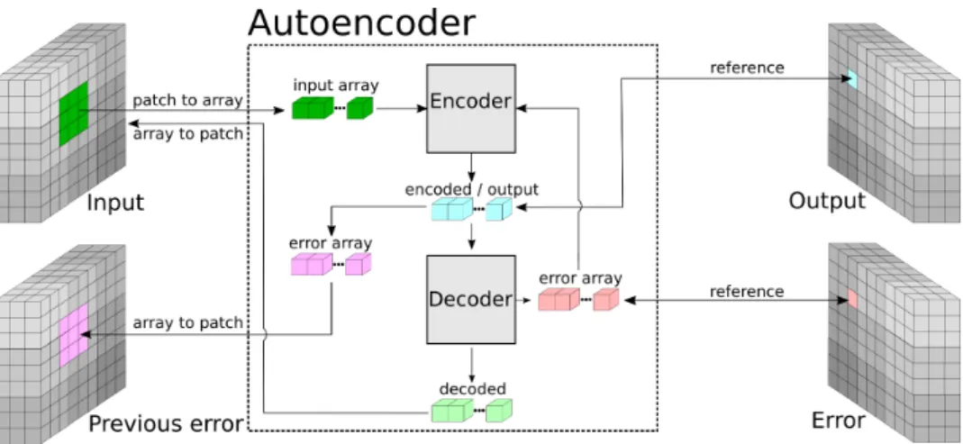
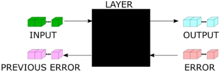
In this framework, AEs act as an interface between the high level entities (such as Scaes, classifiers) and the low level layers. The AE stores references to four DataBlocks : input, output, previous error and error, which are detailed below.

INPUT this is a reference to the input DataBlock. For the first layer this usually corresponds to an input image (which has typically a depth of 1 or 3, depending on whether the image is in grayscale or in color). For the other layers, the input corresponds to the output DataBlock of the previous layer and has depth equal to the number of features generated by the previous layer. The AE takes an input patch which might be smaller than its input DataBlock, and stores the coordinates of the top left corner of this input patch, as well as its width, height and depth. These coordinates (x,y of the top left corner) are the same for the previous error datablock, but are different for output and error.

OUTPUT this is a reference to the output DataBlock. If the AE is not convoluted this DataBlock has size 1 × 1 × n, where n is the number of outputs of the AE’s encoder. Otherwise, the next layer of the Scae determines the size of this DataBlock, as the input patch size of the next layer specifies how many times the current layer has to be convoluted. See Section 1 for more details. The depth of the output DataBlock corresponds to the number of outputs of the encoding layer of the AE; for each position in the convolution of the Scae corresponds a position in the output DataBlock. Thus, the encoding-layer requires only a reference to the corresponding 1D float array within the output DataBlock.

(29)

Figure 3.2: Data flow in an autoencoder. Note that input,output, previous error and error are Datablocks. The size (especially the depth) of the DataBlocks on the left of the figure might differ from the size of the ones on the right.

ERROR this is a reference to a DataBlock storing the error of the AE, rel-atively its encoding layer. When trained for encoding and decod-ing, or when trained for classification purposes, errors are back-propagated to the encoding-layer of the AE. These errors are stored in this DataBlock. The error DataBlock has the same size as the output one; when trained, the AEs read their error in this DataBlock at the same coordinates as they write in the output DataBlock.

PREVIOUS ERROR this is a reference to the error DataBlock of the previous layer of the Scae or classifier. For the first layer, this reference is null, thus accessing to this DataBlock should be done carefully. This DataBlock is used when backpropagating classifi-cation errors.

As we can see in figure 3.2 an AE is composed of two main parts: an encoder and a decoder. These two objects implements Layer the interface, which is detailed in Section 3.3.1, or extend the AbstractLayer class which already provides the implementation of some methods defined in the interface. The encoder and decoder of an AE do not necessarily have to be of the same class. This opens the possibility to create different kinds of AEs by simply providing them different kind of layers.

The abstract class AutoEncoder provides the basic functionalities for a nor-mal behaving AE (meant as the typical definition found on books and

(30)

de-scribed in Chapter 1). The AutoEncoder itself is used for managing its two layers by connecting them together correctly, managing inputs and outputs, and delegating calls of encode and decode methods, so the encoding itself is not implemented in the AutoEncoder class.

The concrete class StandardAutoEncoder implements AutoEncoder and provides constructors allowing to select the Layers by specifying their class name. The list of existing layers is given in Section 3.4.1.

For creating different kinds of AE which do not follow the standard encode-decode methodology, please refer to section 6.3 of chapter 6.

3.3.1 Layers

The two layers contained by an AutoEncoder must implement the Layer interface. As shown in Figure 3.3, all inputs and outputs are arrays of floats and not Datablock. Subclasses of AutoEncoder have to provide these ar-rays correctly to the different Layers, which means that when implementing a new kind of Layer it is not necessary to care about complicated data structures.

Figure 3.3: Interface of a layer. Notice how all inputs and outputs are array of floats and not Datablock, which means creating new layers does not require dealing with complex data.

The following methods below are present in the Layer interface. While there seem to be a frightening lot of them1, most are only accessors which are extremely easy and fast to implement and in most cases the abstract class AbstractLayer can be used (see Section 3.3.1).

In any case, the overhead of implementing this interface compared to the implementation of the encoding or decoding method can be considered as negligible. Listing 3.10 gives the list of the most important methods.

Listing 3.10: Some important methods from the Layer interface

1 void setInputArray(float[] inputArray); 2 void setOutputArray(float[] inputArray);

(31)

3 void setError(float[] error); 4 float[] getError();

5 void setPreviousError(float[] prevError); 6 void compute();

7 void setExpected(int pos, float expectedValue); 8 float backPropagate();

9 float learn(); 10 Layer clone();

These methods are described below:

setInputArray Indicates to the Layer from which array data will be read. Note that it might be called once or several times, so any class implementing the Layer interface should keep a copy of this reference.

setOutputArray Indicates to the Layer to which array it should write data. Note that it might be called once or several times, so any class implementing the Layer interface should keep a copy of this reference.

setError Indicates to the Layer where it will have to read its errors during the training phase. Note that it might be called once or several times, so any class implementing the Layer interface should keep a copy of this reference.

getError Returns a reference to the error array.

setPreviousError Indicates to the layer where it should backpropagate errors to. This does not correspond to the output error of a previous layer, but to an array which is generated by the AutoEncoder class (see Figure 3.2).

compute This is the main, and potentially most interesting, method of the class. When it is invoked, the Layer should compute the outputs with regard to the inputs.

setExpected This method is used during the training phase. It indicates for a given output the values which would have been expected. An error can be computed for each output by subtracting the expected value to the actual output. This error should be stored in the error array. Take note that depending on how the training is done, this method might not be called – it might be possible that errors will be written directly to the error array.

(32)

backPropagate This method should have to effects. First, the error stored in the error array should be backpropagated to the previous Layer. Backpropagation is usually used only in artificial neural networks and is mathematically well defined. De-pending on what the Layer is, this backpropagation might be implemented in a different way – try to estimate how by how much the inputs should be modified in order to de-crease slightly the output error, and transmit it to the pre-vious error array. Second, the error array should be used to compute how to modify the parameters of the Layer. In the case of a neural network, it corresponds to comput-ing the error gradients. In order to allow batch traincomput-ing, these values should be accumulated and not applied im-mediately. The method should return the mean output error.

learn This method is invoked when the parameters of the Layer have to be updated. It might be done after each backPropagate call, or after several ones.

AbstractLayer

the abstract class AbstractLayer already implements some of the methods of the Layer interface. This class can be used as “starting point” for most kinds of standard layers.

The only abstract methods in this class are compute, backPropagate, learn and clone.

3.4 Package Overview

As there are many classes in the framework, it might be worth know where they are, and what kind of classes are in the different packages. The first tier of packages is composed by ae (autoencoder) and diuf.diva.dia.ms. In the former there is only the Main class2, while in the latter there is the framework, divided in three sub categories: ml (machine learning), script and util. They are briefly presented below.

2_{This class should be left untouched, and the only arguments which should be provided}

(33)

3.4.1 diuf.diva.dia.ms.ml

This is the core of the framework. The classes contained in this package and subpackages are related to machine learning.

The single interface present in this package is Classifier, which all types of classifiers of the framework should implement if possible in order to allow easy comparisons between them.

diuf.diva.dia.ms.ml.ae

The ae package is supposed to contain AutoEncoders. Should an user im-plement a new kind of AE, the corresponding class should be placed in this package.

There here is also a subpackage for every type of higher level construct (Scae, classifier, ...):

aec is the package which contains all classes relative to the AEClassifier, a classifier using features from all layers of an Scae.

ffcnn is the package which contains all classes relative to the Feed Forward Convolutional Neural Network. These classes are the Convolution-Layer (which clones AEs and “convolve” them) and the core FFCNN classes. Note that while called “neural network”, the FFCNN can be composed of anything extending the Layer interface correctly. ccnn is the package which contains all classes relative to the Combined

Convolutional Neural Network. This work in progress is not accessible from scripts, and does not implement the Classifier. The reason for this weak integration within the framework is that it allows to combine several Scaes taking each possibly a different DataBlock as input. Including this into scripts could lead to spaghetti code, which nobody would ever want to work with.

mlnn is the package which contains all classes relative to Multi-Layered Neural Network (MLNN). This is used in the AEClassifier.

scae is the package containing all classes relative to Scaes: the Convolution (which convolve the AEs) and the core SCAE classes.

diuf.diva.dia.ms.ml.layer

This package contains the classes which do most of the neural network’s work: the layers. Layers can be used as encoder, decoder, or even general-purpose “neural” network layer. This package contains two base elements,

(34)

the Layer interface, and the AbstractLayer abstract class. They are de-scribed with more details in Section 3.3.1.

Additionally, it contains the implementations of the Layer interface. It is mandatory to place new ones in this package, as the full class name (includ-ing packages3) is used when creating new Scaes from XML scripts.

The list below contains the list of currently existing layers.

NeuralLayer this is a typical Neural Network (NN) layer. It uses a soft sign activation function and can be trained with back-propa-gation.

LinearLayer this is a linear associator layer which does not have an ac-tivation function. The output is given simply by ~b + ~w × ~x, where ~b is the bias vector, ~w the set of weights and ~x the input. This layer can be trained with back-propagation as well. At the moment, as the weights are never re-scaled it might happen that some of them grow uncontrollably and lead to float overflows. Fixes for this behavior are currently being investigated.

OjasLayer this is a linear associator layer which does not have an activa-tion funcactiva-tion. The output is given simply by ~b + ~w × ~x, where ~b is the bias vector, ~w the set of weights and ~x the input. This layer can be trained with the Oja’s rule algorithm, which is a modified version of Hebb’s Rule. This algorithm makes the weights of the layer converge towards a value that computes the principal components of the input. There is a parameter γ to find by trial & error such that the weights do not diverge in a similar fashion as they do with the naive implementation of a linear associator.

3.4.2 diuf.diva.dia.ms.script

This package contains the XMLScript class.

Its subpackage diuf.diva.dia.ms.script.command contains the different com-mands, which all inherit from AbstactCommand. New commands should of course be added at the right place.

3.4.3 diuf.diva.dia.ms.util

This package contains classes which serves as support for the framework:

(35)

DataBlock

This is the class used for storing data in the framework. It is described in Section 3.2.1.

BiDataBlock

This is a subclass of DataBlock storing image data in BufferedImage It is described in Section 3.2.1.

DataBlockDisplay

This is an abstract class allowing to display on the screen DataBlocks having either three channels (interpreted as RGB data) or one channel (in-terpreted as grayscale data).

FeatureDisplay

Implementation of the DataBlockDisplay used to display the features learned by an Scae. Every time the update method is called, features will be extracted and displayed.

Dataset

This is a set of DataBlocks which can be used for training Scaes. It is described in Section 3.2.2.

NoisyDataset

This is a set of noisy and clean DataBlocks which can be used for training Dae. It is described in Section 3.2.2.

Image

This class is used for managing colorspaces. It is used for loading im-ages, and provides methods (e.g., toCMYK) for switching from a colorspace to another one. DataBlocks can be created out of Images. The class diuf.diva.dia.ms.util.Image should not be mixed up with the Image class from java.awt.

PCA

This class4 is used for performing Principal Component Analysiss (Pcas) on data.

Tracer

This class allows to draw error plots when training machine learning meth-ods.

(36)

Chapter 4 Scripts

This chapter explains how to write a custom XML script for the framework. Proper usage of all implemented commands is described.

4.1 Why XML Scripts?

The nature of the framework is lightweight and modular. Hence the user should not write Java code for running an experiment, but rather use scripts. Thereafter are mentioned the main advantages of using the script:

• No framework knowdledge: using the framework requires no knowledge about it. In fact, it is only required to write a very simple script to benefit of the most complex functionality implemented.

• No coding knowledge: it is possible to use the framework with no coding skills. The fact that the framework is implemented in Java is completely transparent to the user.

• Easy storage: experimental code is often erased for newer versions, while scripts can be easily stored everywhere.

• Easy variation: after a simple copy-paste of the script is possible to make a variations of it while not modifying a single bit in the frame-work.

• Repeatability: since scripts they are easily stored, it is also easy to repeat experiments later. We recommend strongly users not to update scripts, but to make new versions of them in order to be easily able to reproduce experimental results if needed.

• Parallel runs: it is extremely easy to have multiple experiments run-ning at the same time.

(37)

4.2 Writing Scripts

A script is composed of a root tag (which name is unimportant) and a sequence of tag corresponding to instructions. Each instruction has its own tag. Instructions parameters are composed of attributes or children tags. Take note commands are executed one at a time and sequentially as they are written into the script. For this reason, initialization of data is usually done at beginning of the script. For example, you first need to load the dataset and an Scae before training it or adding a layer to it. The following sections describe the different commands which have been so far implemented.

4.3 Loading & Saving

This section explains how to load and save entities such as datasets, SCAE, classifiers or any kind of saved files which is supported from the framework.

4.3.1 Loading a Dataset

Datasets are sets of images. The user can then use these images as they like. For example, one can load a dataset and use it as:

• training dataset • evaluation dataset

• ground truth dataset in case of pixel-labelling tasks

The role of datasets is not specified and its determined from the context of execution. For instance, when training an Scae the framework will just assume that the provided dataset is a training dataset and use it as such. In case the dataset provided was not a training dataset (for example a ground truth one) no errors will arise and the duty of find out this semantic mistake is left to who wrote the script.

Mandatory fields

Datasets are referred to using an ID which must be specified as attribute of the parent tag.

<folder> specifies the path to the images. It can be both relative or ab-solute path. Note that if relative path can be given relatively to the current working directory.

(38)

<size-limit> specifies the maximum number of images which are loaded. This can be useful when using a computer with a low quantity of available memory, when using large datasets, or to test quickly a script. If the size limit is set to 0, then all images are loaded.

Listing 4.1: Loading a dataset - mandatory fields

1 <load-dataset id="stringID">

2 <folder>stringPATH</folder>

3 <size-limit>int</size-limit>

4 </load-dataset>

Optional Fields

Optionally it is possible to specify that the dataset has to be composed of buffered data blocks (see Section 3.2.1) by adding the <buffered/ > tag. The advantage of the BiDataBlocks is that they save memory as they are buffered, and the disadvantage is that data access is much slower.

<buffered/> If present buffered data blocks will be used instead of normal data blocks.

Moreover, it is possible to generate several versions of the BiDataBlocks at different scales.

<scales> parent tag for one or more <scale>. Take note that when loading several scales of an image, the size limit of the dataset will be loaded for all scales. That is, if you have a limit of n images, n different images are loaded for each scale, having a total number of n · #scales images loaded.

<scale> specifies what is the desired scaling factor. For example with 0.5 as value, the dataset will be loaded and downscaled to half of his original size.

Listing 4.2: Loading a dataset - full parameters

2 <folder>stringPATH</folder>

4 <buffered/>

(39)

6 <scale>float</scale>

8 [..]

10 </scales>

11 </load-dataset>

Loading a Noisy Dataset

Datasets with two versions of each image, one with degradations and the other without, can also be loaded in order to train Denoising Autoencoders (Daes). Noisy datasets cannot yet be composed of BiDataBlocks, nor store several scales of the data. Two folders have to be specified:

Listing 4.3: Loading a noisy dataset - full parameters

2 <clean-folder>stringPATH</clean-folder>

3 <noisy-folder>stringPATH</noisy-folder>

5 </load-dataset>

4.3.2 Unloading a Dataset

In certain situation, the possibility of unloading a dataset which is no longer used will come handy in order to free some memory. For example, after training a classifier it is possible to unload the training sets and load the evaluation sets. It is only necessary to specify the ID of the desired dataset in the attribute of the parent tag.

Listing 4.4: Unloading a dataset - full parameters

1 <unload-dataset id="stringID"/>

4.3.3 Loading an Entity

Datasets are not the only “things” which can be loaded from file. At the moment the framework can load Scaes and classifiers as well. It is only necessary to specify the ID of the desired entity in the attribute of the parent tag.

<file> specifies the path to the entity. It can be both relative or absolute path.

(40)

Listing 4.5: Loading an entity

1 <load id="stringID">

2 <file>stringPATH</file>

3 </load>

4.3.4 Saving an Entity

SCAE and classifiers can be saved to file and stored for further use. To use stored items in other scripts it is necessary to load them (see Section 4.3.3).

<file> specifies the path to the entity. It can be both relative or absolute path.

Listing 4.6: Saving something

1 <save ref="stringID">

2 <file>stringPATH/output.dat</file>

3 </save>

4.4 Stacked Convolution AutoEncoders (SCAE)

This section explains how to create, add layers to, train and evaluate Scaes.

4.4.1 Creating a SCAE

Stacked Convolutional Autoencoders (Scaes) are initially created with a single layer and convolution is only executed when more layers are added later. Every layer should be trained before adding a new one on top of it. For more details about that, or if the reader is not familiar with convolution principles, reading Chapter 1 is advised.

Mandatory Fields

Scaes are referred to using an ID which must be specified as attribute of the parent tag.

<unit> what type of unit should be used for encoding/decoding. Different units might have different syntax, but in every case the parent tag would define the units type (in the example below “standard”) and the children the specific parameters for that unit (in the example

(41)

how many hidden nodes we want and what kind of layers should be used to encode/decode).

<width> width of the input patch in pixels <height> height of the input patch in pixels

<offset-(x,y)> by how much the AE has to be shifted when this layer is convolved. If these values match the width and height of the input patch there will be no overlapping when con-volved. Note these values are completely meaningless if this will be the only layer (no further layers means no con-volution!). Values smaller than one are not allowed.

Listing 4.7: Creating a simple SCAE with standard autoencoder

1 <create-scae id="stringID">

2 <unit>

3 <standard>

4 <layer>stringClassName</layer>

5 <hidden>int</hidden>

6 </standard>

7 </unit>

8 <width>int</width>

9 <height>int</height>

10 <offset-x>int</offset-x>

11 <offset-y>int</offset-y>

12 </create-scae>

Syntax For Different Units

The syntax for the different units is described in the following paragraphs.

standard: Standard autoencoder. It has real inputs and outputs.

<layer> specifies what type of layer should be used to encoder and decode. Note that in this field the exact name of the Java class without extension should be used. For example “NeuralLayer” is a correct value and “NeuralLayer.java” is not. In section 3.4.1 the possible values for this field are presented.

(42)

Listing 4.8: Syntax of standard unit

1 <unit>

2 <standard>

3 <layer>string</layer>

5 </standard>

6 </unit>

DAENN: De-noising autoencoding Neural Network. It has real inputs and outputs.

<hidden> defines how many hidden neurons have to be used.

Listing 4.9: Syntax of DAENN unit

1 <unit>

2 <DAENN>

4 </DAENN>

5 </unit>

BasicBBRBM: Binary-binary RBM, basic implementation. As it requires binary inputs, the previous layer should have a binary output.

<hidden> defines how many hidden units have to be used.

Listing 4.10: Syntax of BasicBBRBM unit

1 <unit>

2 <BasicBBRBM>

4 </BasicBBRBM>

5 </unit>

BasicGBRBM: Gaussian-binary RBM, basic implementation. It has real inputs and binary outputs.

(43)

Listing 4.11: Syntax of BasicGBRBM unit

1 <unit>

2 <BasicGBRBM>

4 </BasicGBRBM>

5 </unit>

PCA: Principal Component Analysis. It has real inputs and real outputs. Instead of using random initial weights, a PCA algorithm is used for initial-izing them. It is possible to drop dimension or to keep them all as well.

<layer> specifies what type of layer should be used to encoder and decode. Note that in this field the exact name of the Java class without extension should be used. For example “NeuralLayer” is a correct value and “NeuralLayer.java” is not. In section 3.4.1 are presented the possible values for this field.

<dimensions> how many hidden neurons (consider this as the dimension-ality of subspace projected by the PCA)

Listing 4.12: Syntax of PCA unit

1 <unit>

2 <PCA>

3 <layer>stringClassName</layer>

4 <dimensions>full|int</dimensions>

5 </PCA>

6 </unit>

4.4.2 Training a SCAE

Training an Scae requires a dataset, but there is no need for a ground truth as AEs are unsupervised machine learning methods.

Mandatory Fields

As Scaes are referred to using an ID, here is necessary to provide a reference ID as attribute to the <train-scae> method. The execution stop as soon as only one of the two conditions (maximum number of samples, maximum running time) is met.

(44)

<dataset> The ID of the dataset which has to be used for training. <samples> maximum number of samples to use during the training.

Sam-ples are image patches selected randomly. A value of 0 means “no limit”.

<max-time> maximum training time in minutes. A value of 0 means “no limit”.

Listing 4.13: Training an SCAE - mandatory fields

1 <train-scae ref="stringID">

2 <dataset>my-dataset</dataset>

3 <samples>int</samples>

4 <max-time>int</max-time>

5 </train-scae>

Optional Fields

While training Scaes is possible to log some information. It is possible to watch the features of the AE and the recording (code/decode) of an image result as they change in time during training. It can be very useful for getting an idea of what is being learned, and how well features describe data. There is also the possibility to show a plot reporting the training error of the Scae epoch wise. It is also possible to save this plot to file.

<display-features> if present, features will be showed during training. The numeric value specifies the frequency of update for the frame showing the features (every how many samples shall the features be updated). A good value is ≈ ₁₀₀₀1 the number of samples which will be used during the training.

<display-recoding> if present, recoding will be showed during training. The string value specifies the path of the image which will be displayed. It is highly recommended to use a very small image, otherwise processing it might take much more time than the training itself.

<display-progress> if present, the plot with training error will be shown during training.

<save-progress> if present, the plot with training error with be save at the location specified.

(45)

Listing 4.14: Training an SCAE - full parameters

1 <train-scae ref="stringID">

2 <dataset>stringID</dataset>

3 <samples>int</samples>

4 <max-time>int</max-time>

5 <display-features>int</display-features>

6 <display-recoding>stringPATH</display-recoding>

7 <display-progress>int</display-progress>

8 <save-progress>stringPATH</save-progress>

9 </train-scae>

4.4.3 Adding a Layer to an Autoencoder

Adding a layer to an AE uses almost the same syntax as creating one. Be-ware that when a layer is added the whole previous structure gets convoluted as many times as the input of the new layer. Refer to the Chapter 1 for more information.

Mandatory Fields

As Scaes are referred to using an ID, it is necessary to provide the reference (ID) of the Scae that we want to add a layer to as attribute <add-layer>.

<unit> the type of unit should be used for encoding/decoding. See section 4.4.1 for more information about the different units.

<width> width of the input patch, not in pixels, but sampled on the out-puts of the previous layer.

<height> height of the input patch, not in pixels, but sampled on the outputs of the previous layer.

<offset-(x,y)> by how much the AE has to be shifted when this layer will be convoluted. If these values match the width and height of the input patch there will be no overlapping when convoluted. Note these values are not used if this will be the only layer (no further layers means no convolution!). Values smaller than one are not allowed.

Listing 4.15: Adding a layer to an SCAE

1 <add-layer ref="stringID">

(46)

3 <Standard>

4 <type>NeuralLayer</type>

6 </Standard>

7 </unit>

8 <width>int</width>

9 <height>int</height>

12 </add-layer>

4.4.4 Recode Images & Store The Result

It is possible to visualize the reconstructed image after coding/decoding with an Scae. This could be useful to have a quick idea on the performance of the Scae for this task.

Mandatory Fields

As Scaes are referred to using an ID, it is necessary to provide the reference (ID) of the SCAE we want to evaluate as attribute <recode>.

<dataset> reference ID of the dataset that will be reconstructed (cod-ed/decoded).

<destination> specifies the path where the reconstructed images will be saved. It can be both relative or absolute path.

Listing 4.16: Showing the recoded image of an SCAE - mandatory fields

1 <recode ref="stringID">

3 <destination>stringPATH</destination>

4 </recode>

Optional Fields

Optionally is possible to specify a desired offset for the operation. By default the offset would be the size of the input patch. Ideally with a offset of 1 all pixels would be reconstructed and we would obtain the most precise recoding possible. However, the more layers the SCAE has, the slower the computation will be. This becomes a concern with big images, where the

(47)

computation time can easily become prohibitive. In case the recoding take too much time it is suggested to leave the default value. Note that with the default value if the SCAE has more than one layer the final image will present “patterns” which are the consequence of the offsetting with a value higher than 1.

<offest-(x,y)> this specifies the x and y offset of the recoding.

Listing 4.17: Showing the recoded image of an SCAE - full parameters

1 <recode ref="stringID">

5 <destination>stringPATH</destination>

6 </recode>

4.4.5 Show Learned Features

It is possible to visualize the feature learned by an Scae after the training. For visualizing the features during the training please refer to Section 4.4.2.

Mandatory Fields

As Scaes are referred to using IDs, it is necessary to provide the reference (ID) of the Scae which features we want to visualize as attribute to <show-features>.

<scale> scaling factor. It stretches the images without interpolation and makes them more comfortable to look at without zooming. Note that large values might lead to huge images being generated. <file> specifies the path where the features image will be saved. It can be

both relative or absolute path.

Listing 4.18: Showing features after training

1 <show-features ref="stringID">

2 <scale>int</scale>

3 <file>stringPATH</file>

(48)

4.5 Classifiers

4.5.1 Creating a Classifier

The framework allows the creation of classifier starting from an already existing (and trained!) SCAe. As of now, two different kinds of classifiers are supported by the framework: Auto Encoder Classifier (AEC) and Feed Forward Convolutional Neural Network (FFCNN).

Mandatory Fields

Classifiers are referred to using an ID which must be specified as attribute of <create-classifier>.

<type> specifies which kind of classifier should be built. A description of the different classifiers is provided later in this section. The possible values for this field are AEClassifier and FFCNN. It must be written literally so (case sensitive and typos’ free).

<layer> specifies what type of layer should be used to encoder and decode in the classification layers. Note that in this field the exact name of the Java class without extension should be used. For example “NeuralLayer” is a correct value and “NeuralLayer.java” is not. In section 3.4.1 the possible values for this field are presented. Cur-rently, only the FFCNN can use this option, so it is not mandatory to AEClassifiers.

<scae> reference ID of the SCAE which will be used to build (initialize) the classifier.

<neurons> indicates the number of neurons in the different hidden layers, separated by commas. For example, a value of “4,7” means that there will be two hidden layer with respectively 4 and 7 neurons. This value is “unbounded”, meaning that there is no restriction on the amount of the hidden layers one can add. Beware that the more layers the slower the classifier will be (among other issues!). If this tag is present, then at least one number must be provided.

<classes> indicates how many classes the classifier will work with. This number also corresponds to the number of neurons in the output layer.

N-light-N : Read The Friendly Manual

N-light-N

Read The Friendly Manual

Mathias Seuret, Michele Alberti, and Marcus

Liwicki

Internal working paper no 16-02

August 2016

WORKING PAPER

N-light-N

Read The Friendly Manual

Mathias Seuret, Michele Alberti, and Marcus Liwicki

Document Image Voice Analysis group (Diva)

University of Fribourg

Boulevard de Perolles 90 - 1700 Fribourg - Switzerland

Acknowledgement

Contents

Foreword

Chapter 1

Theoretical Foundations

1.1

Autoencoding

1.2

Stacking

1.3

Convolving

1.4

Stacking & Convolving Autoencoders

1.5

Classification

Chapter 2

Quick Start

2.1

Training a Convolutional Autoencoder (

Cae)

2.2

Extracting Features

2.3

The OSX Special Case

Chapter 3

Framework Architecture

3.1

Parsing Scripts

3.2

Data Structure

3.3

Autoencoder Building Blocks

3.4

Package Overview

Chapter 4

Scripts

4.1

Why XML Scripts?

4.2

Writing Scripts

4.3

Loading & Saving

4.4

Stacked Convolution AutoEncoders (SCAE)

4.5

Classifiers