HAL Id: hal-01919136
https://hal.inria.fr/hal-01919136
Submitted on 12 Nov 2018
HAL is a multi-disciplinary open access archive for the deposit and dissemination of sci-entific research documents, whether they are pub-lished or not. The documents may come from teaching and research institutions in France or abroad, or from public or private research centers.
L’archive ouverte pluridisciplinaire HAL, est destinée au dépôt et à la diffusion de documents scientifiques de niveau recherche, publiés ou non, émanant des établissements d’enseignement et de recherche français ou étrangers, des laboratoires publics ou privés.
Futures
Frank de Boer, Mario Bravetti, Matias Lee, Gianluigi Zavattaro
To cite this version:
Frank de Boer, Mario Bravetti, Matias Lee, Gianluigi Zavattaro. A Petri Net Based Modeling of Active Objects and Futures. Fundamenta Informaticae, Polskie Towarzystwo Matematyczne, 2018, 159 (3), pp.197-256. �10.3233/FI-2018-1663�. �hal-01919136�
A Petri Net Based Modeling of Active Objects and Futures
Frank S. de Boer
Centrum Wiskunde and Informatica Amsterdam, The Netherlands
Mario BravettiC
Department of Computer Science and Engineering / Focus Team INRIA University of Bologna Bologna, Italy Matias D. Lee University of C´ordoba C´ordoba, Argentina Gianluigi Zavattaro
Department of Computer Science and Engineering / Focus Team INRIA University of Bologna
Bologna, Italy
Abstract. We give two different notions of deadlock for systems based on active objects and futures. One is based on blocked objects and conforms with the classical definition of deadlock by Coffman, Jr. et al. The other one is an extended notion of deadlock based on blocked processes which is more general than the classical one. We introduce a technique to prove deadlock freedom of systems of active objects. To check deadlock freedom an abstract version of the program is translated into Petri nets. Extended deadlocks, and then also classical deadlock, can be detected via checking reachability of a distinct marking. Absence of deadlocks in the Petri net constitutes deadlock freedom of the concrete system.
Address for correspondence: Mario Bravetti, Mura A. Zamboni 7, 40127, Bologna, Italy. E-mail: [email protected]
Keywords: Petri nets, active objects, deadlock analysis
1.
Introduction
The increasing importance of distributed systems demands flexible communication between distributed components. In programming languages like Erlang [1] and Scala [2] asynchronous method calls by active objects have successfully been introduced to better combine object-orientation with distributed programming, with a looser coupling between a caller and a callee than in the tightly synchronized (remote) method invocation model. In [3] so-called futures are used to manage return values from asynchronous calls. Futures can be accessed by means of either a get or a claim primitive: the first one blocks the object until the return value is available, while the second one is not blocking as the control is released. The combination of blocking and non-blocking mechanisms to access to futures may give rise to complex deadlock situations which require a rigorous formal analysis. In this paper we give two different notions of deadlock for systems based on active objects and futures. One is based on blocked objects and conforms with the classical definition of deadlock by Coffman Jr. et al [4]. The other one is an extended notion of deadlock based on blocked processes which is more general than the classical one. We then show how to encode into Petri nets these systems based on asynchronously communicating active objects in such a way that the problem of checking deadlock can be reduced to the problem of checking the reachability of a specific class of markings in the Petri net. More precisely, the impossibility to reach specific markings representing deadlocks in the Petri net guarantees deadlock freedom of the concrete system.
The formally defined language that we consider is Creol [5] (Concurrent Reflective Object-oriented Language). It is an object oriented modeling language designed for specifying distributed systems. A Creol object provides a high-level abstraction of a dedicated processor executing threads (one proces-sor for each object). Different objects communicate only by asynchronous method calls, i.e., similar to message passing in Actor models [6]; however in Creol, the caller can poll or wait for return values which are stored in future variables. An initial configuration is started by executing a run method (which is not associated to any class). The active objects in the systems communicate by means of method calls. When receiving a method call a new thread is created to execute the method. Methods can have processor release points that define interleaving points explicitly. When a thread is executing, it is not interrupted until it finishes or reaches a release point. Release points can be conditional: if the guard at a release point evaluates to true, the thread keeps the control, otherwise, it releases the processor and becomes disabled as long as the guard is not true. Whenever the processor is free, an en-abled thread is nondeterministically selected for execution, i.e., scheduling is left unspecified in Creol in favor of more abstract modeling. Since the processor is released only when explicitly requested by the owning thread, this model of concurrency is usually called cooperative.
In order to define an appropriate notion of deadlock for Creol, we start by considering the most popular definition of deadlock that goes back to an example titled deadly embrace given by Dijk-stra [7] and the formalization and generalization of this example given by Coffman Jr. et al.[4]. Their characterization describes a deadlock as a situation in a program execution where different processes block each other by denial of resources while at the same time requesting resources. Such a deadlock can not be resolved by the program itself and keeps the involved threads from making any progress.
A more general characterization by Holt [8] focuses on the processes and not on the resources. According to Holt a process is deadlocked if it is blocked forever. This characterization subsumes Coffman Jr.’s definition. A process waiting for a resource held by another process in the circle will be blocked forever. In addition to these deadlocks Holt’s definition also covers deadlocks due to infinite waiting for messages that do not arrive or conditions, e.g. on the state of an object, that are never fulfilled.
We now explain our notions of deadlock by means of an example. Consider two objects o1 and
o2 belonging to classes c1 and c2, respectively, with c1defining methods m1and m3and c2defining
method m2. Such methods, plus the method run, are defined as follows:
• run() , o1.m1(5)
• m1(x) , let x1= o2.m2(x) in (let x2= get@(x1, self ) in x2+1)
• m2(x) , let y1= o1.m3(x) in (let y2= get@(y1, self ) in y2+1)
• m3(x) , x+1
This program is expected to perform a chain of three method invocations, with the initial value 5 that should be incremented three times, one increment from each method invoked. x1 and y1 are
future variables that are accessed with the blocking get statement: the object specified in the second argument of get, i.e. the self (or “this”) object, singles out the processor that the thread executing get is locking. When the method call associated to the future variable terminates, the get statement yields the value returned by the method (which in this example is put in variable x2 and y2). This program
clearly originates a deadlock because the execution of m1 blocks the object o1 and the execution of
m2 blocks the object o2. In particular, the call to m3 cannot proceed because the object o1 is being
blocked by m1 waiting on its get. We call classical deadlocks these cases in which there are groups
of objects such that each object in the group is blocked by a get on a future related to a call to another object in the group.
Consider now the case in which the method m2is defined as follows:
• m2(x) , let y1= o1.m3(x) in (let y2= claim@(y1, self ) in y2+1)
In this case, object o2is not blocked because m2performs a claim instead of a get: the claim statement
implicitly performs a conditional release by checking whether the called method (associated with the future variable y1), i.e. method m3, is already terminated. In the case such a guard is not satisfied, the
control on the specified self object is released and claim waits the guard to become true before trying to regain it. However, the thread executing m2 will never re-start its execution after having released
the control, in that method m3 will never terminate (actually it does not even start execution). This
because, as in the original example, object o1is blocked by m1.1 We call extended deadlock this case
of deadlock at the level of threads.
After formalization of the notions of classical and extended deadlock, we prove that the latter in-cludes the former. Moreover, as our main technical contribution, we show a way for proving extended
1Notice that in case also m
deadlock freedom. The idea is to consider an abstract semantics of Creol expressed in terms of Petri nets. In order to reduce to finite Petri nets, the abstract semantics abstract away several details of Creol, like data manipulation (ranging over infinite sets of possible values) and the precise identification of threads (because unboundedly many distinct threads can be dynamically created). In particular, we follow the idea of representing thread identifiers (hence also the corresponding future variables that will contain the value returned by the thread) as quadruples composed of the invoking object, the invoking method, the invoked object, and the invoked method. For instance, the above future x1 is
abstractly represented by [email protected].
Due to this abstraction, in the abstract semantics a thread could access a wrong future simply because it has the same abstract name. Consider, for instance, the following example:
• run() , o1.m1(1, 5)
• m1(y, z) , let x1= o2.m2(y) in
let x2= o2.m2(z) in
let y2 = get@(x2, self ) in
let y1 = claim@(x1, self ) in y1+y2
• m2(x) , let y3=( if x = 1 then 2 else (let x3= o1.m3(x) in claim@(x3, self )) ) in y3
• m3(x) , x+1
Notice that method m2is first invoked with parameter 1 and then with parameter 5; in both cases, m2
is expected to increment the received parameter, but if it is not 1 then the actual increment is delegated to method m3. But as method m3 is invoked on object o1, which is blocked by method m1, we have
that the program deadlocks (method m1 waits for the second invocation of method m2, which waits
for the execution of m3, which is itself waiting to acquire the lock of o1 which is blocked by m1).
According to the above abstraction, both the futures associated to the two invocations of method m2, namely x1and x2, will be represented by the same abstract name [email protected]. For this reason,
even if this program originates the previously described deadlock (namely, when get is performed on x2), according to the abstract semantics no deadlock is generated. In fact, the return value of the first
call unblocks the get as the two futures have the same name in the abstract semantics. To overcome this limitation, we add in the abstract semantics tagged versions of the methods: when a method m is invoked, the abstract semantics nondeterministically selects either the standard version of m or its tagged version denoted with “m?”. The intuition behind this technique is that we tag invocations that will be directly involved in the deadlock. In the above example, the idea is to abstractly represent x1
with [email protected] x2is represented with [email protected]?: the tag on the second invocation of
m2indicates that this second invocation will be directly involved in the reached deadlock.
In general, a method m and its tagged version “m?”, have the same behavior, but the return value will be stored in two futures with two distinct abstract names. In the example above, there will be no swap between the two futures x1 and x2 as their abstract names will be [email protected] and
[email protected]?, respectively, and the system will deadlock also under the abstract semantics.
This tagging technique guarantees that, for a deadlocking program, there exists, also under the abstract semantics, a nondeterministic execution in which we tag method executions whose future is
waited for by methods involved in the deadlock. In this way futures that are waited for by methods inside the deadlock can never be confused with futures produced by methods that are outside the deadlock. It is worth to notice that only two versions of the same method (i.e. m and “m?”) are sufficient because the tagged version is used for invocations directly involved in the deadlock, non tagged for the other ones.
Besides this abstraction technique on future names we also need to abstract from data. Also other more technical transformations are needed, for instance to avoid useless repeated accesses to the same future variables. The adopted abstractions and program transformations, used to define our Petri net semantics for Creol programs, have anyway a fundamental property: the traces of computation that leads a Creol program to an extended deadlock state, are still present in the corresponding Petri net semantics where they lead to particular Petri net markings that we call extended deadlock markings. It could happen that the abstract semantics add spurious deadlock, but it cannot remove them; hence, from the point of view of the presence of deadlocks, the abstract model is an over-approximation of the original system.
This allows us to conclude that the abstract semantics makes it possible to obtain a decidable way for proving extended deadlock freedom. In fact, reachability problems are in general decidable in Petri nets, and we show that also our specific case of reachability of an extended deadlock marking is decidable.
As additional results, we show how our technique (i) can be adapted in order to prove classi-cal deadlock freedom, and (ii) how it can be made more precise to faithfully represent fields and passed/returned values of class type. Concerning the first of these additional results, it is justified by the fact that a Creol program could have extended deadlocks, but not classical ones (i.e. it is not possi-ble to have a set of objects completely blocked even if it possipossi-ble to have a set of blocked threads). The modifications to our technique to deal with classical deadlock are minimal: it is sufficient to consider a slightly different set of reachable markings for exactly the same Petri net. Concerning the second additional result, we define a less abstract Petri net semantics in which fields, parameters and returned values of class type are modeled faithfully. This more concrete semantics could be useful in cases in which circularities among object references are generated by our abstraction technique: in fact, in our initial Petri net semantics we consider that a received object reference (i.e. read from a field/parameter or returned by a method call) could refer to any possible instance of the class corresponding to the type of such reference. This could generate circularities among object references that are not present in the considered concrete Creol semantics.
The outline of the paper is as follows. In Section 2 we report the definition of Creol language. In Section 3 we present the two notions of deadlock. In Section 4 we present the translation of Creol programs into Petri nets. In Section 5 we present the main result of the paper: we characterize the notion of deadlock markings for the Petri net semantics and we prove that if in the Petri net associated to a program deadlock markings cannot be reached, then the program is deadlock free. We also show that such reachability problem is decidable for Petri nets. Section 6 shows how the translation into Petri nets can be extended to also explicitly represent passing/returning of objects and reading/writing of fields of class type. Section 7 concludes the paper. Finally, in Appendices A and B we provide detailed proofs (and related technical machinery) showing that the Petri net translation is sound and that deadlocks in the Creol program are always detected by the Petri net.
This is a technically improved and fully developed version of [9] extended with the additional results (i) and (ii) above, presented in Sections 5.3 and 6, respectively.
2.
A Calculus for Active Objects
In this section we present a calculus with active objects communicating via futures, based on Creol. The calculus is a slight simplification of the object calculus as given in e.g. [10], and can be seen as an active-object variant of the concurrent object calculus from [11]. Specific to the variant of the language here and the problem of deadlock detection are the following key ingredients of the communication model:
Futures. Futures are a well-known mechanism to hold a “forthcoming” result, calculated in a separate thread. In Creol, the communication model is based on futures for the results of method calls which result in a communication model based on asynchronously communicating active object. Obtaining the results and cooperative scheduling. Method calls are done asynchronously and the caller obtains the result back when needed, by querying the future reference. The model here supports two variants of that querying operation: the non-blocking claim-statement, which al-lows reschedule of the querying code in case the result is not yet there, and the blocking get-statement, which insists on getting the result without a re-scheduling point.
Statically fixed number of objects. In this paper we omit object creation to facilitate the translation to Petri nets (according to the Petri net construction that we present, an unbounded number of objects would require an infinite Petri net).
The type system and properties of the calculus, e.g. subject reduction and absence of (certain) run-time errors, presented in [10] still apply to our simplified version of Creol. For brevity we only present explanation for language constructs relevant for deadlocks. Missing details with respect to other language constructs, or the type system, can be found in [10]. Even if we do not recall here the type system, we will consider only Creol programs that are well typed.
2.1. Syntax
The abstract syntax is given in Table 1, distinguishing between user syntax and run-time syntax, the latter underlined. The user syntax contains the phrases in which programs are written; the run-time syntax contains syntactic constituents additionally needed to express the behavior of the executing program in the operational semantics.
Values v in our calculus can be expressed, directly, as names n or by means of variables x. The basic syntactic category of names n, represents references to classes, to objects, and to futures/thread identifiers. To facilitate reading, we write o for names referring to objects and c for classes. We assume names n to also include elements taken from standard data types, such as booleans, integers, etc... For the sake of simplicity, we do not explicitly include their syntactical definition because they are disregarded in our deadlock analysis, which, by using data abstraction, concentrates on the analysis of the communication behavior. Local variables and formal parameters are denoted by the syntactic
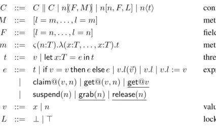
C ::= C k C | n[(F, M )] | n[n, F, L] | nhti configuration
M ::= [l = m, . . . , l = m] methods
F ::= [l = n, . . . , l = n] fields
m ::= ς(n:T ).λ(x:T, . . . , x:T ).t method definition
t ::= v | let x:T = e in t thread code
e ::= t | if v = v then e else e | v.l(~v) | v.l | v.l := v expression | claim@(v, n) | get@(v, n) | get@v
| suspend(n) | grab(n) | release(n)
v ::= x | n values
L ::= ⊥ | > lock status
Table 1. Abstract syntax
category of variables x, which we assume to be always syntactically distinguished from names n. Following a similar approach, we left undefined the syntactic category T , used to denote types: the unique assumption we make is that it includes the names c of the classes.
In general a configuration C is a collection of classes, objects, and (named) threads. The sub-entities of a configuration are composed using the parallel-construct k (which is assumed to be com-mutative and associative, as usual). The entities executing in parallel are the named threads nhti, where t is the code being executed and n the name of the thread. Threads are identified with futures, and their name is the reference under which the future result value of t will be available. A class c[(F, M )] carries a name c and defines its fields F and methods M . An object o[c, F, L], with identity o, keeps a reference to the class c it instantiates, stores the current value F of its fields, and maintains a binary lock L. The symbols >, resp. ⊥, indicate that the lock is taken, resp. free.
Besides configurations, the grammar specifies the lower level syntactic constructs, in particular, methods, expressions, and (unnamed) threads, which are basically sequences of expressions, written using the let-construct. A method ς(self :T ).λ(~x: ~T ).t provides the method body t abstracted over the ς-bound “this” parameter self , belonging to the syntactic category n, and the formal parameters ~x —the ς-binder is borrowed from the well-known object-calculus of Abadi and Cardelli [12]. Note that the methods are stored in the classes but the fields are kept in the objects. Methods lookup and field reading /modification is denoted as follows: given the method list M containing the label l, M.l yields the definition ς(self :T ).λ(~x: ~T ).t associated to l in M ; given the field list F containing the label l, F.l yields the value n associated to l in F while F [l 7→ n] returns a new field list that differs from F simply because the value associated to l becomes n.
We now list some syntactic assumptions on the user syntax, like the initial presence of one thread only, named run, or the presence in the initial configuration of the definitions for all the classes to which the objects belong.
User syntax restrictions. The most significant assumption is that, when a thread accesses a future, we impose that it corresponds to a call previously performed by the same thread. Formally, we impose that commands claim@(v, n) and get@(v, n) are such that v (denoting a future, see below) is a variable x that is bound by a corresponding let x:T = e in t, where the e expression result is obtained by: performing a method call o.l(~v) or reading a variable y satisfying, itself, the same property.
Moreover, commands claim@(x, n), get@(x, n) and suspend(n) are such that the name n (denot-ing an object on which the lock is acquired/released, see below) is the ς-bound name, denot(denot-ing the self (or “this”) object in the method where they occur. For each method definition ς(n:T ).λ(x1:T1, . . . ,
xn:Tn).t we assume that the unique variables that occur free in t are the parameter variables x1, . . . , xn.
Finally, we assume that, in user syntax, the root C of the syntactical specification, also representing the initial configuration at run-time, includes a collection of:
• any number of class definitions c[(F, M )], each one identified with a distinct class name c; • any number of instantiated objects o[c, F, L], with o being the object name, c the class name the
object belongs to (every occurrence having a different object name and referring to the name of an existing class, in such a way that there exists at least an object for each class), F being the same as the F inside the c class definition (i.e. initial value of fields is established according to field definitions) and L being ⊥ (i.e. all object locks are initially free);
• only one occurrence of a thread nhti, with n being the special thread name run (the initial thread). The body t of the initial thread, besides the constraints for standard method body definitions, must also be such that it does not include free variables x (as for a method with no parameters) and occurrences of claim, get and suspend commands (this because, for the sake of simplicity, we do not consider an initial object).
Globally, in the root C we also assume that, in methods definitions and in the initial thread run, only object names for which there exists an object instance in C may occur free. Notice that this corresponds to the restriction, we consider, of not allowing object instantiation at run-time: we thus assume identities of existing objects to be known, i.e. directly referable in the code.
Example 2.1. As an example of user defined syntax, we start with the formal presentation of (a slightly modified version of) a Creol program which has been already informally discussed in the Introduction; namely, the second one used to discuss our technique for detecting deadlocks. Consider two classes c1and c2and two initial objects o1and o2belonging to such classes, respectively. Namely,
consider the initial configuration
C0 = c1[([], [l1= m1, l3= m3])] k c2[([], [l2= m2])] k o1[c1, [], ⊥] k o2[c2, [], ⊥] k
with methods l1, l2 and l3defined as:
m1 , ς(self ).λ(). let x1= o2.l2(1) in
let x2= o2.l2(5) in
get@(x2, self ) ; (claim@(x1, self ); 0)
m2 , ς(self ).λ(x). ( if x = 1 then 0 else (let x3= o1.l3() in claim@(x3, self )) ) ; 0
m3 , ς(self ).λ(). 0
Notice that, for simplicity, we have omitted type declarations and, if compared with the corresponding example in the Introduction, we avoid some useless parameter passings as well as some arithmetic operations.
Creol programs behaviour. Methods are called asynchronously, i.e., executing o.l(~v) creates a new thread to execute the method body with the formal parameters appropriately replaced by the actual ones; the corresponding thread identity at the same time plays the role of a future reference, used by the caller to obtain, upon need, the eventual result of the method. The further expressions claim, get, suspend, grab, and release deal with communication and synchronization. As mentioned, objects come equipped with binary locks which assures mutual exclusion. The operations for lock acquisition and release (grab and release) are run-time syntax and inserted before and at the end of each method body code when invoking a method. Besides that, lock-handling is involved also when futures are claimed, using claim or get. The get@(x, o) operation is easier: it blocks if the result of the future n in x is not (yet) available, i.e., if, at run-time, the thread n is not of the form of nhn0i, with n0being
the returned value. The claim@(x, o) is a more “cooperative” version of get@(x, o): if the value is not yet available, it releases the lock of the object o (it executes in) to try again later, meanwhile giving other threads the chance to execute in that object.
As usual we use sequential composition e; t as syntactic sugar for let x:T = e in t, when x does not occur free in t. We refer to [10] for further details on the language constructs, a type system for the language and a comparison with the multi-threading model of Java.
2.2. Operational Semantics
Axioms and rules of the operational semantics are shown in Table 2, where reduction steps are de-noted by labeled transitions dede-noted with−→. The label λ, ranging over the set of possible labelsλ {τ, n, [n1, n2, o.l]}, is used to carry information that will be useful in Definitions A.1, A.2, and A.3.
More specifically, the labels have the following meaning: label n means that the return value of the thread n is accessed, [n1, n2, o.l] stands for a method call executed by thread n1on method l of object
o with creation of a new thread n2, while τ does not carry specific information (hence it is usually
omitted).
As usual in reduction semantics, axioms assume to have the components involved in the step in predefined positions w.r.t. the k composition operator: commutativity and associativity of such operator are used to readjust the order of the components in such a way the axiom can be applied. A
nhlet x:T = n0in ti → nht[n0/x]i RED
nhlet x:T = (let x0:T0 = e0in t0) in ti → nhlet x0:T0= e0in(let x:T = t0in t)i LET
nhlet x:T = (if n = n then e1else e2) in ti → nhlet x:T = e1in ti COND1
nhlet x:T = (if n1= n2then e1else e2) in ti → nhlet x:T = e2in ti with n16= n2 COND2
o[c, F, L] k nhlet x:T = o.l in ti → o[c, F, L] k nhlet x:T = n0in ti with n0= F.l FLOOKUP
o[c, F, L] k nhlet x:T = (o.l := n0) in ti →
o[c, F0, L] k nhlet x:T = n0in ti with F
0= F [l 7→ n0] FU PDATE
c[(F0, M )] k o[c, F, L] k n1hlet x:T = o.l(~v) in t1i
[n1,n2,o.l]
−−−−−−→ c[(F0, M )] k o[c, F, L] k n1hlet x:T = n2in t1i k
n2hlet y:T2= (grab(o); t2) in release(o); yi
with n2fresh
and t2= M.l(o)(~v)
FUT
n1hni k n2hlet x:T = claim@(n1, o) in ti n1
−→ n1hni k n2hlet x:T = n in ti CLAIM1
n1ht1i k n2hlet x:T = claim@(n1, o) in t2i n1
−→
n1ht1i k n2hlet x:T = (release(o); get@n1) in grab(o); t2i
with 6 ∃n : t1 = n CLAIM2
n1hni k n2hlet x:T = get@(n1, o) in ti n1
−→ n1hni k n2hlet x:T = n in ti GET1
n1hni k n2hlet x:T = get@n1in ti n1
−→ n1hni k n2hlet x:T = n in ti GET2
nhsuspend(o); ti → nhrelease(o); (grab(o); t)i SUSPEND
o[c, F, ⊥] k nhgrab(o); ti → o[c, F, >] k nhti GRAB
o[c, F, >] k nhrelease(o); ti → o[c, F, ⊥] k nhti RELEASE
C1 −→ Cλ 10
CONTEXT
C1 k C2 −→ Cλ 10 k C2
contextual rule is then considered to lift the computation step to a richer configuration that contains also other components besides those directly involved in the reduction.
An execution is a sequence of configurations, C0, . . . , Cnsuch that Ci+1is obtained from Ciby
applying a reduction step−→. We denote executions by Cλ 0 −→ . . . −→ Cnomitting, for simplicity, the
transition labels.
Invoking a method (cf. rule FUT) creates a new future reference and a corresponding thread is
added to the configuration. In the configuration after the reduction step, the notation M.l(o)(~v) stands for t[o/s][~v/~x], when M.l is ς(s:T ).λ(~x: ~T ).t. Here and in the following, we use the t[v/x] notation to denote the result of syntactically replacing x by v in the thread code t. As usual, only free variables are replaced: in this context the variable binding operator is the let statement. The notation above is extended to vector replacement [~v/~x], standing for replacement of each variable in ~x by the value in ~v that is placed in the same vector position. Similarly, we use t[n0/n] to denote syntactical replacement of a name n by another name n0 (notice that in thread code t there are no binders for names). Upon termination, the result is available via the claim- and the get-syntax (cf. the CLAIM- and GET-rules), but not before the lock of the object is given back again using release(o). If the thread is not yet terminated, in the case of claim statement, the requesting thread suspends itself, thereby giving up the lock. The rule SUSPEND releases the lock to allow for interleaving. To continue, the thread has to re-acquire the lock. Other reduction rules are straightforward.
Example 2.2. To show how the operational semantics rules can be applied to a configuration, we now present a couple of reduction steps starting from the initial configuration C0 defined in the Example
2.1. By applying rules FUTand CONTEXTwe have C0
[run,n1,o1.l1] −−−−−−−−→ C1with C1 = c1[([], [l1= m1, l3= m3])] k c2[([], [l2= m2])] k o1[c1, [], ⊥] k o2[c2, [], ⊥] k runh let x = n1in 0 i k n1h let z = grab(o1); let x1= o2.l2(1) in
let x2= o2.l2(5) in ( get@(x2, o1); (claim@(x1, o1); 0) )
in (release(o1); z) i
By applying rules GRABand CONTEXTwe have C1 → C2 with
C2 = c1[([], [l1= m1, l3= m3])] k c2[([], [l2= m2])] k o1[c1, [], >] k o2[c2, [], ⊥] k
runh let x = n1in 0 i k
n1h let z =
let x1= o2.l2(1) in
let x2= o2.l2(5) in ( get@(x2, o1); (claim@(x1, o1); 0) )
in (release(o1); z) i
In the continuation of the above computation we have that the method l2 of o2 is invoked twice with
second one it invokes l3on o1. Namely, the following configuration is reached (assuming n2, n3and
n4be the fresh thread names used to identify the two invocations of method l2on o2and method l3on
o1, respectively):
C = c1[([], [l1= m1, l3= m3])] k c2[([], [l2= m2])] k o1[c1, [], >] k o2[c2, [], >] k
runh let x = n1in 0 i k
n1h let z = get@(n3, o1); (claim@(n2, o1); 0) in (release(o1); z) i k
n2h0i k
n3h let z = (claim@(n4, o2); 0) in (release(o2); z) i k
n4h let z = (grab(o1); 0) in (release(o1); z) i
This, however, will cause object o1 to block indefinitely; in fact, thread n4 will never acquire the
o1 lock because n1remains blocked while holding such lock. This happens because n1waits for n3,
that waits for n4, which is blocked by n1.
3.
Deadlock
As we already explained in the Introduction, we give two different notions of deadlock in Creol. The first one, we call classical deadlock, follows [4]. In this case not only threads are blocked but also the objects hosting them, as it happens in the above Example 2.2. The second notion, we call extended deadlock, resembles the definition of deadlock by Holt [8]. In this case, instead of looking at blocked objects we look at blocked threads. A blocked thread does not necessarily block the object hosting it. Before formally defining these two notions of deadlock, we consider again the first example we presented in the Introduction: the example of classical deadlock and, by modifying one method, of extended deadlock. We now present (a slightly modified version of) the Creol program for such an example and we give a formal argument for it to originate a classical/extended deadlock.
Example 3.1. Consider an initial configuration including two objects o1and o2both of class C
defin-ing methods l1, l2and l3. Concerning methods, their definitions m1, m2and m3, respectively, are the
following ones (also in this case, for simplicity type declarations are omitted): m1 , ς(self ).λ(x). let x1= o2.l2() in
let x2 = (if x = 1 then get@(x1, self ) else 0) in x2
m2 , ς(self ).λ(). let y1= o1.l3() in (let y2= get@(y1, self ) in y2)
m3 , ς(self ).λ().1
Calling method l1 on object o1 with parameter value 1, that is considering the run thread in the
initial configuration to be, e.g.,
runhlet x = o1.l1(1) in 0i
Formally, starting from the initial configuration, and assuming n1, n2and n3to be the fresh thread
names created by the operational semantics (rule FUT) when executing method calls o1.l1(1), o2.l2()
and o1.l3(), respectively, the program reaches a configuration whose threads in execution are:
• runh0i
• n1hlet x2 = get@(n2, o1) in ( let z = x2in (release(o1); z) )i
• n2hlet y2= get@(n3, o2) in ( let z = y2in (release(o2); z) )i
• n3hlet z0 = grab(o1) in ( let z = 1 in (release(o1); z) )i
Since in such a configuration the locks of the objects o1 and o2 are both taken (this can also be seen
from the fact that the first statement of threads n1and n2is get@(n2, o1) and get@(n3, o2), thus they
own the o1and o2object lock, respectively) the above threads can no longer proceed in the execution.
As we will see from the following Definition 3.4, this configuration is a classical deadlock. Consider now the case in which method l2has, instead, the following definition m2:
m2 , ς(self ).λ(). let y1= o1.l3() in (let y2= claim@(y1, self ) in y2)
In this case, assuming again thread names created during execution to be n1, n2 and n3, the
program reaches a configuration where threads run, n1and n3are as above, while n2is:
• n2hlet y2= get@n3in ( grab(o2); let z = y2in (release(o2); z) )i
As we will see from the following definitions, this configuration is not a classical deadlock (Definition 3.4), in that object o2is not actually blocked because thread n2does not own the lock (this can be seen
from the fact that the first statement of thread n2 is get@n3). On the contrary, we will see that this
reached configuration is instead an extended deadlock (Definition 3.5).
The example above of extended deadlock will be our running example throughout the paper.
To facilitate the definition of deadlock we introduce the notions of waiting and blocking threads. The notion of a waiting thread links a thread to another one or to an object. In the first case, it is waiting to read a future that the other thread has to calculate. In the second case, the thread is waiting to obtain the lock of the object.
Definition 3.2. (Waiting Thread) A thread n1hti is waiting for:
1. “n2” iff t is of the form let x:T = get@(n2, o) in t0 or let x:T = get@n2in t0;
2. “o” iff t is of the form let x:T = grab(o) in t0
The notion of a blocking thread links a thread that is waiting for a future while holding the lock of the object.
Definition 3.3. (Blocking Thread)
Note that a thread needs to hold the object lock and execute a blocking statement, i.e. get-statement, to block that object. Furthermore note that the threads can at most acquire one lock, i.e. the lock of its hosting object.
Our notion of a classical deadlock follows the definition of deadlock by Coffman Jr. et al.[4]. The source of interest is the exclusive access to an object represented by the object lock. In opposite to other multithreaded settings, e.g. like in Java, where a thread can collect a number of these exclusive rights, a thread in our active object setting can at most acquire the lock of the object hosting it. But by calling a method on another object and requesting the result of that call it requires access to that object indirectly. To be more precise, a thread can derive the information that the thread created to handle its call had access to the lock of the called object, by checking the availability of the result inside the corresponding future.
Definition 3.4. (Classical Deadlock)
A configuration C is a classical deadlock iff there exists a set of objects O such that the following holds. For all o ∈ O, o is blocked by a thread n1 that is waiting for a thread n2 such that: for some
object o0∈ O, either n2blocks o0or n2is waiting for o0.
Note that the definition of “waiting for” plays a crucial role here, because while a thread is waiting, it cannot finish its computation. Being blocked by threads, the objects in O cannot execute other threads. But also the threads blocking the objects cannot proceed because they are indeed waiting for one of such non-executing threads. This generates a classical deadlock situation. Note that a blocking thread does not necessarily directly wait for another blocking thread but can also wait for a thread which is simply waiting to have access to its object in O.
The second notion resembles the definition of deadlock by Holt [8]. Instead of looking at blocked objects we look at blocked threads. A thread can be blocked due to the execution of either a get– statement or a claim–statement. In the first case the object is blocked by the thread, in the second case only the thread is blocked. Threads that are blocked on a claim–statement are not part of a deadlock according to the first definition since they are not holding any resource. Yet they can be part of a circular dependency that prevents them from making any progress.
Definition 3.5. (Extended Deadlock)
A configuration C is an extended deadlock iff there exists a set of threads N such that, for all n1∈ N ,
n1 is waiting for n2∈ N , or waiting for some object o that is blocked by n2 ∈ N .
We require the set of threads to be finite in order to guarantee circularity. This notion of deadlock is more general than the classical one.
Proposition 3.6. Every classical deadlock is an extended deadlock.
Proof: Let O be the set of objects involved in a classical deadlock. We denote by B(O) the set of threads blocking an object in O and by W (B(O)) the set of threads the threads in B(O) are waiting for. Consider N = B(O) ∪ W (B(O)): it is a finite set of threads. It remains to show that for all n1 ∈ N , n1 is waiting for n2∈ N , or waiting for o which is blocked by n2∈ N .
By definition of classical deadlock and W (B(O)) each thread n1 ∈ B(O) is waiting for a thread
n2 ∈ B(O) ∪ W (B(O)) = N . Thus each thread n1 ∈ B(O) is waiting for a thread n2 ∈ N .
We now consider the remaining threads in N , i.e. the threads n1 ∈ W (B(O)). By definition of
classical deadlock and W (B(O)) such threads are either in B(O) or waiting for an object o ∈ O. In the former case n1 ∈ B(O) and the above reasoning applies. In the latter, by definition of classical
deadlock and B(O), this object o is blocked by a thread n2 ∈ B(O) ⊆ N , i.e. n1 is waiting for o
which is blocked by a thread n2 ∈ N .
4.
Translation into Petri nets
We translate Creol programs into Petri nets in such a way that extended deadlocks in a Creol program can be detected by analyzing the reachability of a given class of markings (that we will call extended deadlock markings) in the corresponding Petri net.
4.1. Petri nets preliminaries
We first recall the definition of Petri nets. We adopt a simplified definition without explicit mention of the flow relations, which are replaced by the assumption that each transition t comes equipped with a preset•t and a postset t•, respectively indicating the places from which tokens are consumed, and where tokens are introduced, by the transition t.
Definition 4.1. (Petri nets)
A Petri net is a tuple hP, T, m0i such that P is a finite set of places, T is a finite set of transitions,
and m0is the initial marking, i.e. a function from P to N0 that defines the initial number of tokens in
each place of the net. A transition t ∈ T is characterised by a function•t (preset) from P to N0, and
a function t• (postset) from P to N0: the preset indicates the tokens that must be consumed to fire a
transition, the postset indicates the tokens that are produced as effect of such firing.
Concerning Petri net execution, this is represented as a sequence of configurations that are rep-resented by markings m. Formally, transition t is enabled at marking m iff •t(p) ≤ m(p) for each p ∈ P . Enabled transitions can fire. Firing t at m leads to a new marking m0 defined as m0(p) = m(p) −•t(p) + t•(p), for every p ∈ P . A marking m is reachable in a Petri net hP, T, m0i
if m = m0 or if, starting from m0, it is possible to produce m by firing finitely many (enabled)
transitions in T .
Despite Petri nets are infinite state systems because the number of tokens that can be generated could be unbounded, many interesting properties are decidable, for instance marking reachability [13] (i.e. a given marking m is reachable in a given Petri net) and coverability [14] (i.e. there exists a marking greater2 than a given marking m that is reachable). We will use a more expressive form of reachability that was studied in [15]: target marking reachability.
2A marking m0
Definition 4.2. (Target marking reachability)
Let P = hP, T, m0i be a Petri net. A target marking denotation is a pair of functions (inf, sup) ∈
(P → N0) × (P → (N0 ∪ ∞)) (with N0 denoting the set of non-negative integers) such that for all
p ∈ P we have inf (p) ≤ sup(p) (assuming n ≤ ∞ for all n ∈ N0). We say that a marking m satisfies
a target marking denotation (inf, sup) if, for all p ∈ P , we have inf (p) ≤ m(p) ≤ sup(p). Target marking reachability is the problem of checking, given a Petri net P and a target marking denotation (inf, sup), whether there exists a marking satisfying (inf, sup) that is reachable in P.
In [15] it is shown that target marking reachability is decidable; intuitively, this follows from the fact that it can be reduced to a combination of reachability and coverability that, as recalled above, are both decidable for Petri nets.
4.2. Informal introduction to the Petri net encoding of Creol
In Creol a fresh unique thread name is created for each method invocation, implying that unboundedly many distinct futures can be created during the computation of a Creol program. As Petri nets are finite, it is not possible to represent such unbounded distinct names faithfully. For this reason, we perform an abstraction: thread names are abstractly identified by a tuple of caller object o, calling method l, callee object o0, and called method l0. We denote this tuple with [email protected]. It is interesting to observe that even if we will use in the Petri net finitely many abstract thread names, we still allow for an unbounded number of method invocations. In fact, active threads will be represented with tokens, and there is no a-priori limit to the number of tokens that can be produced within a Petri net.
In the Petri net, we will have two kinds of places: those representing a method code to be executed by a given object, and those representing object locks. The restriction to a version of Creol without object creation allows us to keep the Petri net finite, otherwise we will have to consider unboundedly many places for the object locks. Moreover, in the places representing the method code to be executed, we abstract away from the data that could influence such method (like, e.g., the object fields or the actual value of the passed parameters) otherwise we would need infinitely many places.
As discussed above, the threads and the corresponding futures are abstractly represented in the Petri net by using the finite set of tuples [email protected]. Due to this abstraction the Petri net semantics could have the following token swap problem. If there are two invocations of the same method l0 on the object o0, performed by the method l of the object o, these two invocations will be indistinguishable in the Petri net as both will be abstractly identified with [email protected]. More precisely, both futures will be placed in the same place (hence generating token swap).
As an example of token swap, consider the Creol program in the Example 2.2. In the reported configuration C we have the threads n2 and n3 that correspond to the execution of the method l2
on object o2, invoked by the method l1 on object o1. This means that the abstract name for both n2
and n3is [email protected]. Having the same name, the thread n1 which is concretely waiting for n3, will
abstractly wait for any possible return value on [email protected]. A return value on this abstract name
is available, namely the return value of the concrete thread n2, hence thread n1 will wrongly read
such value in the abstract semantics. Token swap identifies this precise phenomenon occurring in the abstract semantics. In this particular case, token swap will avoid the deadlock because thread n1
entire program to complete without any deadlock.
We now discuss two techniques that we will adopt to limit the effect of the token swap problem: limitation of the propagationand abstract name tagging.
To avoid the propagation of the token swap problem, in the Petri net, as soon as a caller accesses to a return value in a future, such value is consumed. In this way, we assign the future to a concrete caller and consuming the future prevents it from being claimed by two different threads. To apply this technique in a sound way we have to transform the program. Removing the future upon first claim implies that it is not available for subsequent accesses. Nevertheless, subsequent accesses do not provide any new information with respect to deadlock detection because in the Creol semantics once a future has been accessed it remains available for all subsequent accesses that immediately successfully pass. In the Petri net semantics we simply model this by transforming the program by removing the accesses to a future that has been already accessed.
Internal choice is an obstacle with respect to this approach. In a sequence of internal choices the kind of a claim (first or subsequent) depends on the choices taken so far and can vary depending on them. To overcome this problem we also linearize programs by moving all internal choices up front.
But this approach only allows to avoid the token swap for sequential identical abstract thread names. In the case of concurrent identical abstract names this is not enough. To address this problem each method invocation, generating a fresh thread name in the operational semantics, can be nonde-terministically tagged or not. When a thread tags one of its call, all the subsequent calls will be not tagged. A tagged call to method l of object o will be denoted with o.l?.
The intuition behind the tagging of method calls is that the Petri net semantics will surely include a computation that tags only the calls that will be directly involved in the deadlock, in such a way that it will be not possible to have the token swap problem at least on such calls. More precisely, we will have the guarantee that every computation in Creol that leads to a deadlock will be reproduced in the abstract Petri net semantics by a computation that tags only the calls generating threads on which the deadlocking get statements are executed. For instance, the computation leading to a deadlock discussed at the end of the Example 2.2, will be reproduced by the Petri net execution in which the first call is not tagged while the second one is. In this execution, the deadlocking get will be executed on a place labeled with [email protected]? that is not swapped with the place filled by the first call that will
be labeled with [email protected].
4.3. Generation of Abstract Statement Traces
We now present some preliminary formal machinery necessary to define our Petri net encoding. First of all, we need to introduce an abstract representation for method definitions. As previously discussed, we linearize the code to remove intermediary nondeterminism; more precisely, we will define a way to extract from a Creol method definition a set of possible traces composed of abstract statements, each of these sequence represents a possible execution.
Definition 4.3. (Statement Trace)
An abstract statement ast is a statement of the following form: ast ::= let o.l | get@(o.l, o) | [email protected]
| let o.l? | get@(o.l?, o) | [email protected]? | release(o) | grab(o)
An (abstract) trace is a “;” separated sequence of abstract statements. On statement traces we consider the following algebra: “;” denotes sequence concatenation and ε denotes the empty sequence, which is the identity element of “;” (i.e. given a sequence w, we assume w; ε and ε; w to yield w). Moreover we say that a trace w0is a suffix of trace w whenever there exists w00such that w = w00; w0.
The abstract statements are of four types: (i) creation of abstract future names —tagged (i.e. o.l?) or non tagged (i.e. o.l)—, (ii) access to an abstract future by means of a get statement (there are two kinds of get, those that block the object o of the executing thread, and those that do not block the object), and (iii) the request to acquire or release the object lock.
Notice that the Creol statements if then else, suspend and claim are no longer present among the abstract statements. The conditional statements are removed as effect of code linearization while, following the Creol operational semantics, the suspend statements are abstractly represented as se-quences of release–grab and, similarly, claim commands become sese-quences of release–get–grab.
It is worth to notice that this last transformation does not faithfully correspond to the operational semantics of claim. In fact, the claim statement follows a conditional release policy: if the claimed future is not yet available the lock is released, on the contrary, if the claimed future is available the thread continues without releasing the lock. Differently, in the abstract interpretation of claim the lock is always released. This discrepancy is not observable on those claim that are preceeded by operations accessing the same future; indeed, as explained above, we completely abstract away from such claim. On the contrary, if a claim is the first command that accesses a future, this difference becomes observable. Nevertheless, as we will discuss in the following, this is not problematic for two main reasons. The first one is that the concrete computation that accesses the future without releasing the lock can be any way reproduced in the abstract semantics as a sequence of release–grab and access to the future. The second reason is that the additional computations that are present in the abstract semantics due to the lock release will be non problematic for our analysis: as we will show, the abstract semantics is an over-approximation of the possible concrete computations.
Abstract statement traces are obtained by applying to method definitions (and the initial thread) a sequence of syntactical transformations informally defined as follows:
Step one s1. It takes Creol code t and applies data abstraction (and replacement of variables that are
not defined by means of method calls) to it, obtaining abstracted code in the form of a tree. Step two s2. It turns abstracted code (a tree) into a set of sequences, representing possible executions
of the method (i.e. turning all intermediate choices into a single initial choice).
Step three s3. For each sequence it removes the redundant claims/gets of a future, i.e. the claims/gets
operational semantics, each claim statement by a sequence of release, get and grab statements. Similarly it also replaces each suspend statement by a release followed by a grab.
Step four s4. For each sequence it returns a set of sequences (which are then put together to form an
overall set of sequences): it yields all possible sequences obtained by tagging, inside it, at most one of its get. Notice that the sequence itself (without any tag) is also included among returned sequences. As we already explained, tagging is used to explicitly tag the case we are getting a future of a method call (thread) that is involved in a deadlock.
Step five s5. For each sequence it applies future abstraction, replacing future parameter x of get
oc-currences with the pair o.l, i.e. called object “o” and called method “l”, retrieved from the method call performed inside the definition of variable x.
Concerning sequences (used in the output of the s2 step and in the input and output of all
subse-quent steps) we will use the same notation we introduced for abstract statement traces of Definition 4.3. In addition we will consider concatenation “;” of pair of sequences to be extended to sets of sequences, with the usual definition: w; W = {w; w0 | w0 ∈ W } and W ; w = {w0; w | w0 ∈ W }, with w a sequence and W a set of sequences. At every step will consider sequences over a different set of statements: such a set will be detailed in the definition of the functions, presented below.
Formally the overall transformation, takes Creol code t, with t being such that 1. runhti occurs in the initial configuration or
2. t = ˆt[o/self ] for some object o, method l and class c, with c[(F, M )] and o[c, F, ⊥] occurring in the initial configuration and M.l = ς(self :T ).λ(~x: ~T ).ˆt
and yields a set of abstract statement traces of Definition 4.3. Such a transformation is called ST (Statement Traces) and is defined as the composition of all above functions:
ST , s5◦ s4◦ s3◦ s2◦ s1
In the following we will formally define the s1, s2, s3, s4and s5functions.
For all trees/sequences considered in the input and output of the various steps (apart from those of Definition 4.3 obtained by applying the final step s5 where future variables x do not occur) the
following property holds: each claim/get statement uses a future parameter x that is bound by a let declaration of variable x occurring previously in the tree/sequence. This is a consequence of the syntactical restrictions we considered over initial configurations (and of the fact that each step preserves this property).
Moreover, we assume, without loss of generality, that in the initial Creol code t (to which the 5 chained steps of ST are applied) we use a different variable name in each variable let declaration occurring inside it: if this is not the case we can just change variable names in the code. As long as this is guaranteed, ST(t) yields the same set of abstract statement traces, no matter the specific name chosen for the variables.
Finally it is worth observing that the transformation functions (in particular the s1 function) are
given a class c occurring in the initial configuration, we will use O(c) to denote the set of all objects o of class c occurring in such a configuration. Notice that, due to the syntactical restrictions that we considered, O(c) cannot be empty.
4.3.1. Step one: s1 (Data abstraction).
This step receives, as input, Creol code t, obtained from the initial run thread or the body of a method, as described above. We remove most data from t, keeping only the objects names “o” (which are all free, due to the syntactical restrictions that we considered and since, in the case of methods bodies, we replaced self by the object name that is executing the method) and the future variables “x”. Moreover, we replace all variables that are not defined by means of method calls, removing the corresponding let declarations. Thus the only let declarations that are left are future variables defined by means of method calls, which are abstracted by removing parameter data and are simply denoted by let x:T = o.l. This is a first step in obtaining the abstract statements for method invocations of Definition 4.3. Conditional (on data) branching is replaced by non-deterministic internal choice. Concerning method invocations on object variables x (e.g. being x a method parameter or a let declared variable that is initialized with the object contained inside a field/returned by a method), we replace the concrete invocation by a non-deterministic choice amongst all possible invocations, i.e. given the class type T of x, all objects in the initial configuration belonging to that class. In the definition we make use of the following auxiliary functions. Given a variable x occurring in the Creol code t given as input to s1,
T (x) denotes the type T of the variable (taken from its declaration, i.e. a let declaration or a method formal parameter declaration).
Transformation s1 outputs abstract code, i.e. a tree whose branches are labeled by statements,
ranged over by st, and alternative branches represent abstraction of if-then-else statements. Abstract code, ranged over by ac, belongs to the syntax
ac ::= ε | st; ac | ac + ac
st ::= let x = o.l | claim@(x, o) | get@(x, o) | suspend(o)
where we use “+” to denote alternative abstract codes,“;” to separate a branch from the abstract code (subtree) it leads to, and ε to denote empty abstract code.
s1(v) , ε
s1(let x:T = v in t) , s1(t[v/x])
s1(let x:T = (let x0:T0 = e0in t0) in t) , s1(let x0:T0= e0in(let x:T = t0in t))
s1(let x:T = claim@(x0, o) in t) , claim@(x0, o); s1(t)
s1(let x:T = get@(x0, o) in t) , get@(x0, o); s1(t)
s1(let x:T = suspend(o) in t) , suspend(o); s1(t)
s1(let x:T = (v.l := v0) in t) , s1(t[v0/x])
s1(let x:T = v.l in t) , s1(t)
s1(let x:T = (if v1= v2then e1else e2) in t) , s1(let x:T = e1in t)+s1(let x:T = e2in t)
s1(let x:T = o.l(~v) in t) , let x = o.l; s1(t)
s1(let x:T = x0.l(~v) in t) , Σo∈O(T (x0)) let x = o.l; s1(t[o/x0])
Notice that the sum in the last defining equation has at least one argument (since class T (x0), due to the syntactical restrictions, must occur in the initial configuration, we have that, as observed above, O(T (x0)) cannot be empty). In the case such a sum has one argument only, then it is assumed to just yield such an argument; otherwise, in the case of n ≥ 1 arguments ac1, . . . , acn, it yields
ac1+ · · · + acn, where the way in which the binary + is associated is not significant.
Example 4.4. Consider the extended deadlock example presented in Example 3.1 that we use as a running example.
Let t1, t2 and t3 be the Creol code of methods l1, l2 and l3, respectively, of class C. That is, for
each i ∈ {1, 2, 3}, ti is such that mi = ς(self :Ti).λ( ~xi: ~Ti).ti. Observe that ~x1just contains variable
x, while ~x2and ~x3are empty.
We have (for simplicity, since we do not have method calls on variables and function T () is not used, type declarations are omitted):
• t1 , let x1 = o2.l2() in (let x2= (if x = 1 then get@(x1, self ) else 0) in x2)
• t2 , let y1 = o1.l3() in (let y2 = claim@(y1, self ) in y2)
• t3 , 1
Moreover let t be the Creol code of the run thread, i.e.: • t , let x = o1.l1(1) in 0
We now consider the Creol code of methods l1, l2and l3 when executed by some object o of class
C, i.e. t1[o/self ], t2[o/self ] and t3[o/self ], respectively.
• s1(t1[o/self ]) = let x1= o2.l2; ( (get@(x1, o); ε) + ε )
• s1(t2[o/self ]) = let y1= o1.l3; (claim@(y1, o); ε)
• s1(t3[o/self ]) = ε
• s1(t) = let x = o1.l1; ε
Notice that all variables were removed except for future variables x1, y1and x.
4.3.2. Step two: s2(Unification of choice).
This step receives, as input, abstracted code ac, i.e. a tree whose branches are labeled over st state-ments. Since all choices are internal we can anticipate them and perform a single global choice at the beginning, which selects among possible execution traces.
This step outputs a set of sequences, representing execution traces, over st statements. Notice that such sequences are finite because method code, itself, does not include looping constructs (looping is expressed/encoded by recursion). The idea in turning the ac tree into a set of sequences is that, for each of them it is clear whether or not the result of a method call is read later by a claim/get or not.
We formalize this step via a function s2, defined as follows.
s2(ε) , {ε} s2(ac1+ ac2) , s2(ac1) ∪ s2(ac2)
s2(st; ac) , st; s2(ac)
Example 4.5. By applying step 2 to our running example, we get: • s1,2(t1[o/self ]) = { let x1= o2.l2; get@(x1, o) , let x1= o2.l2 }
• s1,2(t2[o/self ]) = { let y1= o1.l3; claim@(y1, o) }
• s1,2(t3[o/self ]) = { ε }
• s1,2(t) = { let x = o1.l1 }
where, given Creol code t0, we use s1,2(t0) to stand for s2(s1(t0)). In general in the following we will
use, for the sake of conciseness, s1,k(t0), with k ≤ 5, to stand for sk(. . . (s1(t0)) . . . ).
4.3.3. Step three: s3(Transformation of communication).
This step receives, as input, a set of sequences over st statements. For each sequence it removes the redundant claims/gets of a future, i.e. the claims/gets that, for a given future, occur in the code after the first one. Since we are abstracting from data (including data returned by methods) we can just remove claims/gets occurring after the first one. This allows us to represent, in Petri nets, reading of futures as token consumption from the place representing the future. This because, by guaranteeing
that future reading can occur at most once, the Petri net will not block in trying to consume a token that has already been consumed by a previous reading of the same future.
In addition this step replaces, as done by Creol operational semantics, each claim statement by a sequence of release, get and grab statements. This is done in order to move from static syntax to run-time syntax (which actually represents, at a lower level, the code behavior) and to do a further step in the direction of obtaining abstract statements of Definition 4.3. Similarly it also replaces each suspend statement by a release followed by a grab. Transformation s3 outputs a set of strings over
run-timestatements rst defined by the grammar
rst ::= let x = o.l | get@(x, o) | get@x | release(o) | grab(o)
We formalize this step via a function sF3, with F being a set of future variables x, that transforms a single st sequence into a rst sequence. The sF3 function is defined inductively and, while F is assumed to be initially empty (F = ∅), during the induction it contains the set of variables whose futures have been already consumed. Function sF3 is defined as follows.
sF
3(let x = o.l; t) , let x = o.l; sF3(t)
sF3(claim@(x, o); t) , (
release(o); get@x; grab(o); sF ∪{x}3 (t) if x /∈ F
sF3(t) if x ∈ F sF3(get@(x, o); t) , ( get@(x, o); sF ∪{x}3 (t) if x /∈ F sF 3(t) if x ∈ F
sF3(suspend(o); t) , release(o); grab(o); sF3(t)
sF3(ε) , ε
The s3 transformation is obtained by lifting sF3 to work over sets of strings, so that it can be
chained with the s2 transformation.
sF
3(W ) , {sF3(t) | t ∈ W }
The s3transformation is therefore defined as s∅3(W ), where W is the set of st sequences outputed
by s2. For the sake of simplicity, we will just write s3to stand for s∅3.
Example 4.6. By applying step 3 to our running example, we get: • s1,3(t1[o/self ]) = { let x1= o2.l2; get@(x1, o) , let x1= o2.l2 }
• s1,3(t2[o/self ]) = { let y1= o1.l3; release(o); get@y1; grab(o) }
• s1,3(t3[o/self ]) = { ε }
• s1,3(t) = { let x = o1.l1 }
The claim statement was replaced in the second set. Notice that, this is the only change in the traces because all of them only have at most one get/claim statement.
4.3.4. Step four: s4 (Adding Tags).
This step receives, as input, a set of sequences over rst statements. For each sequence it produces a set of sequences: all possible sequences obtained by tagging, inside it, at most one of its get with the “?” symbol. This means that the sequence itself (without any tag) is also included among the produced sequences. The idea is that, if the input code (an execution sequence) is involved in a deadlock by means of one of its get, i.e. it is blocked on such a get, then that it is obviously not possible that, in the context of the same deadlock, it is blocked also on other get. Of course it can be that it is not involved at all in the deadlock, i.e. it has no tag. More formally, given an extended deadlock reached by a Creol program, we have that each thread n belonging to the set N of Definition 3.5 may block on a grab or on a get of a future/thread n0. In the latter case, in order to detect such a deadlock in the Petri net, we consider a tagged abstract identifier in the form [email protected]? for the thread n0. Thus we have to consider a possible sequence for the code of n where get is correspondingly tagged. Of course, whenever we tag a get, we have also to tag with the “?” symbol the let statement binding it, which performs the o.l method call (generating the thread with the [email protected]? abstract identifier).
Transformation s4 outputs a set of strings over a tagged run-time statements mst defined by the
grammar
mst ::= rst| let x = o.l? | get(x?, o) | get@x?
We formalize this step via a function s4, which transforms a single rst sequence into a set of mst
sequences, defined as follows.
s4(t) , {t} ∪ {t1; let x = o0.l?; t2; get(x?, o); t3 | t = t1; let x = o0.l; t2; get(x, o); t3}
∪ {t1; let x = o0.l?; t2; get@x?; t3 | t = t1; let x = o0.l; t2; get@x; t3}
This definition is based on the fact (discussed before) that, in traces produced by previous steps: for each get statement using a future parameter x there is one and only one let declaration of x occurring previously in the sequence.
The s4 transformation is obtained by lifting function s4 to work over sets of strings, so that it can
be chained with the s3transformation.
s4(W ) , ∪t∈Ws4(t)
where W is the set of rst sequences outputed by s3.
Notice that the sets of sequences produced, for each input sequence, by the s4 function, are put
together to form an overall set of sequences, which is the output of the s4transformation.
Example 4.7. By applying step 4 to our running example, we get: • s1,4(t1[o/self ]) =
• s1,4(t2[o/self ]) =
{ let y1= o1.l3; release(o); get@y1; grab(o) ,
let y1= o1.l3?; release(o); get@y1?; grab(o) }
• s1,4(t3[o/self ]) = { ε }
• s1,4(t) = { let x = o1.l1 }
4.3.5. Step five: s5(Future abstraction).
This step receives, as input, a set of sequences over mst statements. In this last step we apply future abstraction, thus removing future variables. Up until now, they were preserved because they were necessary to define the function s4. More precisely, we replace future parameter x of get occurrences
with the pair o.l, i.e. called object “o” and called method “l”, retrieved from the method call per-formed inside the definition of variable x. Transformation s5 outputs a set of statement traces (see
Definition 4.3), i.e. sequences over abstract statements ast.
We formalize this step via a function s5that transforms a single mst sequence into an ast sequence.
Function s5 is defined as follows.
s5(let x = o.l∗; t) , let o.l∗; s5(t)[o.l/x]
s5(mst; t) , mst; s5(t) 6 ∃x, o, l : mst ∈ {let x = o.l, let x = o.l?}
where “∗” is a meta-variable that can be either the empty string or “?” (used to denote that “let x = o.l” can be tagged or not) and “t[o.l/x]” is the result of replacing “x” by “o.l” in “t”.
The s5transformation is obtained by lifting function s5 to work over sets of sequences, so that it
can be chained with the s4transformation.
s5(W ) , {s5(t) | t ∈ W }
Example 4.8. By applying step 5 to our running example, we get: • s1,5(t1[o/self ]) = ST(t1[o/self ]) =
{ let o2.l2; get@(o2.l2, o) , let o2.l2?; get@(o2.l2?, o) , let o2.l2 }
• s1,5(t2[o/self ]) = ST(t2[o/self ]) =
{ let o1.l3; release(o); [email protected]; grab(o) ,
let o1.l3?; release(o); [email protected]?; grab(o) }
• s1,5(t3[o/self ]) = ST(t3[o/self ]) = { ε }
o c@c0hti
Figure 1. Places for objects and abstract threads.
4.4. Petri Net Construction for Creol Programs
We are now in a position to present the definition of the Petri net associated to an initial configuration. We first discuss the two kinds of places that we will consider in the Petri net (see Fig. 1):
Object Locks. Places identifying the locks of the objects. Each object has its designated lock place labeled by the unique name of the object. A token in such a place represents the lock of the corresponding object being available. There is at most one token in such a place.
Abstract Threads. Places identifying a particular thread in execution or the future resulting from the execution of a thread. These places are labeled with c@c0hti where c@c0 is an abstract label
with c0 identifying the method (or initial run) in execution, c its caller, and t being an abstract statement trace (as defined in Definition 4.3). A token in this place represents one instance of such a thread in execution or a future. In the latter case the place is of the kind c@c0hεi (where the trace still to be executed is empty), simply denoted by c0@chi. In this case, the token is consumed if the future is accessed.
We now discuss the transitions that will be considered in the Petri net semantics.
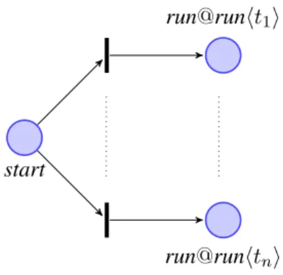
Initial transitions. A Creol program is defined by an initial configuration C0 composed of a set
of classes, a set of objects and an initial thread. We denote the initial thread with run. This is the main thread in the program, thus it is not called by another thread, does not belong to any object, nor class. Due to this lack of information, i.e. no object and method of the caller and no called object and method, we will use as abstract name for the initial thread the tuple run@run. As discussed above, we will define a way to extract from the thread code a set of abstract statement traces: let t1, . . . , tn
be such traces. Hence we can have different abstract representations in the Petri net for the initial thread: run@runht1i, . . . , run@runhtni. To activate nondeterministically one of them, we consider an
auxiliary place start, that will contain a token in the initial configuration, and n alternative transitions that move such token in one of these n places (see Fig. 2).
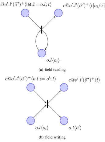
Method Calls. We present the Petri net transitions for a method call in Fig. 3. Depending on whether the result of the call will be assumed to be part of a deadlock or not, the created thread is tagged (see Fig. 3.a, notice the symbol “?”) or it is not (see Fig. 3.b). In the first case, the new thread will be abstractly named with [email protected]? (where c0 represents the caller) while in the second case with [email protected]. In both cases, the new thread will execute one of the traces t0 extracted from the definition of method l in the class of object o. More precisely, the Petri net will include two transitions, like those reported in Fig. 3, for each trace t0obtained as abstraction of the Creol code of the l method definition.