HAL Id: hal-01369787
https://hal.archives-ouvertes.fr/hal-01369787
Submitted on 21 Sep 2016
HAL is a multi-disciplinary open access
archive for the deposit and dissemination of
sci-entific research documents, whether they are
pub-lished or not. The documents may come from
teaching and research institutions in France or
abroad, or from public or private research centers.
L’archive ouverte pluridisciplinaire HAL, est
destinée au dépôt et à la diffusion de documents
scientifiques de niveau recherche, publiés ou non,
émanant des établissements d’enseignement et de
recherche français ou étrangers, des laboratoires
publics ou privés.
Zones in Circum-Saharan Africa Using Monthly
Dynamics of Multiple Indicators
Didier Leibovici, Gilbert Quillevere, Jean-Christophe Desconnets
To cite this version:
Didier Leibovici, Gilbert Quillevere, Jean-Christophe Desconnets. A Method to Classify Ecoclimatic
Arid and Semi-Arid Zones in Circum-Saharan Africa Using Monthly Dynamics of Multiple
Indica-tors. IEEE Transactions on Geoscience and Remote Sensing, Institute of Electrical and Electronics
Engineers, 2007, 12 (45), pp.4000-4007. �hal-01369787�
A Method to Classify Ecoclimatic Arid and
Semi-Arid Zones in Circum-Saharan Africa Using
Monthly Dynamics of Multiple Indicators
Didier Leibovici, Gilbert Quillevere Jean-Christophe Desconnets
Abstract—Within the context of monitoring desertification using a network of observatories, one faces the problem of the representativeness of biophysical, ecological and socio-economical variations. Ideally one would choose at least one observatory for each homogeneous zone, using indicators that capture these variations. Here we focused only on ecoclimatic aspects defined by the global physical and climatic conditions characterising arid and semi-arid zones. The challenging aim of this paper is to spatially identify the different patterns of ecoclimatic variations. For most of the indicators of arid or semi-arid zones, temporal characteristics and interactions through a typical year are observed. In order to take into account these dynamics in the clustering approach one must use a methodology that captures interactions between spatial location, time of measurement and indicator measured. For this purpose a multiway analysis, gen-eralising PCA (Principal Component Analysis), has been used on internationally recognised ecoclimatic indicators [1], [2] that characterise arid and semi-arid zones. Most of these indicators were used non-dynamically or qualitatively to approve and certify observatories of the ROSELT network (R´eseau d’Observatoires pour le Suivi Ecologique `a Long Termes) [3]. A direct application of this method would be to assess homogeneity and validity of ecoclimatic characteristics for each observatory comparatively to its regional location within its country or within the whole circum-Saharan region.
Index Terms—Ecoregion, Ecoclimatic, arid zone, semi-arid zone, desertification, classification, Pattern Recognition, Multi-way analysis, Tensor decomposition, PTAk
I. INTRODUCTION
The UNCCD (United Nations Consortium to Combat De-sertification) defines desertification as: “Land degradation in arid, semi-arid and dry sub-humid areas resulting from various factors, including climate variations and human activities” [4]. In line with this definition and to better understand the process of desertification, the ROSELT (R´eseau d’Observatoires pour le Suivi Ecologique `a Long Termes) network of observatories for long term ecological monitoring was established in 1995 by OSS (Observatoire du Sahara et du Sahel, located in Tunis) whilst led scientifically by the IRD (Institut de Recherche pour le Developpement) unit IRD-US166 D´esertification. A process of approval and certification for each potential observatory was
Dr Didier Leibovici is with the Centre for Geospatial Sciences, Uni-versity of Nottingham, Nottingham NG7 2RD, United Kingdom, E-mail: Didier.Leibovici@nottingham.ac.uk
Gilbert Quilevere is with the IRD-US166 D´esertification, Maison de la T´el´ed´etection, 500 av JF Breton, 34093 Montpellier cedex 05, France, E-mail: gil.quillevere@mfr.asso.fr
Dr Jean-Christophe Desconnets is with the IRD-US166 D´esertification, Maison de la T´el´ed´etection, 500 av JF Breton, 34093 Montpellier cedex 05, France, E-mail: jcd@teledetection.fr
the beginning of building this network; it used internationally recognised ecoclimatic criteria to do so [2], [3] amongst other criteria, such as the history of scientific studies and institutional logistics. Beyond this approval procedure one can question the representativeness of the region covered by the network. This is very important given the goals of assessing the desertification processes in the circum-Saharan zone. Indirectly, homogeneity of conditions of each obser-vatory ensures easier analysis and comparisons within the network. In order to fulfil these objectives it is important to determine a fine enough pattern of classification of the studied region in ecoregions encompassing the biophysical, ecological, and socio-economical dynamical traits at a desired scale and resolution.
In this paper we focus only on ecoclimatic variations defined by the global physical and climatic conditions characterising arid, semi-arid and dry sub-humid zones. Our purpose is to describe a method to identify spatially the different patterns of ecoclimatic spatio-temporal variation. Relationships have been identified between rainfall, temperature and evapotran-spiration, for example to compute the length of dry season and to discriminate bioclimatic zones [1]. Some of these relations were already used in the ROSELT approval process and our aim here is to propose a means to enhance the classification process by taking into account the full monthly dynamics of some indicators.
After describing the indicator variables used for this analy-sis, we will explain the two steps of statistical methodology. The results will be discussed in comparison with some other ecoclimatic zonations coming from the initial ROSELT certi-fication process or the LGP (Length of Growing Period) used in the zoning methodology Global-Agro-Ecological-Zone of the FAO [5].
II. ARID AND SEMI-ARID ZONES INDICATORS
The indicators characterising arid and semi-arid zones used for the pattern recognition methodology are described in more details in [1], [2], [6], [7]. The aridity index, the ratio P/ET o [6] where P is the annual rainfall and ET o is the annual potential evapotranspiration of Penman-Monteith is the main indicator used in many research communities but with some small differences in thresholds [1]: on average a gradient of arid, semi-arid, and dry sub-humid P/ET o has values of 0.10, 0.35 and 0.50 but authors give different ranges of lower and higher values around these numbers. The ratio of monthly
averages, Pm m was kept in the analysis described later
as well as some other related and correlated indexes such as the Q3 index [7] expressing a ratio of the rainfall to the temperature amplitude, and the Pm < 2Tave criterion
identifying dry months. The number of dry months using Pm/ET om < 0.35 was also taken for comparison. Monthly
versions of these indicators were used as described in Table I. Some of these criteria were used in the approval selection procedure of ROSELT observatories [3] in terms of bioclimatic domain, according to a qualitative hierarchical procedure: latitude of location, aridity level and rainfall regime. For validation purposes the approach is sufficient, but to study the representativeness of the whole network relatively to the circum-Saharan zone, a geographical zonation using these indicators is necessary. To identify bioclimatic or ecoclimatic
TABLE I
THE10INDICATOR VARIABLES USED IN THE ANALYSIS Indicators Description
Pm monthly rainfall (mm)
Tmax monthly maximum of temperature(°C)
Tmin monthly minimum of temperature(°C)
Tave monthly average of temperature (°C)
ET om monthly potential evapotranspiration
of Penman-Monteith (mm) Pm/ET om monthly aridity index
Altave average altitude for the pixel grid considered(m)
dM 2Tnb number of of dry months according to the
criterion Pm< 2Tave
Q3m monthly simplified Emberger’s pluviothermal index Q3
Q3m= 3.43Pm/(Tmax− Tmin) (mm.°C−1)
dM ET onb number of of dry months according to
the criterion Pm/ET om< 0.35
patterns we propose to analyse the spatial distribution of the indicators mentioned above, on their monthly basis in order to consider annual dynamics. If some parameters do not vary in time (e.g. Altitude) their influence in the spatio-temporal dynamics of other parameters may be important to take into account.
III. CLUSTERING THE DYNAMICS OF MULTIPLE INDICATORS
Many sources to gather climatic data for this kind of study are listed in previous reports [8], [9] in which some technical points to prepare and manipulate all the data in the same format and resolution can also be found. The necessary climatic parameters were derived from the WORLDCLIM [10] database (1950-2000, see www.worldclim.org/current.htm for the most recent one) at resolution 5 arcmin (minutes of arc) i.e.approximately 0.08dd (decimal degree), and from the FAO for potential evapotranspiration of Penman-Monteith. All the parameters are monthly representatives of the 1950-2000 pe-riod, obtained in fact most likely by averaging over the 1960-1990 period and extended in some cases to the full period as described in [10]. This can be seen as ensuring large stability of the results under the approximation of ignoring inter-annual
variations, e.g. no climate change. For the studied area (Africa between latitudes 39.143 North and −5.731 South) at the chosen resolution, the data structure of the ecoclimatic profiles measured by the variables listed on Table I is a collection of 12 matrices (one for each month) of 10 variables (ecoclimatic profile) measured over 298249 spatial-locations (number of pixels).
One approach to cluster the annual dynamics of these indicators could be to perform a classic clustering method such as the k-means on the 120 variables or perform it after a Principal Component Analysis of them. Conceptually and technically this approach has some drawbacks. First of all some correlations across the year of different indicators may not be meaningful and the description of the resulting clustering may become difficult. Understanding the dynamic of indicators is better expressed using a method enabling the analysis of the interactions between measurement times, indicators measured and spatial-locations, a method seeing these as three different factors playing an equivalent role in the ecoclimatic dynamic description. Expressing differences in ecoclimatic zones in terms of seasonal patterns associated with specific indicators, such as monomodality or bimodality for ombrothermal diagrams, for example, derives from such approaches.
A. Capturing the dynamics features
The first part of this section describes a methodology that allows analysis and synthesis or extraction of interactions between the factors spatial-locations, months and indicators measured. The second part will illustrate the results. The method is taking advantage of the tensorial structure of the data, a structure which expresses the multiway interaction. It can be considered as one generalisation of PCA for multi-array data: method PTAk [11] (Principal Tensor Analysis k-modes). It has been programmed as an R add-on package [12]; an extensive description of the package is also available [13]. PTAk offers a decomposition similar to what is obtained from matrices with a Principal Component Analysis, but working on tensors, i.e. in mathematical algebra they are multilinear maps, seen here simply as multiple-entries tables (k entries). Algebra properties allow to derive multiple-entries table calculus as it does for matrix calculus. In our case there are three entries or data modes: spatial-location, month, indicator, and each cell of the table contains the value of one indicator for a given month at a specific location. In order to describe the generalisation proposed with the PTAk model, let us first rewrite the PCA method within a tensorial framework.
1) The PTAk method as an extension of PCA: For a given matrix X of dimension n × p, the first principal component is a linear combination (given by a p-dimensional vector ϕ1)
of the p columns ensuring maximum sum of squares of the coordinates of the n-dimensional vector obtained. The square root of this sum of square is called the first singular value σ1. One has:t(Xϕ1)Xϕ1= σ12 and Xϕ1/σ1 is the principal
written either in matrix form or tensor form: σ1 = max kψkn=1 kϕkp=1 (tψXϕ) = max kψkn=1 kϕkp=1 X..(ψ ⊗ ϕ) = tψ1Xϕ1= X..(ψ1⊗ ϕ1) (1) In equation 1 X is used either for the matrix or the tensor. An easy way of understanding computationally the operators “..” and “⊗” is to see them as the following operations: ψ1 ⊗ ϕ1 is a np vector of the n blocks of the p vectors
ψ1iϕ1, i = 1, ...n; “..” called a contraction generalises the
multiplication of a matrix by a vector and in the case like here of equal dimensions of the two tensors (np) corresponds to the natural scalar product (X is then also seen an np vector). ψ1is termed first principal component, ϕ1 first principal axis,
(ψ1⊗ ϕ1) is called first principal tensor. Now if X is a tensor
of higher order, say 3 here with the modes: time or month (t = 12),variable or indicator (v = 10) and space or spatial-location (s = 298249), we can look for the first principal tensor associated with the singular value with the optimisation form: σ1 = max kψks=1 kϕkv=1 kφkt=1 X..(ψ ⊗ ϕ ⊗ φ) = X..(ψ1⊗ ϕ1⊗ φ1) (2)
Adding an orthogonality constraint (projection onto the or-thogonal tensorial of the principal tensor, see equation 3) allows us to carry on the algorithm to find the second prin-cipal tensors and so on. Following the algorithm scheme, the decomposition obtained (for k-way data called P T Akmodes)
offers a way of synthesising the data according to uncorrelated sets of components ordered by the percent of total sum of squares. Within this algorithm scheme one can distinguish principal tensors from associated principal tensors. The latter are associated to a principal tensor as they show one or more component of this principal tensor in their sets of components. The associated principal tensors are obtained by a P T Ak−1-modes decomposition once the k-modes data has
been “contracted” by the given component. This makes the algorithm a recursive algorithm with the following procedure:
P T Ak(X) = σ1(ψ1⊗ ϕ1⊗ φ1) + ψ1⊗1P T Ak−1(P (ϕ⊥1 ⊗ φ⊥1)X..ψ1) + ϕ1⊗2P T Ak−1(P (ψ1⊥⊗ φ⊥1)X..ϕ1) + φ1⊗3P T Ak−1(P (ψ⊥1 ⊗ ϕ ⊥ 1)X..φ1) + P T Ak(P (ψ⊥1 ⊗ ϕ⊥1 ⊗ φ⊥1)X) (3)
The notation ⊗imeans that the vector on the left hand will take
the ith place, among the k places here, in each full tensorial product. More details on the properties of the method and on using the package is given in the references [11], [13]. As seen on Table II, in almost the same way as for PCA (equivalent to P T A2 modes) one gets a hierarchy of principal tensors (see
next section for decoding the names given on the first column)
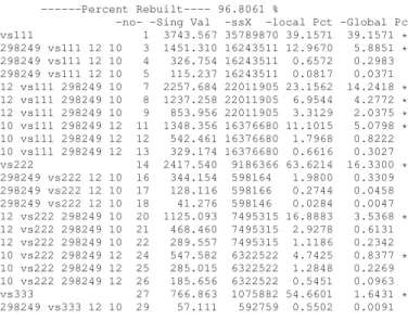
corresponding to a hierarchy of sum of squares, i.e. the singular values (σ) under the column -Sing Val associated to each principal tensor) squared. It is a multilevel hierarchy in agreement with the equation 3. Basically if the tensor is globally centred one gets a variance decomposition. Percents of variance explained associated to each Principal tensors can be used to retain main variability within the data tensor X. These percentages are in the -Global Pct column of Table II (-local Pct are relative to the sum of squares given in column -ssX linked to the current tensorial optimisation as defined in equation 3). Plots of the vector components of a particular principal tensor allows the description of the captured variability. For the ecoclimatic analysis one would read simultaneously a map configuration (spatial-location component), a annual pattern (month component) and an axis describing variables associations and oppositions (indicator component), together expressing the monthly dynamic of the ecoclimatic characteristics.
TABLE II
SUMMARY OF THEPTA3DECOMPOSITION(DOWN TO3PRINCIPAL TENSORS AND3ASSOCIATED PRINCIPAL TENSORS FOR EACH SUB-ANALYSIS)OF THE10ECOCLIMATIC INDICATORS MEASURED ON12
MONTHS(AVERAGE OVER50YEARS)-AT298249GRID PIXELS OF CIRCUM-SAHARA AND SAHARA ZONE. (*:SELECTED FOR KMEANS
ANALYSIS REPRESENTING93%)
PTA3 centred reduced on indicators ---Percent Rebuilt---- 96.8061 %
-no- -Sing Val -ssX -local Pct -Global Pct vs111 1 3743.567 35789870 39.1571 39.1571 * 298249 vs111 12 10 3 1451.310 16243511 12.9670 5.8851 * 298249 vs111 12 10 4 326.754 16243511 0.6572 0.2983 298249 vs111 12 10 5 115.237 16243511 0.0817 0.0371 12 vs111 298249 10 7 2257.684 22011905 23.1562 14.2418 * 12 vs111 298249 10 8 1237.258 22011905 6.9544 4.2772 * 12 vs111 298249 10 9 853.956 22011905 3.3129 2.0375 * 10 vs111 298249 12 11 1348.356 16376680 11.1015 5.0798 * 10 vs111 298249 12 12 542.461 16376680 1.7968 0.8222 10 vs111 298249 12 13 329.174 16376680 0.6616 0.3027 vs222 14 2417.540 9186366 63.6214 16.3300 * 298249 vs222 12 10 16 344.154 598164 1.9800 0.3309 298249 vs222 12 10 17 128.116 598166 0.2744 0.0458 298249 vs222 12 10 18 41.276 598146 0.0284 0.0047 12 vs222 298249 10 20 1125.093 7495315 16.8883 3.5368 * 12 vs222 298249 10 21 468.460 7495315 2.9278 0.6131 12 vs222 298249 10 22 289.557 7495315 1.1186 0.2342 10 vs222 298249 12 24 547.582 6322522 4.7425 0.8377 * 10 vs222 298249 12 25 285.015 6322522 1.2848 0.2269 10 vs222 298249 12 26 185.656 6322522 0.5451 0.0963 vs333 27 766.863 1075882 54.6601 1.6431 * 298249 vs333 12 10 29 57.111 592759 0.5502 0.0091 ...
2) Ecoclimatic dynamics extracted: On Table II the de-composition has been done up to 96% of variability of the data which was centred and reduced along the indicator mode beforehand. The first column describes leading names of the principal tensors or associated principal tensors relatively to the singular values optimisation procedure, the second column identifying it. vs111 for example is the first singular value and represents the first principal tensor; 298249 vs111 12 10 represents the tensors obtained after contracting the data by the spatial-location component of the first principal tensor (vector of length 298249) i.e. X..ψ1, which here are obtained
by a P CA of a 12×10 matrix. The first solution on this P CA is removed from the list (also implicit in equation 3) as it is by construction exactly the components obtained on vs111 (the associated tensor would have been the -no- 2 on Table
II). To illustrate the kind of characterisation in terms of the
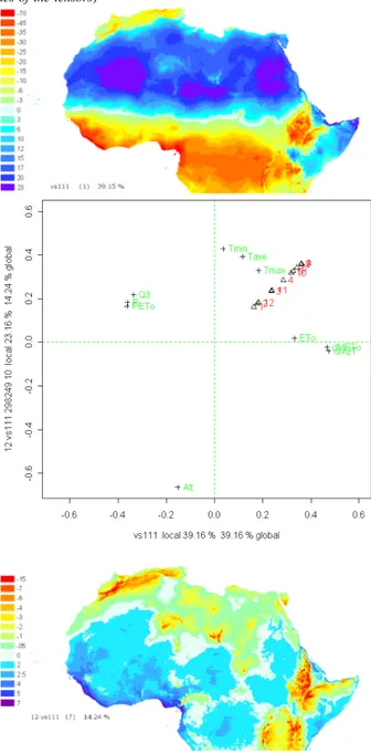
Fig. 1. Spatio-temporal association of ecoclimatic indicators captured in the first principal tensor representing 39.16%(vs111) and on the first month-mode associated principal tensor representing 14.25% of variability - see Table II -. ( Labels of indicators are the first letters of the names given in Table I; scatter plot and spatial values are the “loadings” or components values of the tensors)
patterns of interactions between spatial-location, month and indicator, it is interesting to look at Figures 1 and 2.
On Figure 1 we have the plots of components of two different tensors. The month and indicator modes are plotted on the same scatter plot and their spatial-location mode component can be read simultaneously to explain the vari-ability captured. For the tensor n°1 (vs111) one can see a spatial separation between the Saharan zone positively weighted, with North Maghreb, Sahelian zone and central Africa negatively weighted. Apart from the area in Somalia, this appears mainly as a double latitude gradient North and
South from the Sahara. This is associated with the opposition on one side of drought and extreme dry condition indicators (ET om, dM 2Tnb, dM ET onb, Tmax) and on the other side
rain related indicators (Q3m, Pm, P ET om) ; and this occurs
all year around, and especially during rainy seasons -May(5) to October(10)-. The vertical axis on Figure 1 shows an opposition between Altitude and temperature (T min more strongly) also persistent all year and more likely during rainy seasons -May(5) to October(10)-. Principal Tensor n°7 is associated to Principal Tensor n°1 along the month-mode, so it has the same month component vector. This vertical axis is read with the bottom spatial picture showing high relief correlated with it. We presented two other tensors on Figure
Fig. 2. Spatio-temporal association of ecoclimatic indicators captured in the second and third principal tensors representing 16.33% and 1.64%of variability - see Table II -. (Labels of indicators are the first letters of the names given in Table I; scatter plot and spatial values are the “loadings” or components values of the tensors)
2, respectively the second and third principal tensors (vs222 and vs333). The month and indicator modes plot shows an
association of T emperature and the months (December(12), January(1) and February(2)) (i.e dry months for the tropical zone) which is, for the vs222 tensor, linked with potential evapotranspiration ET om and a gradient North-South for the
whole Maghreb opposed to low land oceanic zones centered in Gabon and in Somalia. This same association also exists slightly on tensor vs333 but also for July(7), August(8) and September(9), then associated with Altitude and opposed to the whole Sudan-Sahel zone (beyond the traditional semi-arid zone) linked mainly with the semi-aridity index (P ET om),
pluviothermal index (Q3m), number of dry months (dM 2Tnb
and dM ET onb) but also rainfall (Pm) and that for mid-season
months. Note the month pattern on one axis opposing the extreme season months to mid-season ones and on the vs222 opposing dry hot months to wet hot months.
B. Ecoclimatic zones and their proximities
Once meaningful Principal Tensors are selected using both quantitatively the breakdown of variability given in the print-out in Table II and qualitatively the plots of components, it is possible to perform a multivariate clustering on the corresponding spatial-location components to obtain spatial classes of zones with similar ecoclimatic monthly dynamics. We used a simple k-means procedure with a chosen number of 15 classes. In order to minimise the influence of random starts, we used as starting points a parametric estimation of the (k-means) cluster means via 15 principal points [14] using the algorithm of T. Tarpey [15]. On a few tries the average persistence accuracy among the 15 classes was around 92%. Some descriptive statistics of the indicators would give a summary of the meaning of a particular class. In this paper we are focussing more on the spatial properties of the obtained classes. As a matter of fact it is also possible to perform another P T A3 on say the cluster means (centroids) of each class in order to characterise the different montly dynamics of the indicators which would be useful for description of the physical processes associated.
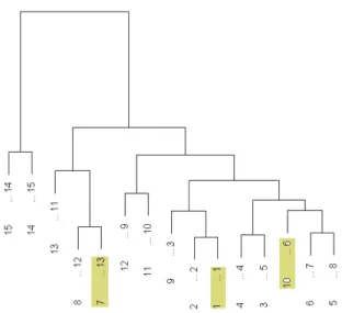
In order to reinforce the ecoclimatic proximity of the classes obtained we performed a hierarchical clustering on the centroids of the classes. The dendogram obtained, expressing a “pseudo distance ordering” of the classes, is used to calibrate the colour range on Figure 4, i.e. one colour for each class and the class number depending on its position in the dendogram. Two different ways of defining a pseudo order of the classes has been used. The first method uses directly the height of merging the groups, so the depth difference of colours express how similar a class is to another one in terms of level of merging (on Figure 3 the class numbers with the Height algorithm are at the bottom). It is not reasonable if for example two merging “events” happen on each side of the tree, i.e. these classes may merge together quite “late” in the tree. We corrected this aspect with a second partial ordering. The second algorithm, called To first on Figure 3 (class numbers on top), to build this pseudo-distance, postulates that the further you have to go back down to reach a reference class (one of the first aggregated, here class 1) means a higher distance. On Figure 3 the class 1 for example should be closer
Fig. 3. Partial orderings issued from the Complete linkage’s hierarchy of the 15 classes (obtained after kmeans clustering using selected principal tensors (spatial-location component) from P T A3 analysis): partial ordering according to height, partial ordering according to height and relative to the first merging ; hightlighted classes are discussed in the text.
to class 10 than class 7 (seen with Height algorithm). With the To First algorithm the last two classes numbers become respectively 6 and 13. This gives a compromise between merging heights and “distance” to previously merged classes. Working on the history of aggregation automatically allows the classes to be ranked for each chosen pseudo-order. The colour scale of the map of ecoclimatic regions will be done using the second algorithm for the order numbering of classes. When looking at representativeness one would be concerned in the chosen number of classes. This was done on the basis of the number of classes already existing in other zonation of Africa [5], [16]. In a multilevel zonation approach the methodology presented here could be made more flexible on the choice of number of classes by performing the k-means algorithm on a higher number of classes, say 50 and then reducing this number in cutting the tree after the hierarchical clustering on the centroids of the classes. Another type of representativeness is linked with validity and for this purpose comparisons with other existing classifications has to be addressed.
Fig. 4. Ecoclimatic Classes with their aggregation tree illustrating hier-archical climatic proximities (based on WorldClim 2004 parameters) and 34 ROSELT pilots observatories polygons (Egypt(2), Tunisia(3), Algeria(5), Morocco(3), Mauritania(3), Cap-Verde(2), Senegal(3), Mali(3), Niger(4), Kenya(4), Ethiopia(2)).
IV. ECOCLIMATIC REPRESENTATIVENESS OFROSELT The approach is complementary to an approval process but can also be seen as a reverse approach, as instead of validating a specific location independently of the national or regional mosaic of ecoclimatic zones, it builds the desired mosaic of ecoclimatic pattern. This pattern can be used to locate new observatories or assess validity in terms of ecoclimatic charac-teristics relative to the different patterns encountered within a
wider zone: representativeness. Qualitative representativeness can be assessed by using a description of classes relative to their dynamics throughout the year and by analysing the physical distribution of the observatories. Figure 4 illustrates a qualitative assessment of ROSELT representativeness in term of ecoclimatic variations of the circum-saharan zone. The 32 observatories covered nearly all the classes under arid, semi-arid, and dry sub-humid regions, i.e the ROSELT zone (defined above, II). The class 7 borderline of the dry sub-humid zone is not represented within the network. Note the classes 6, 12, 13, 14 and 15 are not in the ROSELT zone (not shown on figure 4). The observatories are more likely to represent one class each: homogeneity criterion. Only 1/3 of the observatories are of two classes with their main class ranging from 60-99% of their area but in fact only half of them had their main class below 80% of their area.
This methodology can also be applied at national level in order to establish a framework for positioning relevant observatories, for example by keeping each observatory more homogeneous. Results of this methodology applied also at national level are included in the www.ROSELT-OSS.org website in a numerical Atlas [9] available within the metadata catalogue of the network [17], [18].
A. Comparison with other pattern zonation method
Other zonation systems of Africa exist together with avail-able databases GAEZ-2000 (Global Agro-Ecological Zones) [5], ACMAD (African Center of Meteorological Applications for Development) [16] or ANUCLIM (Australian National University CLIMatic data) [19] to name a few. Most of these ecoregions are nonetheless made at world or continental level. Some zones considered here are not especially related to circum-sahara as well but few extra zones help calibrating what has been obtained.
For a fine climate pattern classification, 15 classes may appear rather small in comparison with some 252 theoretical ones and in fact 200 of them found by Le Hou´erou et al. [20]. Unfortunately no numerical map of Le Hou´erou full classifi-cation was available for direct spatial comparison. The method used in his paper could deal with a higher number of clusters but it may be at the price of losing simplicity. In GAEZ-2000 one major criterion is the LGP (Length of Growing Period) which is certainly well correlated with climatic data and may be better than the number of dry months. It is also very interesting that the spatial coherence and homogeneity is well achieved with the herein method without any spatial constraint other than actual indicator measurements natural spatial autocorrelation.
Considering climatic variations alone can be rather limiting and like other ecoregion pattern methodology, we combined our climatic pattern clustering with other factors: soil, veg-etation and human related pressure. Some of these results that allows complete representativeness analysis have been reported in [8]. In an excellent recent review of multivariate ecoregion methods [21] the multilayer or multifactor aspects was also emphasised either within the clustering methods or for visualisation issues with a very powerful Red, Green, Blue
combination according to three different factors, e.g. water balance, soil, and climatic characteristics coming from three PCA. If some methods combine the spatial, environmental parameters and time domains for the observations they are rarely considered as a three-way interaction within the statis-tical methodology which we addressed here.
V. PERSPECTIVES ANDCONCLUSION
The purpose of the paper was to demonstrate the use of a method to identify ecoclimatic patterns, rather than explaining the physical process of them, which is nonetheless very important when dealing with desertification characterization. A full description of each class would be necessary followed by a validation of physical process associated with each description. As ever, different methods should be compared also on the basis of the results obtained, this is a matter of a full different paper more appropriate in the field biometeorology as suggested by one reviewer.
The method proposed allows validity and homogeneity assessment of ecoclimatic characteristics for each observa-tory but also representativity analysis of the network. The results are very encouraging but some issues may be relevant depending on the use of this classification. Fuzziness of the borders can be addressed when dealing with ecoregion borders and some methods could be applied a posteriori [22], [23]. Other fuzzy algorithms are available but the intensive computing needed for this massive dataset may preclude their use. Averaging over 50 years [10] for stability of results could be compared with an approach considering stable periods within these 50 years different. Taking into account relative evolutionary steps in the zonation from ecoclimatic charac-terisation, would now consider adding a period mode and a tensor of order 4 to analyse by a PTA4. The ecoclimatic dynamics would be described in terms of interactions between periods, months, ecoclimatic indicators and spatial-locations. Identifying these periods say for example before 1970 and after, could be useful in terms of climate change analysis and its impact on the changes in the pattern of spatial distributions. The method described in this paper could be applied directly to a collection of remote sensing data expressing some multi-variate monitoring aspects which then could also benefit from remote sensing clustering methodology about spatial and/or temporal constraints such as in [24] using geostatistics or in [25] using multispectral spatial clustering. The methodological approach of the paper could be applied on vegetation charac-teristics and on some socio-economic indicators in order to build ecoregions of the circum-Saharan area incorporating the spatio-temporal dynamic of all the parameters involved. This zonation would then constitute a basis for better understanding of the regional desertification trends using sets of indicators obtained at local scale.
Acknowledgments
The authors whishes to thank Henry No¨el Le Hou´erou who showed a stimulating interest in this work and for helpful comments about the report [8]. Warm thanks go also to H´el`ene Fonta who finalised an atlas [9] available online within
http://mdweb.roselt-oss.org and containing maps issued from this methodology also at National levels.
REFERENCES
[1] H. N. Le Hou´erou, “An Agro-bioclimatic Classification of Arid and Semi-arid lands in the Isoclimatic Mediterranean Zones,” Arid Land Research and Management, vol. 18, pp. 301–346, 2004.
[2] ——, “Classification ´ecoclimatique des zones arides (s.l.) de l’Afrique du nord,” Ecologia Mediterranea, vol. XV (3/4), pp. 95–143, 1989. [3] ROSELT/OSS, Conception, organisation et mise en oeuvre de ROSELT,
ser. Collection ROSELT/OSS, IRD US166 D´esertification, Montpellier, 1995, vol. Document Scientifique n°1, 130p.
[4] UNCCD, “United Nations Convention to Combat Deser-tification from resolution 47/188 1992 ,” United Nations, http://www.unccd.int/convention/text/convention.php, UN convention, 1994.
[5] FAO, “FAOCLIM - User’s manual: A CD-ROM with World-wide Agroclimatic Database,” FAO (Food and Agriculture Organisation of the United Nations), Rome, http://www.iiasa.ac.at/Research/LUC/GAEZ/index.htm, Agrometeo-rology Series Working Paper No. 11, 1995.
[6] R. G. Allen, L. S. Pereira, D. Raes, and M. Smith, “ Crop Evap-otranspiration. Guidelines for Computing Crop Water Requirements.” FAO (Food and Agriculture Organisation of the United Nations), Rome, Irrigation and Drainage Paper, 1998.
[7] H. N. Le Hou´erou, The Isoclimatic Mediterranean Biomes, Bioclimatol-ogy, Diversity and Phytogeography, copymania ed., Montpellier, 2005, vol. 1 and 2, 765 ppp.
[8] G. Quillevere, “Representativit´e circum-saharienne du r´eseau d’observatoires ROSELT,” Maison de la T´el´ed´etection, Mast`ere SILAT (ENGREF-ENSAM-INA PG-ENSG), Montpellier, 2004. [9] H. Fonta, “Cr´eation d’une base de donn´ees g´eographique r´egionale
dans le cadre du programme ROSELT,” Maison de la T´el´ed´etection, m´emoire de D.U Cartographie des territoires et Syst`emes d’Information G´eographique Universit´e Montpellier III, 2005.
[10] R. Hijmans, S. Cameron, J. Parra, P. Jones, and A. Jarvis, “Very high resolution interpolated climate surfaces for global land area,” International Journal of Climatology, vol. 25, pp. 1965–1978, 2005. [11] D. Leibovici and R. Sabatier, “A Singular Value Decomposition of
k-Way Array for a Principal Component Analysis of Multiway Data, PTA-k,” Linear Algebra and Its Applications, vol. 269, pp. 307–329, 1998. [12] D. Leibovici, “PTA-k add on R-package version 1.1-12,” http:// cran.
r-project.org/ src/ contrib/ PACKAGES.html, vol. version 1.1-12, 2004. [13] ——, “An R-package for a generalisation of PCA to multiway data:
PTA-kmodes.” Journal of Statistical Software, vol. in preparation, 2007. [14] B. Flury, “Principal Points,” Biometrika, vol. 77, pp. 33–41, 1990. [15] T. Tarpey, “A Parametric k-Means Algorithm,” Computational Statistics,
vol. to appear, 2006.
[16] M. Magdy Kamal and B. Beshay, “Atlas climatologique de l’afrique,” African Center of Meteorological Applications for De-velopment, http://medias.obs-mip.fr/acmad/fr/cahpf/cdomain.html, Tech. Rep., 1999.
[17] J. Desconnets, “MDweb, outil de catalogage et de localisation au service de l’environnement. Retour d’exp´erience dans le domaine des GIZC (programme Syscolag),” in Normalisation, M´etadonn´ees et Cata-logage. Aix en provence: Journ´ees Techniques du CRIGE-PACA, 2006, http://www.crige-paca.org/frontblocks/animation/animations.asp. [18] P. Boisson, S. Clerc, J. Desconnets, and T. Libourel, “Using a semantic
approach for a cataloguing service,” in OTM 2006 Workshops Part II, Springer, Ed. SeBGIS, 2006, pp. 1712 – 1722.
[19] J. P. McMahon, M. F. Hutchinson, H. A. Nix, and K. D. Ord, “ANUCLIM User’s Guide,” Centre for Resource and Environmental Studies, Australian National University, Canberra., http://cres.anu.edu.au/outputs/africa.php, Draft Report, 1995.
[20] H. N. Le Hou´erou, G. F. PoPov, and L. See, “Agro-bioclimatic clas-sification of Africa.” FAO (Food and Agriculture Organisation of the United Nations), Rome, FAO Agrometeorology Working Paper, 1993. [21] W. W. Hargrove and F. M. Hoffman, “Potential of multivariate
quan-titative methods for delineation and visualization of ecoregions,” EN-VIRONMENTAL MANAGEMENT, vol. 34, no. Suppl.1, pp. S39–S60, 2004.
[22] ——, “Using multivariate clustering to characterize ecoregion borders,” Computers in Science and Engineering Special Issue on Scientific Visualization of Massive Data Sets, vol. 1, no. 4, pp. 18–25, 1999.
[23] ——, “Representativeness and network site analysis based on quanti-tative ecoregions,” Oak Ridge National Laboratory Environmental Sci-ences Division, http://research.esd.ornl.gov/ hnw/network/, web, 2002. [24] A. Boucher, K. C. Seto, and A. G. Journel, “A Novel Method for
Mapping Land Cover Changes: Incorporating Time and Space With Geostatistics,” IEEE Transactions on Geoscience and Remote Sensing, vol. 44, no. 11, pp. 3427–3435, November 2006.
[25] L. O. Jimenez, J. L. Rivera-Medina, E. Rodriguez-Diaz, E. Arzuaga-Cruz, and M. Ramirez-Velez, “Integration of spatial and spectral in-formation by means of unsupervised extraction and classification for homogenous objects applied to multispectral and hyperspectral data,” IEEE Transactions on Geoscience and Remote Sensing, vol. 43, no. 4, pp. 844–851, April 2005.