HAL Id: hal-01128894
https://hal.archives-ouvertes.fr/hal-01128894
Submitted on 6 May 2021
HAL is a multi-disciplinary open access
archive for the deposit and dissemination of
sci-entific research documents, whether they are
pub-lished or not. The documents may come from
teaching and research institutions in France or
abroad, or from public or private research centers.
L’archive ouverte pluridisciplinaire HAL, est
destinée au dépôt et à la diffusion de documents
scientifiques de niveau recherche, publiés ou non,
émanant des établissements d’enseignement et de
recherche français ou étrangers, des laboratoires
publics ou privés.
The impact of different external sources of iron on the
global carbon cycle
Alessandro Tagliabue, Olivier Aumont, Laurent Bopp
To cite this version:
Alessandro Tagliabue, Olivier Aumont, Laurent Bopp. The impact of different external sources of iron
on the global carbon cycle. Geophysical Research Letters, American Geophysical Union, 2014, 41 (3),
pp.920-926. �10.1002/2013GL059059�. �hal-01128894�
The impact of different external sources
of iron on the global carbon cycle
Alessandro Tagliabue1, Olivier Aumont2, and Laurent Bopp3
1
Department of Earth, Ocean and Ecological Sciences, School of Environmental Sciences, University of Liverpool, Liverpool, UK,
2Laboratoire de Physique des Océans, Centre IRD de Bretagne, Plouzané, France,3Laboratoire des Sciences du Climat
et l’Environnment, CNRS-CEA-UVSQ, Gif sur Yvette, France
Abstract
Variable supply of iron to the ocean is often invoked to explain part of past changes in atmospheric CO2(CO2atm). Using model simulations, wefind that CO2atmis sensitive on the order of 15, 2, and 1 ppm to sedimentary, dust, and hydrothermal iron input. CO2atmis insensitive to dust because it is not the major iron input to the Southern Ocean. Modifications to the relative export of Si(OH)4to low latitudes are opposite to those predicted previously. Although hydrothermalism is the major control on the iron inventory in ~25% of the ocean, it remains restricted to the deep ocean, with minor effects on CO2atm. Nevertheless, uncertainties regarding the iron-binding ligand pool can have significant impacts on CO2atm. Ongoing expansion of iron observations as part of GEOTRACES will be invaluable in refining these results.1. Introduction
The role of the micronutrient iron (Fe) in governing phytoplankton primary productivity and the carbon cycle has become well established [e.g., Boyd and Ellwood, 2010]. By limiting phytoplankton growth in regions important for air-sea CO2transfer, Fe-mediated changes to export production have the potential to drive
significant changes in atmospheric CO2levels (CO2atm). Contemporary Fe limitation has resulted in unused,
macronutrient (NO3and PO4) stocks in the equatorial Pacific, subarctic Pacific, the north Atlantic, and, largest
of all, in the Southern Ocean. Crucial in the Fe cycle is the process of organic complexation [Gledhill and Buck, 2012], which retains Fe in the dissolved pool (DFe).
Early studies suggested CO2atmreductions of>70 ppm if macronutrients in the Southern Ocean were fully
de-pleted [Sarmiento and Orr, 1991], seemingly supportive of variations in dust supply of Fe-driving glacial-interglacial CO2atmfluctuations [Martin, 1990]. However, complete macronutrient depletion is rarely possible when the
direct effect of Fe is modeled due to other limiting factors (e.g., light and/or macronutrients) [Aumont and Bopp, 2006]. A recent review [Kohfeld and Ridgwell, 2009] reports changes in CO2atmbetween 5 and 20 ppm, with a
central estimate of 15 ppm in response to dust Fe fertilization. Changing Fe supply has also been proposed to impact CO2atmindirectly via the“silicic acid leakage” hypothesis [Matsumoto et al., 2002] that suggests greater
dust Fe supply during glacial periods would alleviate Fe limitation and reduce the silicification of diatoms. Greater Si(OH)4, relative to NO3, should then be transported to low latitudes, allowing diatoms to outcompete
resident calcifying plankton therein and the increase alkalinity lowers CO2atm[Matsumoto et al., 2002; Kohfeld
and Ridgwell, 2009]. Whether by directly or indirectly, variations in dust Fe supply are frequently invoked as a driver of CO2atmvariability [e.g., Lourantou et al., 2010; Martinez-Garcia et al., 2011; Ziegler et al., 2013]. Recently, sedimentary [e.g., Moore and Braucher, 2008; Tagliabue et al., 2009] and hydrothermal [Tagliabue et al., 2010] Fe sources have also been highlighted, and there are differences in the degree of Southern Ocean dust deposition [Huneeus et al., 2011]. Outstanding questions also remain regarding the role of iron-binding ligands in buffering the DFe pool [Gledhill and Buck, 2012] thereby modulating the biological impact. In this study, we use a state of the art ocean general circulation and biogeochemistry model with a number of different Fe sources and representations of Fe cycling to assess the impact on CO2atmduring long time scale simulations.
2. Methods
2.1. Biogeochemical Model
We use the latest version of the NEMO-PISCES model (v3.5, www.nemo-ocean.eu). Briefly, the biogeochemical component PISCES includes two phytoplankton functional types, two zooplankton, two particle size classes,five
Geophysical Research Letters
RESEARCH LETTER
10.1002/2013GL059059
Key Points:
• Atmospheric CO2is relatively insensi-tive to changes to dust supply of iron • Hydrothermal Fe is key to the iron in-ventory, but has a small effect on CO2 • There are unexpected changes to Si
cycling due to changes in Fe input
Supporting Information: • Readme • Text S1 • Figure S1 • Figure S2 • Figure S3 Correspondence to: A. Tagliabue, a.tagliabue@liverpool.ac.uk Citation:
Tagliabue, A., O. Aumont, and L. Bopp (2014), The impact of different external sources of iron on the global carbon cycle, Geophys. Res. Lett., 41, 920–926, doi:10.1002/2013GL059059. Received 23 DEC 2013 Accepted 14 JAN 2014
Accepted article online 17 JAN 2014 Published online 5 FEB 2014
limiting nutrients (NO3, PO4, DFe, NH4, and Si(OH)4), oxygen, dissolved inorganic carbon, dissolved
or-ganic carbon, alkalinity, calcite, and biogenic silica. The full carbon system is simulated [Aumont and Bopp, 2006], which permits the calculation of the ocean partial pressure of CO2 (pCO2) and associated
air-seafluxes. Fe is explicitly simulated in the dissolved pool, two particle fractions, and the biological compartments (since Fe uptake is considered independently). DFe is removed by scavenging, with free Fe explicitly calculated using afixed ligand concentration (0.6 nM) and conditional stability (1012M 1), alongside additional colloidal pumping DFe losses. Scavenging rates depend on particle concentrations and scavenged Fe is returned to DFe via dissolution. Modeled DFefields are compared to a recent observational compilation [Tagliabue et al., 2012] and other biogeochemical tracers are evaluated in the supporting information.
Concerning sources, PISCES accounts for the external DFe supply from dust, continental margin sedi-ments, hydrothermal vents, and rivers, with sea ice incorporation/release of dissolved Fe similar to Lancelot et al. [2009]. Dust supply is either from the INCA [Huneeus et al., 2011] or National Center for Atmospheric Research (NCAR) [Mahowald et al., 2005] models assuming constant solubility of 2%. Sedimentary input varies as a function of sediment oxygenation, itself a function of shelf depth [Middelburg et al., 1997] using high-resolution bathymetry [Aumont and Bopp, 2006]. Hydrothermal input is driven by ridge spreading rate [Tagliabue et al., 2010], increased to account for new observations [Saito et al., 2013]. The total DFeflux is 26.9 and 13.5 Gmol DFe from sediments and hydrothermalism, respectively, with a dust providing 32.7 or 37.5 Gmol DFe from the INCA or NCAR models, respectively. While the NCAR model only has slightly more total dust supply, it has a factor of 3.8 more south of 30°S, making these two dust models good candidates for exploring the CO2atmsensitivity to differing levels of
Southern Ocean dust input [Wagener et al., 2008].
2.2. Experimental Design
We spun up the model for 1000 years with dust from INCA (PISCES-INCA) and NCAR (PISCES-NCAR) and coupled to a well-mixed CO2atmreservoir (initialized with a preindustrial value of 280 ppm) that is adjusted
due to simulated air-seafluxes. After the spin up, the air-sea CO2flux drift was <4 × 10 5Pg C or <0.25%
and total annual ocean productivity, export production and air-sea CO2 exchange were similar at
~39, 7.1, and 0.013 Pg C, respectively, for PISCES-INCA and PISCES-NCAR. We then launched six separate simulations where dust, sediment, and hydrothermal Fe sources were each removed (plus a control) for both PISCES-INCA and PISCES-NCAR (see Table 1). To this initial set of simulations we conducted a further five where sediment and hydrothermal sources were both removed, ligand concentrations were halved or doubled, and sediment sources were eliminated in combination with halved or doubled ligand concentrations. To determine the net impact of these perturbations on CO2atm and ocean biogeochemistry, rather than the initial adjustment, all experiments were 300
years (by which time the drift in anomalous air-sea fluxes was negligible, supporting information).
Table 1. A Summary of the Model Experiments Conducted, the Dust Model Used, and the Change in Atmospheric CO2, Carbon Export, Input of Iron, and Average Preformed PO4That Resultsa
Simulation Dust Source ΔCO2atm(ppm) ΔCEX(Pg C yr 1) ΔFeIN(Gmol Fe) PO4PRE(mmol L 1) CTLINCA INCA 0 (280) 0 (7.10) 0 (72.8) 1.733 NODUSTINCA INCA +1.8 0.06 32.7 1.741 NOSEDINCA INCA +14.5 0.52 26.6 1.770 NOHYDINCA INCA +1.1 0.02 13.5 1.737 CTLNCAR NCAR 0 (280) 0 (7.14) 0 (77.6) 1.731 NODUSTNCAR NCAR +2.3 0.11 37.5 1.741 NOSEDNCAR NCAR +13.5 0.44 26.6 1.765 NOHYDNCAR NCAR +1.0 0.01 13.5 1.735 NOSEDHYDINCA INCA +14.5 0.52 40.1 1.770
DLIGINCA INCA 5.4 +0.15 0 1.716
HLIGINCA INCA +5.1 0.14 0 1.749
NOSEDHLIG-INCA INCA +18.2 0.63 26.6 1.780 NOSEDDLIG-INCA INCA +10.0 0.37 26.6 1.758
a
DLIG and HLIG refer to doubled and halved ligand concentrations, respectively. CTL refers to Control Simulation.
3. Results and Discussion
3.1. Carbon Cycle Impact of Different Iron Sources
CO2atmis most sensitive to removal of sedimentary, then dust andfinally hydrothermal inputs, with
sensi-tivity to the assumed dust model (Table 1). For PISCES-INCA, CO2atmrises by 14.5, 1.8, and 1.1 ppm when
sediment, dust, and hydrothermal Fe sources are removed. When PISCES-NCAR is used, CO2atmrises by 13.5, 2.3, and 1.0 ppm upon removal of sediment, dust, and hydrothermal Fe sources. The change in export pro-duction is closely tied to the CO2atmchanges (Table 1) by ~28 ppm CO2atmincrease per Pg C reduction in
export (R2= 0.988, n = 14). Removing both sediment and hydrothermal sources in PISCES-INCA raises CO2atm by 14.5 ppm (Table 1), slightly less than the sum of each effect (15.6 ppm). This arises because organic ligands introduce nonlinearity in the scaling of the iron inventory response [Tagliabue et al., 2010]. In all cases, changes in CO2atmand export scale well with the modifications to preformed PO4(Table 1).
Well-documented“downstream effects” of Fe-mediated changes in macronutrient consumption [e.g., Sarmiento et al., 2004; Tagliabue et al., 2008] cause a complex spatial response (Figure 1). For example, reduced export production in the Southern Ocean due to eliminated sediment Fe causes an increased supply of macronutrients to low latitudes that fuels export production in these non-Fe-limited waters (Figure 1). Accordingly, thefinal perturbation to export production is around two thirds of the imme-diate response that occurs over thefirst few years. The largest changes in export production are seen in the tropical Atlantic/North Pacific, offshore Southern Ocean/North Atlantic, and around Iceland/New Zealand/Japan/Southern Ocean in response to removing dust, sediment, and hydrothermal iron, re-spectively. Export anomalies in the Southern Ocean from dust are larger using PISCES-NCAR, in line with the greater approximately fourfold greater dust supply (Figure 1).
3.2. How Do Different Iron Sources Impact Nutrient Biogeochemistry?
In all cases, greater Fe limitation unsurprisingly led to increases in the amount of residual NO3, PO4, and Si (OH)4that can fuel additional production in adjacent but not Fe-limited regions. Interestingly however,
a)NODUSTINCA b)NOSEDINCA
c)NODUSTNCAR d)NOHYDINCA
Δ
Carbon Export (mmol m
-2
d
-1
)
Figure 1. The change in carbon export (mmol C m 2d 1) for each of the experimental runs. No sedimentary (NOSEDNCAR) and No hydrothermal (NOHYDNCAR) are virtually identical to NOSEDINCAand NOHYDINCAand are not shown.
proportionally more Si(OH)4is transported than NO3, as shown by the Si* tracer (Si(OH)4-NO3) [Sarmiento
et al., 2004, Figure 2]. Greater Fe limitation (e.g., due to lesser Fe input) is thought to reduce Si* from greater silicification [e.g., Hutchins and Bruland, 1998; Sarmiento et al., 2004], but ostensibly, this should enhance Si (OH)4consumption in our simulations and reduce Si*, which is opposite to our results (Figure 2). In our simulations, the relative silicification of diatoms increases due to greater Fe limitation, but their relative abundance declines, which causes less net Si(OH)4consumption, relative to NO3, overall. Thus, in terms of Si*,
wefind the impact of changing Fe limitation on the composition of the phytoplankton assemblage out-weighs the physiological impact. The Si* of waters exported northward is consistently greater in response to reduced Fe inputs, and the largest effects are seen in response to the largest perturbation in Southern Ocean Fe inputs (Figure 2).
Away from localized sources, the integrated DFe column inventory (∫Fe, Figure S1 in the supporting infor-mation) is most sensitive to sediment and hydrothermal inputs rather than dust (across both dust models). We examined the influence of each source, by calculating the Δ∫Fe for each of the simulations. When sedi-ment sources are removed,Δ∫Fe is ≤ 250 μmol Fe m 2almost everywhere, reaching as low as≤ 500 μmol Fe m 2near the Southern Ocean shelves. The anomalies in∫Fe due to removing hydrothermal Fe are re-stricted to ocean ridges in the Northern Hemisphere but become much more widespread in the Southern Hemisphere (up to≤ 500 μmol Fe m 2in the Pacific Sector of the Southern Ocean). In contrast, it is only in the tropical Atlantic and northwest Indian Ocean where dust anomalies are significant (for either dust model).
3.3. The Most Significant Iron Source?
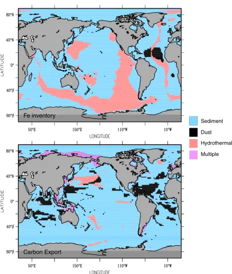
The relative role of different Fe sources in controlling certain properties of the system dependsfirstly on the property of interest and secondly on the assumptions regarding dust deposition. If we are concerned with ∫Fe, then sediment sources are most important for ~74% of the ocean area, followed by hydrothermal sources for ~23%, and dust for just ~2% (regardless of the dust model employed, Table 2). Hydrothermalism is most important in the eastern Pacific and the Pacific and Indian sectors of the Southern Ocean, with dust restricted to the tropical Atlantic and sediment sources dominating elsewhere (Figure 3). However, if we then turn our attention to carbon export, the picture changes slightly and despite sediment sources remaining dominant at 79–81% of the ocean area, dust is now more important at 12–16% and hydrothermalism is less important at
0 1000 2000 3000 4000 5000 0 1000 2000 3000 4000 5000 0 1000 2000 3000 4000 5000 0 1000 2000 3000 4000 5000 85S 75S 65S 55S 45S 20S 0 20N 40N 60N 80N 85S 75S 65S 55S 45S 20S 0 20N 40N 60N 80N 85S 75S 65S 55S 45S 20S 0 20N 40N 60N 80N 85S 75S 65S 55S 45S 20S 0 20N 40N 60N 80N
a)NODUSTINCA b)NOSEDINCA
c) NODUSTNCAR d)NOHYDINCA
Figure 2. The zonal mean change in Si* (Si(OH)4-NO3) (mmol m 3) for each of the experimental runs. Between 90°N and 40°S results are zonally averaged in the Atlantic Basin, while south of 40°S the zonal average is circumpolar. NOSEDNCARand NOHYDNCARare virtually identical to NOSEDINCAand NOHYDINCAand are not shown.
~3%. (Table 2 and Figure 3, depending on the dust model used). Hydrothermal control of export production is restricted to areas adjacent to shallow sources (near Iceland and Japan) or localized upwelling, with the influence of dust apparent in parts of the Pacific and Indian Oceans. In 3% of the ocean area (always on the shelf) more than one Fe source exerts equal control. The relative impact of a given source on CO2atmis regulated by its control on
export production. This is not surprising given the extent to which CO2atm
anom-alies are driven by changes in global carbon export (section 3.1). Less clear is the relationship between the extent to which a given source regulates∫Fe and CO2atm. A good example in this context is hydrothermal input,
which controls∫Fe over almost 25% of the ocean (Table 2) but contributes little to CO2atm(Table 1). Conversely, dust input regulates∫Fe over only ~2% of the ocean but contributes slightly more to CO2atm.
These results highlight the role of ocean ventilation and organic ligands (see section 3.4) in regulating
Figure 3. The source of Fe that dominates the anomalies in the column integrated (top) Fe inventory and (bottom) carbon export. Table 2. A Summary of the Relative Role Played by Different Iron
Sources in Governing the Column Inventory of Fe (∫Fe) and Carbon Export at 100 m (in Percent of Ocean Surface Area) Across the Range of Experimentsa
Dominant
Iron Source Dust Source
Driver of Anomalies (% Ocean Area) ∫Fe Carbon Export
Dust INCA 2.0 12.4 Sediment INCA 74.4 81.3 Hydrothermal INCA 23.6 3.2 Multiple INCA 0 3.1 Dust NCAR 2.6 15.9 Sediment NCAR 74.3 78.8 Hydrothermal NCAR 23.1 2.2 Multiple NCAR 0 3.1
the sensitivity of export production to subsurface Fe sources. Hydrothermal input is clearly a major control on the interior distributions of dissolved Fe but relies on deepwater ventilation for this Fe to be transported to the surface dwelling biota [Tagliabue et al., 2010]. Far from sources, organic ligands might act to stabilize the Fe inventory and thus buffer the impact of Fe input variability. In contrast, dust supply of Fe arrives directly at the surface and does not require physical processes to modulate its transfer to the biota.
3.4. Uncertainties in Iron Cycling
Varying our assumptions regarding the concentrations of DFe-binding ligands has significant impacts on CO2atm. For example, simply halving or doubling the ligand concentration (from 0.3 to 1.2 nM) modifies CO2atmby 5.1 or +5.4 ppm (Table 1), which is greater than the dust or hydrothermal effects. Taken in
combination with changing Fe inputs, modifying ligand concentrations can either accentuate or dampen the previously seen impact. For example, halving or doubling ligand concentrations alongside removing sedimentary Fe input modifies CO2atmby +10.0 or +18.2 ppm, respectively, compared to +14.5 ppm when ligand concentrations were not modified (Table 1). Overall, the effects of parallel ligand variations introduce additional changes on the order of 10–25%. The ligand scenarios we have examined remain well within the concentrations observed (e.g., 0.1 to> 2nM) [Gledhill and Buck, 2012], thereby highlighting the importance of organic complexation to the Fe inventory and CO2atm.
4. Future Considerations
4.1. Modifications to Atmospheric CO2
Reduced dust deposition of iron seen as a driver of the rise in CO2atmfrom glacial to interglacial epochs
[Lourantou et al., 2010; Martinez-Garcia et al., 2011; Ziegler et al., 2013]. This is at odds with ourfindings that the CO2atmsensitivity to dust iron to be of the order of ~ 2 ppm (Table 1). This arises because, while dust input
was the dominant Fe source in our simulations (Table 1), it is not the major regulator of export production in the Southern Ocean, which plays the dominant role in regulating CO2atm. Focus on constraining the glacial Fe
supply to the Southern Ocean is thus important in this regard. Moreover, changes to ligand concentrations can have a larger impact than dust and substantial uncertainties exist in constraining their cycling [Gledhill and Buck, 2012].
The concept that relative Si(OH)4export from the Southern Ocean to low latitudes is positively related to
Southern Ocean Fe supply due to varying silicification [Matsumoto et al., 2002] is not supported (Figure 2). We find that the relative amount of diatoms, rather than their degree of silicification, is dominant in regulating the relative export of Si(OH)4. Diatoms become less competitive as the Fe input is decreased and relatively
greater Si(OH)4is exported with reduced iron input to the Southern Ocean (Figure 2). Thus silicic acid leakage
may work against the general CO2atmtendency rather than being a driver of it. 4.2. Characterizing Iron Sources
A number of simplifying assumptions in our representations of the Fe inputs to the ocean could be improved in the future to yield more robust determinations of their relative role in regulating CO2atmand∫Fe. For
ex-ample, accounting for dust mineralogy and associated variability in Fe content/solubility should be addressed, although this will conceivably have a greater impact on local biogeochemistry and∫Fe than on CO2atm. In addition, recent work has highlighted variability in sediment [Homoky et al., 2013] and
hydro-thermal [Saito et al., 2013] inputs that would be important to constrain in future models. Our prior under-standing, and its inclusion in our model, was that shelf depth, and in particular, the degree of carbon oxidation was the main driver of Fe efflux [Elrod et al., 2004]. However, Homoky et al. [2013] have noted that some shelves can be less important sources of Fe than their depth and oxygen content would indicate. In a similar fashion, we assume that the hydrothermal Feflux is regulated by ridge spreading rate, as parameterized by a constant DFe/Helium ratio [Tagliabue et al., 2010]. Yet recent observations [Saito et al., 2013] suggest that there might be less variability in Fe input from hydrothermal vents than there is for helium. To respond to this, we have upscaled the DFe/Helium ratio in this study, but the connection to ridge spreading rate remains. All sources clearly also do not only supply DFe, and although our model simulates particulate Fe, we do not consider unique sources of particulate Fe. More observational and specific modeling work is therefore needed to better understand how shelf depth and other factors interact to regulate sedimentary Fe input and how
the local conditions of different hydrothermal systems regulate the dissolved Fe input distinctly to that of Helium. The ongoing expansion of Fe observations as part of the GEOTRACES project will prove invaluable in this regard.
5. Conclusions
We have quantified the CO2atmsensitivity to Fe supply from dust, sediments, and hydrothermal vents using two different representations of dust supply that differ by a factor of ~4 in their Southern Ocean deposition. Wefind CO2atmto be most sensitive to sediment iron supply, with a relatively weak sensitivity to either
representation of dust deposition or hydrothermal input. This arises due to the overwhelming role for sediment supply in regulating Southern Ocean export production. While hydrothermal input is crucial in governing the Fe inventory for ~25% of the ocean, its impact on export production and CO2atmis regulated
by ocean ventilation. Changing Fe supply to the ocean modifies the relative export of Si(OH)4to low latitudes,
but wefind that Si(OH)4export rises when Fe supply is reduced due to lesser diatom productivity, contrary to
the silicic acid leakage hypothesis [Matsumoto et al., 2002]. Interestingly, wefind that modifying assumptions regarding the concentration of ligands has a potentially very large effect on CO2atm, particularly in combi-nation with Fe source changes.
References
Aumont, O., and L. Bopp (2006), Globalizing results from ocean in situ iron fertilization studies, Global Biogeochem. Cycles, 20, GB2017, doi:10.1029/2005GB002591.
Boyd, P. W., and M. J. Ellwood (2010), The biogeochemical cycle of iron in the ocean, Nat. Geosci., 3(10), 675–682, doi:10.1038/ngeo964. Elrod, V. A., W. M. Berelson, K. H. Coale and K. S. Johnson (2004), Theflux of iron from continental shelf sediments: A missing source for global
budgets, Geophys. Res. Lett., 31, 675–682, doi:10.1029/2004gl020216.
Gledhill, M., and K. N. Buck (2012), The organic complexation of iron in the marine environment: A review, Frontiers in Microbiology, 3(69), 675–682, doi:10.3389/fmicb.2012.00069.
Homoky, W., S. G. John, T. M. Conway, and R. A. Mills (2013), Distinct iron isotopic signatures and supply from marine sediment dissolution, Nat. Commun., 4, 2143, doi:10.1038/ncomms3143.
Huneeus, N., et al. (2011), Global dust model intercomparison in AeroCom phase I, Atmos. Chem. Phys., 11, 7781–7816, doi:10.5194/acp-11-7781-2011. Hutchins, D. A., and K. W. Bruland (1998), Iron-limited diatom growth and Si:N uptake ratios in a coastal upwelling regime, Nature, 393,
561–564, doi:10.1038/31203.
Lancelot, C., A. de Montety, H. Goosse, S. Becquevort, V. Schoemann, B. Pasquer, and M. Vancoppenolle (2009), Spatial distribution of the iron supply to phytoplankton in the Southern Ocean: A model study, Biogeosciences, 6(12), 2861–2878, doi:10.5194/bg-6-2861-2009. Kohfeld, K. E., and A. Ridgwell (2009), Glacial-interglacial variability in atmospheric CO2, in Surface Ocean-Lower Atmosphere Processes, edited
by C. L. Quéré and E. S. Saltzman, AGU, Washington, D. C., doi:10.1029/2008GM000845.
Lourantou, A., J. V. Lavrič, P. Köhler, J.-M. Barnola, D. Paillard, E. Michel, D. Raynaud, and J. Chappellaz (2010), Constraint of the CO2rise by new
atmospheric carbon isotopic measurements during the last deglaciation, Global Biogeochem. Cycles, 24, GB2015, doi:10.1029/2009GB003545. Mahowald, N., A. Baker, G. Bergametti, N. Brooks, R. Duce, T. Jickells, N. Kubilay, J. Prospero, and I. Tegen (2005), Atmospheric global dust cycle
and iron inputs to the ocean, Global Biogeochem. Cycles, GB4025, doi:10.1029/2004GB002402.
Martin, J. H. (1990), Glacial-interglacial CO2change: The iron hypothesis, Paleoceanography, 5(1), 1–13, doi:10.1029/Pa005i001p00001.
Martinez-Garcia, A., A. Rosell-Melé, S. L. Jaccard, W. Geibert, D. M. Sigman, and G. H. Haug (2011), Southern Ocean dust-climate coupling over the past four million years, Nature, 476, 312–315.
Matsumoto, K., J. L. Sarmiento, and M. A. Brzezinski (2002), Silicic acid leakage from the Southern Ocean: A possible explanation for glacial atmospheric pCO2, Global Biogeochem. Cycles, 16(3), 1031, doi:10.1029/2001GB001442.
Middelburg, J. J., K. Soetaert, and P. M. J. Herman (1997), Empirical relationships for use in global diagenetic models, Deep Sea Res., Part I, 44(2), 327–344.
Moore, J. K., and O. Braucher (2008), Sedimentary and mineral dust sources of dissolved iron to the world ocean, Biogeosciences, 5(3), 631–656, doi:10.5194/bg-5-631-2008.
Saito, M., A. E. Noble, A. Tagliabue, T. J. Goepfert, C. H. Lamborg, and W. J. Jenkins (2013), Slow-spreading submarine ridges in the South Atlantic as a significant oceanic iron source, Nat. Geosci., 6, 775–779, doi:10.1038/ngeo1893.
Sarmiento, J. L., and J. C. Orr (1991), 3-Dimensional simulations of the impact of Southern-Ocean nutrient depletion on atmospheric CO2and
ocean chemistry, Limnol. Oceanogr., 36(8), 1928–1950.
Sarmiento, J. L., N. Gruber, M. A. Brzezinski, and J. P. Dunne (2004), High-latitude controls of thermocline nutrients and low latitude biological productivity, Nature, 427, 56–60, doi:10.1038/nature02127.
Tagliabue, A., L. Bopp, and O. Aumont (2008), Ocean biogeochemistry exhibits contrasting responses to a large scale reduction in dust de-position, Biogeosciences, 5, 11–24.
Tagliabue, A., L. Bopp, and O. Aumont (2009), Evaluating the importance of atmospheric and sedimentary iron sources to Southern Ocean biogeochemistry, Geophys. Res. Lett., 36, L13601, doi:10.1029/2009GL038914.
Tagliabue, A., et al. (2010), Hydrothermal contribution to oceanic dissolved iron inventory, Nat. Geosci., 3, 252–256, doi:10.1038/ngeo818. Tagliabue, A., T. Mtshali, O. Aumont, A. R. Bowie, M. B. Klunder, A. N. Roychoudhury, and S. Swart (2012), A global compilation of dissolved iron
measurements: Focus on distributions and processes in the Southern Ocean, Biogeosciences, 9, 2333–2349, doi:10.5194/bg-9-2333-2012. Wagener, T., C. Guieu, R. Losno, S. Bonnet, N. Mahowald (2008), Revisiting atmospheric dust export to the Southern Hemisphere Ocean:
Biogeochemical implications, Global Biogeochem. Cycles, 22, GB2006, doi:10.1029/2007GB002984.
Ziegler, M., P. Diz, I. R. Hall, and R. Zahn (2013), Millennial-scale changes in atmospheric CO2levels linked to the Southern Ocean carbon
isotope gradient and dustflux, Nat. Geosci., 6, 457–461.
Acknowledgments
This work made use of the facilities of N8 HPC provided and funded by the N8 consortium and EPSRC (grant EP/ K000225/1). The Centre is coordinated by the Universities of Leeds and Manchester. We thank Yves Balkanski and Natalie Mahowald for sharing the dust deposition estimates from the INCA and NCAR models, respectively, and two anonymous reviewers for their comments that improved the final manuscript.
The Editor thanks two anonymous re-viewers for their assistance in evaluat-ing this paper.