The Co-movement of housing sales and housing prices : empirics and theory

iiiiiiiiiiiiiiiiiiiiiriilmHiifiiiiiiiiiiiiiiiiiiiii j

DEWEY

3

9080 02874 5138

no-

o^-

^

ZQo<\

Massachusetts

Institute

of

Technology

Department

of

Economics

Working

Paper

Series

The

Co-Movement

of

Housing

Sales

and

Housing

Prices:

Empirics

and

Theory

William

C.

Wheaton

Nai

Jia

Lee

Working

Paper

09-05

March

1,2009

REVISED:

May

24,

2009

Room

E52-251

50

Memorial

Drive

Cambridge,

MA

02142

This

paper

can be

downloaded

without

charge from

the Social

Science

Research

Network

Paper

Collection at

4th Draft:

May

24, 2009.

The co-movement

of

Housing

Sales

and Housing

Prices:

Empirics

and

Theory

By

William C.

Wheaton

Department

of

Economics

Center for RealEstate

MIT

Cambridge,

Mass

02139

wheaton@mit.edu

and

Nai Jia

Lee

Department

of

Urban

Studiesand Planning Center for Real Estate

MIT

The

authors are indebted to,the

MIT

Center for Real Estate,theNational Associationof Realtorsand toTorto

Wheaton

Research.

They

remain responsibleforall results and

conclusions derived there from.

ABSTRACT

This paper

examines

the strongpositive correlation that exists

between

the

volume

of housingsales and housing prices.

We

first

examine

gross housing flows in the

US

and divide sales into

two

categories: transactions that involve achange orchoice oftenure, as

opposed

to owner-to-owner churn.

The

literature suggeststhat the latter generatesa positive sales-to-price relationship, but

we

find that the formeractually representsthe majorityoftransactions.

We

develop a simple

model

ofthese inter-tenure flows

which

suggests they generate a negativeprice-to-sales relationship. This runs contrarytoa differentliterature on liquidityconstraints and loss aversion. Empirically,

we

assemble

two

data basesto test themodel: a shortpanel of33

MSA

covering 1999-2008 and a long panel of101

MSA

spanning 1982-2006.

Our

results from both arestrong and robust.

Highersales "Granger cause" higher prices, but higherprices "Granger cause" both lower

salesand a

growing

inventory ofunits-for-sale.

These

relationshipstogether provide a

more

completepicture ofthe housing market

-

suggestingthe strong positivecorrelation

Digitized

by

the

Internet

Archive

in

2011

with

funding

from

Boston

Library

Consortium

Member

Libraries

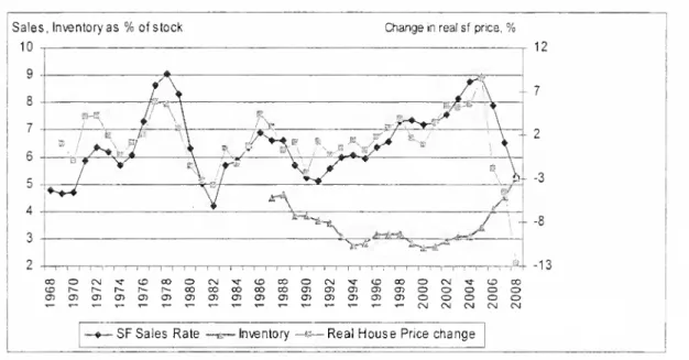
I. Introduction.

As shown

in Figure 1 below, there is a strongpositive correlation

between

housingsales (expressed as a percent ofall

owner

households)and the

movement

in

housingprices

(R

=.66).

On

the surfacethe relationship looksto be closeto

contemporaneous. There isalso a

somewhat

less obviousnegative relationship between

pricesandthe shorter serieson the inventory ofunits for sale

(R

=.51),

A

number

of authorshaveoffered explanations forthese relationships, in particular that

between

prices

and sales.

Figure 1:

US

Housing

Sales,Prices, Inventory

Sales, Inventoryas

%

ofstock 10

Changeinreal stprice,

%

~+^-Z<

^**=N^

12 13

ooorsj-^-cocoocMTrcoooocMTrtocoorM-^-cDco

tor^-r-r^r^r^cococococoa^oa^aicDooooo

T—

^.—

T-T-T-T-r-.—

-^-.—

T-T-T—

T-T-CMCMCMCMCN

SF

Sales Rate Inventory —a

—

RealHousePricechange

On

the one hand, there isa

growing

literature of

models

describing

home

owner

'"churn*" inthe presenceofsearch frictions

[Wheaton

(1990),

Berkovec

and

Goodman

(1996),

Lundberg

and Skedinger (1999)]. In these models, buyers

become

sellers-there

are no entrantsorexits

from

the market. In such a situation ifparticipantspay higher prices, they alsoreceive

more

upon

sale. It is thetransaction costof

owning

2

homes

(duringthe

moving

period) that actually determines price levels.

The

greater transaction costs

accompanying

high pricescan

make

trading expensive

enough

to erase the original gainsfrom moving. In this environment Nash-bargained prices

move

almost inverselyto

salesduration

-

equaltothe vacant inventory divided

by

the sales flow. Inthese models, both the inventoryand sales churn areexogenous. Following Pissarides (2000) ifthe

matching

rate is

exogenous

or alternatively ofspecific form, greatersaleschurn will shorten duration and lead to higherprices. Similarly greatervacancy (inventory) raises sale duration and causes lower prices.

There alsoare aseries of papers

which

proposethat negative changes in prices will subsequently generate lower salesvolumes. Thisagain is apositive relationship

between

the

two

variables, butwith oppositecausality.

The

first ofthese is

by

Stein (1995) followed

by

Lamont

and Stein (1999) and then

Chan

(2001). In these models,

liquidity constrained

owners

areagain

moving

from one house to another(''churn") and

must

make

a

down

payment

in orderto purchasehousing.

When

pricesdecline

consumer

equity does likewise and fewerhouseholds havethe remaining

down

payment

necessary

to

make

a lateral

move.

As

pricesrise, equityrecovers and so does market liquidity.

Relying instead on behavior economics,

Genesove

and

Mayer

(2001) andthen Englehardt (2003)

show

empiricallythat sellers

who

would

loose

some

equity

upon

sale sethigher reservationsthan those

who

would

not.

With

higherreservations, the market as a

whole

should see lowersales if

more

and

more

sellersexperience loss aversion asprices

continue todrop.

Inthis paper

we

tryto unravel the relationship

between

housingprices and

housing sales, and in addition, the inventory of housingunits for sale.

We

accomplish the following:

1). First,

we

carefully

examine

gross housing flows in the

AHS

forthe 1 1 years in

which

thesurvey is conducted and findthere are

more

purchases of

homes

by rentersor

new

households than thereare by existing owners.

Hence

the focuson

own-to-own

trades doesnot characterizethe majorityofhousing sales transactions.

2).

We

also

examine which

flows add tothe inventory offor-sale units (called

LISTS)

and

which

subtract (called

SALES).

'Own-to-own moves,

for

example do

both.

We

show

with a simple

model

oftenure choice flowsthathigherpricesshould generate

more

LISTS,

lower

SALES,

and hence a larger inventory.

When

prices are low, the reversehappens.

3). This leads us to hypothesize a veryspecific form ofjoint causality

between

salesand prices.

Own-to-own

churngenerates a positive schedulebetween sales and

prices as suggested by frictional markettheory. At the

same

time, inter-tenure transitions should lead toa negative schedule. In equilibrium, the overall housing market should rest

atthe intersection ofthese

two

schedules.

4).

To

testthese ideas

we

firstassemble a

US

panel data baseof33

MSA

from 1999-2008.

The

shortnessofthepanel is due to limited data on the for-saleinventory.

An

estimated panel

VAR

model

perfectly confirms ourhypothesized relationships. Sales positively drive subsequent priceswhile pricesnegatively drive subsequent sales andalso positively increasethe inventory.

5).

We

also assemblea longer panel of101

MSA

from 1982 to

2006

onjust sales

and prices.

Using

a

wide

range of

model

specificationsandtests ofrobustness

we

find again thatsalespositively"Granger cause" subsequent housing price

movements,

while

prices negatively"'Grangercause" subsequent housingsales.

These

jointrelationshipsare exactlyas our

model

suggests

when

owner

churn is

combined

with inter-tenure

moves.

Our

paper is organized as follows.In section II

we

setup an accounting

framework

for

more

completely describing gross housing flows fromthe 2001

AHS.

This involves

some

careful assumptionsto adequately

document

the magnitude ofall the

intertenure flows relative towithin tenure churn and to householdcreation/dissolution. In

Section III,

we

develop asimple stylized

model

ofthe inter tenureflowsto illustrate

how

theycan generate a negativerelationship

between

pricesand salesand a positive relationship

between

prices and inventory.

We

present ourhypothesized pair of

relationships

between

pricesand thesales/inventory ratio. In section

IV

we

testthese ideas with a shortpanel data base (33

MSA)

that coversthe inventoryaswell as prices

and sales. In sections

V

through VII

we

present an analysis ofa longer panel dataset

between

just salesandprices across 101

MSA

coveringthe yearsfrom 1982-2006.

Here

again

we

find conclusive evidencethat salespositively"Granger cause" prices and that prices negatively"Granger cause" sales.

Our

analysis is robustto

many

alternative specificationsand subsample tests.

We

conclude with

some

thoughts about historic

II.

US

Gross

Housing

Flows: Sales, Lists,

and

the Inventor}'.

Much

ofthe theoretical literature on sales and prices investigates

how

existing

homeowners

behaveastheytry and sell theircurrent

home

to purchasea

new

one. This flow is

most

often referred to as "churn".

To

investigate

how

important arole "churn" plays in the ownershipmarket,

we

closely

examine

the 2001

American Housing

Survey.

In "Table 10"ofthe Survey, respondentsare asked aboutthe tenureofthe residencethey previously lived in

-

forthosethat

moved

during the lastyear.

The

total

number

of

moves

in this question isthe

same

asthetotal in "Table 11"

-

asking abouttheprevious

statusofthecurrent head (therespondent). In "Table 1

1"

itturns out that

25%

ofcurrent

renters

moved

from a residence situation in

which

they

were

not the head (leaving

home,

divorce, etc.).

The

fraction is a smaller

12%

forowners.

What

is missing is thejoint distribution

between

moving

by the head and

becoming

a head.

The

AHS

is notstrictly

able to identify

how many

current

owners

moved

eithera)

from

anotherunit they

owned

b)anotherunitthey rented orc) purchaseda house asthey

became

a

new

ordifferent

household.

To

generate the full setofflows,

we

use information in"Table 11" about

whether

the previous

home

was

headed bythe currenthead, a relative oracquaintance.

We

assume

that all current

owner-movers

who

were

also

newly

created households -

were

counted in "Table 10" as beingpartofaprevious

owner

household. For renters,

we

assume

that all renter-moversthat

were

also

newly

created households

were

counted in

"Table 10"inproportionto renter-ownerhouseholds inthe full sample. Finally,

we

use the

Census

figures thatyear forthe netincrease in each type of household, and

from

that togetherwith the dataon

moves

we

are able to identify household "exits" bytenure.

Gross household exitsoccur mainly through deaths, institutionalization(such as to a nursing home), or marriage.

Focusingonjustthe

owned

housingmarket,the

AHS

alsoallows usto account

for virtually all oftheevents thatadd units to the inventoryof houses for sale (herein called

LISTS)

and all ofthose transactionsthat

remove

units fromthe inventory (herein called

SALES).

Thereare

two

exceptions.

The

first isthe netdelivery of

new

housing

market. Since

we

have nodirect count ofdemolitions'

we

use thatfigure also as net

and

it is counted asadditional

LISTS.

The

second isthe net purchases of2ndhomes,

which

must

be counted as additional

SALES,

butabout

which

there is simply little data". In theory.

LISTS

-

SALES

should equalthechange in the inventoryofunits forsale.

These

relationships are depicted in Figure 2and can be

summarized

with the identities

below

(2001

AHS

values are included).

SALES

=

Own-to-Own

+ Rent-to-Own

+

New

Owner

[+ 2 nd

homes]

=

5.281.000

LISTS

=

Own-to-Own +

Own-to-Rent

+ Owner

Exits

+

New

homes =

5,179.000 Inventory

Change

=

LISTS -

SALES

Net

Owner

Change =

New

Owners

-

Owner

Exits

+

Rent-to-Own

-

Own-to-Rent

Net

Renter

Change =

New

Renters

-

Renter Exits

+

Own-to-Rent

-

Rent-to-Own

(1)

The

only othercomparabledata is from theNational Association ofRealtors

(NAR).

and itreports that in2001 the inventory ofunits for sale

was

nearly stable.

The

NAR

however

reportsaslightly higher level ofsales at 5.335.000 existing units. This small discrepancy could beexplained by repeat

moves

withina

same

year since the

AHS

asksonlyaboutthe

most

recent

move.

Itcould also represent 2nd

home

sales

which

again are not partofthe

AHS

move

data.

What

is

most

interesting to us is that almost

60%

of

SALES

involve a buyer

who

is nottransferringownership laterally from one

owned

houseto another.

So

called

"churn"is actually a minorityofsalestransactions.

The

variousflows

between

tenure categoriesalso arethe

more

critical determinant ofchange-in-inventory since"churn"

salesleave the inventory unaffected. .

Thegrowth in stockbetween 1980-1990-2000 Censusescloselymatchessummedcompletionssuggesting

negligibledemolitionsoverthosedecades. The samecalculation between 1960 and 1970howeversuggests

removal of3 millionunits.

2

Netsecondhomepurchasesmight beestimatedfromtheproductof: theshareoftotal grosshome

purchasesthat aresecondhomes(reported by LoanPerformanceas 15.0%) andtheshare ofnew homes in total homepurchases(Census,25%). Thiswouldyield 3-4%oftotaltransactionsorabout200,000units.

Therearenodirectcountsoftheannualchange in2" homestocks.

The

AHS

isarepeatsample of housingunitsand excludesmovesintonewhouses.Thuswecompare its

Figure2:

US

Housing

Gross Flows

(2001)

>nd

Net

2

Home

Purchases

(SALES)

(1)

New

Owner

households

=

564,000

(SALES)

Renterto

Owner

=

2,468.000

(SALES)

(1)

New

Renter households

=

2.445,000

Owner

to

Owner

=

2,249.000

(LISTS

&

SALES)

Owners =

72,593,000

Net

Increase

=

1,343,000 Renters

=

34,417,000

Net

Increase

=

-53,000 Renterto Renter

=

6,497.000 (2)

Owner

Exits

=

359,000

(LISTS)

Owner

to Renter

=

,330,000

(LISTS)

Net

New

Homes

=

1.242,000.

(LISTS)

(2) RenterExits

=

1,360,000

In Figure 2.

most

inter-tenure

SALES

would

seem

to be eventsthatone might expectto be negatively sensitive tohousing prices.

When

prices are high presumably

new

created

owner

household formation is discouraged orat leastdeflected into

new

renter

household formation. Likewise

moves

which

involvechanges intenure from renting to

owning

also should be negatively sensitive tohouse prices.

Both

result becausehigher pricessimply

make

owning

a house lessaffordable.

At

thistime

we

are agnostic about

how

net 2nd

home

salesare related to prices.

On

theotherside ofFigure 2,

many

ofthe events generating

LISTS

should be at

least

somewhat

positively sensitive to price.

New

deliveries certainlytryto occur

when

to "cash out",

consume

equity orvoluntarilychoose to switchto renting. Atthis time

we

are still seeking a direct data source

which

investigates in

more

detail

what

events tend to generate the own-to-rentmoves.

Thus

theflows inand outof

homeownership

inFigure 2 suggestthat

when

prices are high sales are likely to decrease lists increaseandthe

inventory grow.

The

AHS

hasbeen conducted only semi-annually until recently and alsohas used consistentdefinitions of

moving

only since 1985. In

Appendix

III

we

calculate the flows

foreachofthe 11

AHS

surveys between 1985 and 2007.

The

flows are remarkably

stable, although there exists

some

yearto yearvariations. In all years,

own-to-own

moves

("chuirT) are less thanthe

sum

of

new

owners

plus rent-to-ownmoves. Sincethe2001 survey, the

AHS

calculated values for

LIST-SALES

have increased significantly. This is

consistent withthe

growing

national for-sale inventory reported in the

NAR

dataover

this period.

III.

A

stylized

model

of inter-tenureflows.

Here

we

assume

that thetotal

number

of households

T

is fixed with

H

<

T

being

home

owners.

Those

not

owning

rent at

some

fixed (exogenous) rent

-

hence

we

largely ignore the rental market.

The

total stockofunitsavailable for ownership U(p) is

assumed

to

depend

positively on price (longrun supply) and with fixed rents

we

ignore rental supply. In this situation the inventoryofunits for sale is the difference between the

owner

stockand

owner

households: I

=

U(p)

-

H.

Households

flow outof ownershipat

some

constant ratea

which

could represent

unemployment,

foreclosure,or other

economic

shock. Rental households purchase units out ofthe

owner

stock

(become

owners)at

some

rate s(p)

which

we

presume

depends negativelyon price.

High

prices (relative to the fixed rent)

make

ownership less

appealing, but in general renterswishto

become

owners

becauseof

some

assumed

advantage(atax subsidy forexample).

-

hencethe purchaserate isalways positive.

The

equations

below

summarize

both flows (timederivatives) andsteady state

values (denoted with *). In Equation (2) the stable

homeownership

ratedepends

negativelyon prices and the constant

economic

shock rate.

When

pricesgenerate a sales rate equal to the

economic

shockrate,

homeownership

is

50%.

Equation (3) cleanly

divides up the inventory

change

intothe

same

two

categories

from

our

more

detailedflow diagram:

LISTS-SALES.

Here

LISTS

are stockchange

(new

construction) plus

own-to-rent flows

(economic

shocks) while

SALES

are rent-to-own flows.

The

equilibrium level

of

SALES

is in (5),and the equilibrium inventory in (4).

The

latter

must

beconstrained positive.

dH/dt

=

s(p)[T-H]-aH,

H'

=

S("

P)T

(2)

a

+

s(p) dlIdt

=

dU

Idt

-

dH

Idt

= [dU

Idt

+

aH]-

s(p)[T

- H],

(3 )

l'=U(p)-H'

=

<*U(P)

+ s(P)U(P)-sT>o

₍₄₎

a

+

s{p)

.

as(p)T

s(p)[T-H

]

=

—

(5)

a

+

s{p)

In (6)

we

derive comparative statics

which

show

thatas prices increase,the steady

state valueofthe inventory

grows

and thesteady state level of

SALES

decreases

-

as

hypothesized aboutthe flows

which

were diagramed

in Figure 2.

dl' I

dp

= dU/dp-dH'

/dp

=

dU/dp-

P

[\

—

^7

>0

(6)

a

+

s a

+

s

d

(s(

_P

)[T-H'])/dp

=

£™^[l-^_]

<

a

+

s

a

+

s

Again,the conclusions

above

follow from theassumptionsthat long run stock is positively related toprice and the salesrate is negative relatedto price.

Thus

thissimple

model

ofinter-tenure flows establishes a negative relationship

between

housingprices

and Sales/Inventoryratios. Alternatively, there should bea positive relationship

between

pricesand duration.

With

this

new

schedule

between

pricesand duration

we

are

now

readytobetter describethe full setofrelationships in the

owner

market

between

sales, pricesand the inventor)'.

We

combine

this

new

schedule with a positive schedule

between

prices and the Sale/Inventory ratio

-

created fromthe various

models

of

own-to-own

decisions. In

these latter

models

itis sales that are determining prices, while with the

model

in (2)-(5)

above

it is prices that aredeterminingsales.

At

a

more

complete equilibrium (in the

ownership market) sales, pricesand the inventory all rest atthe intersection ofthe

two

schedules

shown

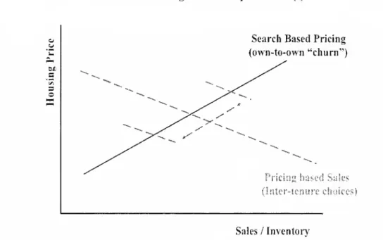
in Figure3. Figure 3 presents a

more

completepicture ofthe housing market thanthe

models

ofStein,

Wheaton,

or

Berkovec

and

Goodman

-

since itaccounts

forthevery large role ofinter-tenure mobility aswell as for

owner

churn.

FIGURE

3:

Housing

Market

Equilibrium(s)

Search BasedPricing (own-to-own "churn")

WO

Pricingbased Sales (Inter-tenure choices)

Sales/Inventory

The

out-of-equilibrium

dynamics

ofthis

model

are alsoappealing and

seem

in

linewith

economic

intuitionas well. Considera permanentincrease in

economic

shocks

(a).

Using

(2)- (5),

owner

householdsdecline, andthe inventory increases. Sales

however

also increaseand sothe impact on duration is technically ambiguous. Within a

wide

range ofreasonable parametervalues however,

we

can

show

that the sale/inventoryratio

declineswith greatera

-

the netshift in the price-to-sales schedule is therefore inward.

The

new

equilibrium then results in lowerprices with a lowersales/inventory ratio as well (a higherduration). If

we

shiftthe s(p) scheduleup (e.g. a greater tax subsidy)the

number

of

owners

increases, the inventory drops, and sales increase. This leadsto an

4

unambiguous

rightward shift in the price-to-salesschedule with a corresponding rise in

equilibrium Sales/Inventory (drop in duration). Pricesof course rise as well.

The

next task isto see if

we

canempirically identifythe relationships in Figure 3.

Forthis,

we

examine

two

several panel databases with different degreesofrichness.

The

first data base isshorterand covers only 33

MSA.

Its advantage isthat it includes data

on

the inventory for sale by market

-

a series

which

the

NAR

has collected only recently.

The

second database is

much

longer, covers 101

MSA,

but includes only information

on

sales and prices.

IV.

A

Short Panel

Analysis of

Metropolitan

Sales, Prices

and

Inventory.

Carefully constructed series on house prices areavailable from the late 1970sor early 1980s and fora

wide

rangeofmetropolitan areas.

The

pricedata

we

use isthe deflated

OFHEO

repeat sales series [Baily,

Muth,

Nourse

(1963)].This data series has recently been questioned fornot factoring out

home

improvements

ormaintenance and

fornot factoring in depreciation and obsolescence [Case,Pollakowski,

Wachter

(1991), Harding. Rosenthal, Sirmans (2007)]. Thatsaid

we

are leftwith

what

isavailable, and

the

OFHEO

index is the

most

consistent series available for

most

US

markets overa long

timeperiod.

The

only alternative is

CSW/FISERV,

and it is available forfar fewer metropolitan areas that in turn aredisproportionately concentrated in the south and west.

In termsofsales,the only consistent source isthatprovided

by

theNational Association ofRealtors

(NAR).

The

NAR

data is forsingle family unitsonly (it excludes

condominium

sales atthe

MSA

level), butis availableforeach

MSA

over a period

from

1980to the present.

The

more

limitingdata series is thaton the inventory of housing

units forsale.

Here

the

NAR

distributes

MSA

data only from 1999 orlater.

We

have been

able toputtogetherall three series since 1999 for33

MSA,

and Figures4 through 6 depictthe 33 series foreach variable.

The

patterns arequitediscernable and in

Appendix

I

we

present

summary

statisticsforeach market.

In Figure 4

we

clearly see all house prices risingand thenfalling since 1999.

The

sample almost evenly divides

between

market

where

this

movement

is very

pronounced

and those with onlythe slightestofchanges. Interms ofthe inventory, Figure 5

shows

thatover the firsthalfofthe samplethe inventory

was

roughly constant. After

2004

it

rises and falls in a pattern again similarto prices. Boththe Pricesand Inventoryare

raw

series andexhibit little seasonality.

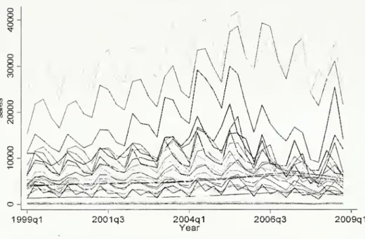
As

forsales, in Figure 6

we

see a littlebit ofthe

same

"hump

shaped"pattern, but it

seems

weaker.

What

is

more

problematic with the sales data is thestrong pattern ofseasonality in each series

-

seasonalitythatvaries by specific

market in

many

cases.

Figure4:

Quarterly Real

House

Prices (33

MSA),

1999-2008

o

in

n

o

o

o

OJ D.

E

o

o

O

o

o

-1999q1

2001q3

2004q1 Year 2006q3 2009q1

Figure5:

Quarterly

For-SaleInventory (33

MSA),

1999-2008

o

o

o

o

o

m

o

o

o

o

o

\r

o

o

o

o

o

Q) CO

o

o

o

o

o

o

o

o

1999q1 2001q3 2004q1 Year 2006q3 2009q1 13

Figure

6:

Quarterly

House

Sales (33

MSA),

1999-2008

o

9

c

c

c

o

n

8g

o

o

CM

1

o

8

o

1999q1 2001q3 2004q1 Year 2006q3 2009q1

These

observations suggestthata panel

VAR

is an appropriate instrumenttotest

the relationships

between

prices, sales and inventory. In the

VAR

we

will have each variable depending on lagged values ofitselfand theothervariables. Ifthe panel is of order one,

we

also can use each coefficient asaneffectivetestof

"Granger

causality".

Before turningto such amodel, however,

we

needto

examine

each seriesto see ifthey are stationary. Thereare

two

tests available foruse with panel data and in each, the null hypothesis is that

sum

oraverageofallthe individual series have unit rootsand are

non

stationary. In Levin-Lin (LL, 1993) the null hasno constant(ordrift)while in

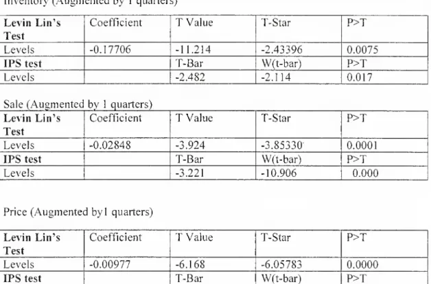
Im-Persaran-Shin (IPS, 2002) the null includes a constantto allow fordrift. In Table 1

we

reportthe resultsofthis testfor housingprices, sales and inventory

-

in levels.

With

the possible exception ofprices,

where

we

can be confident only atthe

7%

level, the non-stationary null is rejected and

we

should be on solid grounds undertaking our proposed

VAR.

Table

1: Stationary tests,Short Panel

Inventory'

(Augmented

by 1 quarters)

Levin

Lin's

Test

Coefficient

T

Value T-Star

P>T

Levels -0.17706 -11.214 -2.43396 0.0075

IPS

test

T-Bar

W(t-bar)

P>T

Levels -2.482 -2.114 0.017

Sale

(Augmentec

by 1 quarters)

Levin

Lin's

Test

Coefficient

T

Value T-Star

P>T

Levels -0.02848 -3.924 -3.85330 0.0001

IPS

test

T-Bar

W(t-bar)

P>T

Levels -3.221 -10.906 0.000

Price

(Augmented

byl quarters)

Levin

Lin's Test

Coefficient

T

Value T-Star

P>T

Levels -0.00977 -6.168 -6.05783 0.0000

IPS

test

T-Bar

W(t-bar)

P>T

Levels -1.750 -1.477 0.070

In panel

VAR

models

with individual heterogeneitythere exists a specification issue: the errorterm can becorrelatedwith the lagged dependent variables [Nickell, (1981)].

OLS

estimation can yield coefficients that areboth biased and also that arenot consistent in the

number

ofcross-section observations. Consistency occursonly in the

number

of time series observations.

Thus

estimatesand anytests on theparameters of

interest

may

notbereliable.

These

problems might notbe serious inourcase since

we

have 32 quarterlytime series observations(morethan

many

panel models).

To

be on the

safe side, however,

we

also estimated the equations following an estimation strategy by

Holtz-Eakin et al.

As

discussed in

Appendix

II, this

amounts

to using 2-period lagged values ofsales andprices as instruments with

GLS

estimation.

A

final concern with our

VAR

isthe handlingofseasonality.

Here

we

propose 2

adjustments. In Tables 2and 3,

we

report results using quarterly seasonal effects

interacted withthecross section fixed effects. This effectivelyallows each

MSA

to have its

own

setofseasonal influences.

Our

second approach isto change all ofthe lags inthe

VAR

to4-periods ratherthan one. In effect

we

areasking

how

ourvector ofvariables

relates to thevector lagged a year previousratherthan a quarter ago.

The

year-over-year

VAR

results are presented in Table 4.

5

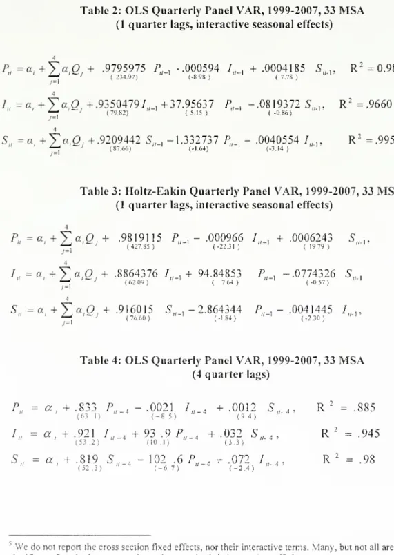
Table

2:

OLS

Quarterly Panel

VAR,

1999-2007,

33

MSA

(1

quarter

lags, interactive seasonal effects)

P=a

+YaO,+

.9795975

P

u . -.000594 /„ ,

+.0004185

S,

n

,

R

2

=0.9889

" '

4f

'*-> (234.97) ""' (-8,98) ""' (7,78) ""' 4 /

=

a,

+Y

a,O,

+.93504797,

.

+37.95637

P..

-.0819372

5,,.,

R

2

=.9660

" '

^

'-' (79.82) ""' (5.15) ""' (-0.86) ""'' 4

S

=a+Ya,0,

+.9209442

S

_u .

-1.332737

P. ,

-

.0040554 /„..

R

2

=.9950

(87.66) (-164) (-3.14)

Table

3:

Holtz-Eakin Quarterly Panel

VAR,

1999-2007, 33

MSA

(1

quarter

lags, interactive seasonal effects)

p

'

=

a

,

+

Y

a,0,+

.9819115 P..

.-

.000966 I...

+.0006243

S.

n

, " '

j^

'~> (427.85) ""' (-22.31) ""' (1979) ""' 4 /

=

a

.

+

Y

a,Q,

+

.8864376 /„ ,

+

94.84853 P„ ,

-

.0774326 S„ , " '

^

' («09) """' ( 764) "-' (-0.57) ""' 4 S.

=

a,.

+Ya,.0,T

.916015 5„

,-

2.864344

P,

.-

.0041445 /, ,, '

^

J (76.60) "-l (-184) ""' (-2.30) ""'

Table

4:

OLS

Quarterly

Panel

VAR,

1999-2007,

33

MSA

(4

quarter

lags)

P„

=

a,

+

.833

P„

₄

-

.0021 /„ ₄

+

.0012

5,

4,

R

-

=

_.885 (63 1) "-4 (-S 5) ""4 (9 4) "" 4 ' /„

= a, +

.921 /„_<

+93

.9/>„_₄

+

-032 5„.4>

R

2

=

.945 (53 .2) (10.1) (3 3)

S„

= a,

+.819

S„_

₄

-102

.6

P„_

4

-.072

7„.4 ,

R

2

=

.98 (52 .3) (-67) (-2.4) 5

We

donot report the cross section fixed effects,northeirinteractiveterms. Many, butnotallare

significant.Standarderrorsareshownin parenthesisbeloweach coefficient.

In

examining

Tables2-4,

we

find that ourthree hypotheses are validated in every case. First,the inventory negatively impactsprice while sales hasa positive effect.

Interestingly thecoefficienton inventory is alwaysslightly largerthansales. Ina log

model

ifthe ratio(duration)

were

all thatmattered the coefficients

would

be identical in

magnitude. In this linear

model

theyare close

enough

to suggesta similarconclusion. Secondly, the inventory respondsquite significantly (and positively) to prices. Thirdly, prices negatively impact subsequent sales. All ofthese effects are statistically significant, but the price impact on Sales

shows up

more

strongly inthe 4-quarter lagmodel. In the

1-quarter

model

itis atthe thresholdofsignificance. In all respects, the results fully support equations (2)-(5) and the pairofrelationships in Figure 3. Duration negatively

"Granger

causes" subsequentprices to decline. Pricethen positively

"Granger

causes" the

inventoryto grow, and likewise for sales to decline.

The

first

VAR

equation validates the

upward

schedule in Figure3 whilethe secondand third

combine

to yield the

downward

schedule.

In

comparing

the different

models

we

note that the Holtz-Eakin estimation does increasethe coefficients abitand reduce standard errors

-

relative to the

OLS

results.

We

did notundertake Holtz-Eakin estimation for our 4-quarter lag model.

The

OLS

4-quarter results areexpected!}' different. Inventoryand sales, forexample, have an impacton

prices4 periods hencethat is roughly4 timestheir impact inthe 1_-quarter model.

Similarly, prices impactsales 4 quarters hencewith

much

greater impactthan fromjust 1

quarterback.

V.

A

long-PanelofMetropolitan Sales

and

Prices.

It is possible totestthe just the relationshipbetween prices and salesovera

much

longertime horizon

-

if

we

ignore theinventory.6 Forthis

we

assemblea larger panel data base covering 101

MSA

and spanning theyears 1982 through 2006. This panel

was

6

There have beenafewrecentattemptstestthe relationshipbetweenmovementsinsales andprices. Leung, Lau, andLeong(2002) undertakeatimeseriesanalysisofHong KongHousing and concludethat

strongerGrangerCausalityisfoundforsalesdrivingprices ratherthan pricesdrivingsales. Andrewand

Meen(2003)examinea

UK

Macrotimeseriesusinga

VAR

model andconcludethattransactions respond toshocksmorequickly thanprices,butdonot necessarily "GrangerCause"priceresponses. Bothstudies

arehamperedby limited observations.

purposely structured to be annual so asto avoid the seasonalityofthe shorter panel,while still maintaining plentiful time-based degrees of freedom.

Over

this longer period,

many

metropolitan areas almostdoubled theirhousing stock so

we

decided to standardizethe salesdata to eliminate

some

ofthe trend.

Raw

sales

were

compared

with yearly

Census

estimates ofthe

number

oftotal households in

those markets. Dividing singlefamily sales

by

total households

we

getan estimated sales rate for each market in each period.

Using

sales rates also eliminated

much

ofthecross section variation inthe

raw

number

ofsales. In a similar

manner

we

setthereal price level in each marketto 100 in the baseyear.

These

re-scalingofthe datawill help

make

thecross section fixed effects smaller in the estimated

VAR

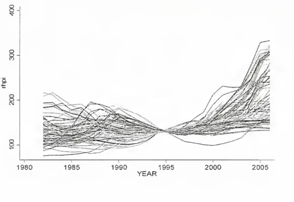
models.

In Figures 7and 8

we

illustratethe constant dollar

OFHEO

price seriesalong with the yearly

NAR

sales rate data, forall 101 of ourmarkets.

Over

this time frame, the priceseries vary widelyacross markets, with

some

areas experiencing long term

although episodic increases (e.g. San Francisco)while othersare almosttotally constant

(e.g. Dallas).

As

forthe salesrates, virtually everymarkethas aslow gradual trend in

salesrates, with the

sample

average increasing from

3%

to 5.6

%.

InappendixIII

we

presentthe

summary

statistics for each market'sprice and sales rate series.

The

data in Figure 4through 6 forthe shortpanel

showed

no obvioustrends;'

prices, sales and the inventory generallyriseand then fall.

The

longerterm series in

Figures 7 and 8

may

have

more

persistenttrends and so again

we

need to test for

whether

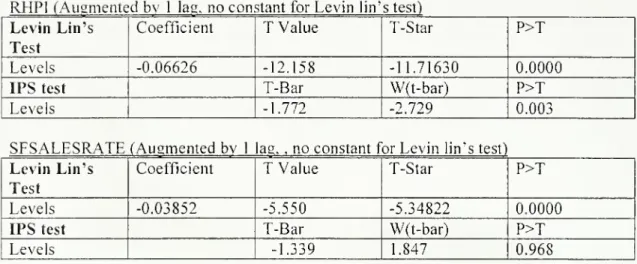
theseries are stationary. InTable 5

we

reporttheresults ofboth Levin-Lin and IPStests forboth housing priceand sale rate levels.

With

bothtests the null for house prices is rejected athighconfidence levels, but

withthe IPS testthe null hypothesis forthe sales rate is quite likely to hold.

Given

the steady trends seen in Figure 8, this of course

seems

reasonable.

To

be onthe safe side,

then

we

estimateour long term sales-price

VAR

in differences aswell as levels.

Figure7:

Annual House

Prices (101

MSA),

1982-2006

o

o

CO a.

o

o

1980 1985 1990 1995

YEAR

2000

2005

Figure8:

Annual

Sales

Rate

(101

MSA),

1982-2006

CD a CO Lf) 1980 1985 1990 1995

YEAR

2000

2005

l"

TABLE

5: Stationary tests,

Long

Panel

RHPI

(Augmented bv

1 lag, no constant forLevin lin's test)

Levin

Lin's Test

Coefficient

T

Value

T-Star

P>T

Levels -0.06626 -12.158 -11.71630 0.0000

IPS

test

T-Bar

W(t-bar)

P>T

Levels -1.772 -2.729 0.003

SFSALESRATE

(Augmented

bv

1 ag. .

no

constantfor Levin lin's test)

Levin

Lin's Test

Coefficient

T

Value

T-Star

P>T

Levels -0.03852 -5.550 -5.34822 0.0000

IPS

test

T-Bar

W(t-bar)

P>T

Levels -1.339 1.847 0.968

Since

economies change

more

in the longer term,

we

decided to include several conditioning variables.

The

conditioning variables

we

choose are market specific

employment,

and thenational

mortgage

rate.

The

resulting 2-variable

VAR

in levels is

shown

in(7), while in(8) the

companion model

ispresented in first differences.

P,j

_{=ao+«i p}

/.,-i

+«aV,

+

/7'^//

+

3

+*,.,

Su

=7o

+

r,Vi

+/2

P

U-\+^

X

U +

7_l

+£

u

AP,,

=a +a

i

AP

IJ_l

+a

2

AS

_IJ_l

+/3'AX

_IJ

+5,

+£,, ^,.«

=7o +

/i

A

V>

+y

2&P,.l_i

+A

,

AX,

J +?],

+£

(7) (8)

We

estimateeach

model

using both

OLS

andalso applying the previously discussed estimation strategy

by

Holtz-Eakin etal.

From

either estimates,

we

conduct a

"Granger"

causalitytest. Since

we

are onlytesting for a single restriction, the t statistic is the square root ofthe

F

statistic that

would

be used to testthehypothesis in the presence ofa longer lag structure (Greene,2003). Hence,

we

can simply use a ttest (appliedto

7

In (6)the fixedeffects arecross-section trendsratherthan cross sectionlevels asin(5)

thea, and

_y

₂)as thecheck ofwhether changes in sales"Granger cause" changes in price and/orwhetherprices

"Granger

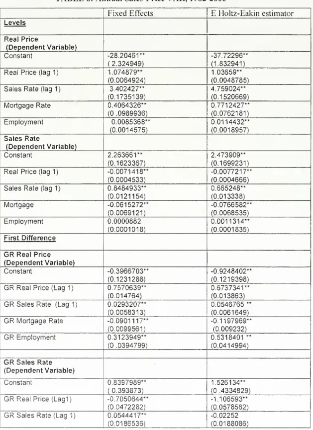
cause" sales.

In table 6

we

report the results ofequations(7) and(8) in each setofrows.

The

first

column

uses

OLS

estimation, thesecond the

Random

Effects

IV

estimates

from

Holtz-Eakinet al. Interestingly, the

two

estimation techniquesyield quite similar coefficients

-

asmight be expected with a larger

number

oftimeseries observationsand datarescaling to reduce the cross sectioneffects.The first setofequations is in levels,

while the second setof

rows

reportsthe resultsusing differences. In all Tables, variable

names

are selfevidentand variable differences are indicatedwith the prefix

GR.

Standard

errors are reported in parenthesis.

Among

the levels equations,

we

firstnotice

some

anomalies.

The

mortgage

interest rate inthe price levels equation is always ofthe

wrong

sign, andthe

employment

coefficient inthe

OLS

sales rate equation is insignificant (despitealmost

2500

observations).

A

more

troublesomeresult isthat the price levelsequation has excess

"momentum"

-

lagged priceshave acoefficientgreaterthan one.

Hence

prices (levels)

can

grow

on their

own

without necessitating any increases in fundamentals, orsales.

We

suspectthatthese

two

anomaliesare likely the resultofthe non-stationary feature toboth the price andsales series

when

measured

in levels.

When we move

tothe results of estimating theequations in differences all ofthese issues disappear.

The

lagged price coefficients are lessthan one so the price equations are stable in the 2n degree, and the signsofall coefficients are both correct

-

and highly significant.

As

tothe question ofcausality, in everyprice orprice growth equation, lagged sales orgrowth in sales is always significantly positive.Furthermore in every salesrate or growth in sales rateequation, lagged prices (or itsgrowth) arealso alwayssignificant.

There is clearevidence ofjoint causality,

and

the effect

of

laggedprices

on

salesis

always

of a

negativesign. Holding lagged sales (and conditioning variables)constant, a

yearafterthere is an increase in prices

-

salesfall. Thisisthe opposite ofthatpredicted

by

theories ofloss aversion or liquidity constraints, butfully consistentwiththe role

playedby tenurechoices in Figure2 and our simple

model

ofthese flows.

TABLE

6:

Annual

Sales-Price

VAR,

1982-2006

Fixed Effects

E

Holtz-Eakin estimator Levels Real Price (DependentVariable) Constant -28.20461** ( 2.324949) -37.72296** (1.832941) Real Price (lag 1) 1.074879**

(0.0064924)

1.03659** (0.0048785) Sales Rate (lag 1) 3.402427"

(0.1735139) 4.759024** (0.1520669) MortgageRate 0.4064326** (0 .0989936) 0.7712427** (0.0762181) Employment 0.0085368** (0.0014575) 0.0114432** (0.0018957) Sales Rate (DependentVariable) Constant 2.263661** (0.1623367) 2.473909** (0.1699231) Real Price (lag 1) -0.0071418**

(0.0004533)

-0.0077217** (0.0004666) Sales Rate (lag 1) 0.8484933**

(0.0121154) 0.665248** (0.013338) Mortgage -0.0615272** (0.0069121) -0.0766582** (0.0068535)

Employment

0.0000882 (0.0001018) 0.0011314** (0.0001835) First Difference

GR

Real Price (DependentVariable) Constant -0.3966703** (0.1231288) -0.9248402** (0.1219398)

GR

Real Price (Lag 1) 0.7570639**

(0.014764)

0.6737341** (0.013863)

GR

Sales Rate (Lag 1) 0.0293207**

(0.0058313) 0.0546765 ** (0.0061649)

GR

MortgageRate -0.0901117** (0.0099561) -0.1197969** (0.009232)

GR

Employment

0.3123949** (0 .0394799) 0.5318401 ** (0.0414994)

GR

Sales Rate (DependentVariable) Constant 0.8397989** ( 0.393873) 1.526134** (0 .4334829)

GR

Real Price(Lag1) -0.7050644**

(0.0472282)

-1.106593** (0.0578562)

GR

SalesRate (Lag 1) 0.0544417**

(0.0186536)

-0.02252 (0.0188086)

GR

Mortgage Rate -.3251265" (0.0318483) -0.3078643** (0.031781)

GR

Employment 1.134269** (0.126291) 1.391958** (0.1463704) ** _{indicates significanceat}

_5%.

We

have experimented with these

models

using

more

thana single lag, but qualitatively the results are the same. In levels, the priceequation with

two

lags

becomes

dynamically stable in thesensethatthe

sum

ofthe lagged price coefficients is lessthan one.

As

tocausal inference, the

sum

ofthe lagged sales coefficients ispositive, highly significant, and passes the

Granger

F

test. Inthe salesrate equation,the

sum

ofthe

two

lagged sales rates is virtually identical tothe single coefficient

above

andthe lagged price levelsare again significantly negative(in theirsum). Collectively higher lagged prices

"Granger

cause"a reduction in sales.

We

have similarconclusions

when

two

lags are

used in the differences equations, but indifferences, the 2nd lag isalways insignificant.

As

a final test,

we

investigate arelationship between the

growth

in house prices

and the levelofthe salesrate. Inthe search theoretic

models

sales ratesdetermine price

levels,but ifprices are

slow

to adjust,the impactofsales mightbetter

show

up on price

changes. Similarly the theoriesofloss aversionand liquidityconstraints relate price

changesto sales levels.

While

the mixing oflevelsand changes in time seriesanalysis is generally not standard, thiscombination ofvariables is alsothestrong empirical fact

shown

in Figure 1. InTable 7 pricechanges are tested for

Granger

causality againstthe level ofsales (as a rate).

TABLE

7:

Annual

Sales-Price

Mixed

VAR,

1981-2006

Differencesand Levels Fixed Effects

_E

_Holtz-Eakin estimator

GR

Real Price (DependentVariable) Constant -6.698605** (0.3568543) -11.10693** (0.4174099)

GR

Real Price (lag 1) 0.5969905**

(0.015889)

0.4286127** (0.0156827) Sales Rate (lag 1) 1.424051**

(0.0760102) 2.340478** (0.0912454)

GR

Mortgage Rate -0.1230876** (0.009451) -0.1573441** (0.0086482)

GR

Employment 0.4987545** (0.0349922) 0.7781044** (0.0373462) 23

Sales Rate (DependentVariable) Constant -0.0458271" (0.0541373) 0.283191" (0.0642588)

GR

House

Price (lag 1) -0.0328973"

(0.0024105)

-0.0355432" (0.002961) Sales Rate (lag 1) 1.01549"

(0.0115313) 0.9482599" (0.0139037)

GR

Mortgage Rate -0.0156137" (0.0014338) -0.0132519" (0.0013497)

GR

Employment

0.0462483" (0.0053086) 0.7280071" (0.1643153) ** _{indicatessignificance at}

_5%

In terms

of

causality,these results areno different than the

models

estimated either in all levelsorall differences.

One

yearafteran increase in the levelofsales, the

growth

in house prices accelerates. Similarly, one yearafterhouseprice

growth

accelerates the levelof

home

salesfalls. All conditioning variables are significantand correctly signed and lagged dependent variableshave coefficients lessthan one.

VII.

Long

Panel

Tests ofRobustness.

In panel

models

it is alwaysa

good

ideatoprovide

some

additionaltests ofthe robustness ofresults, usually by dividingup eitherthe cross section ortime series

of

the panel intosubsets and

examining

theseresults aswell.

Here

we

perform bothtests. First

we

divide the

MSA

markets into

two

groups: so-called "coastal" citiesthatbordereither ocean, and "interior" citiesthat

do

not. There are31 markets in the former group and

70

in the latter.

The

coastal citiesareoften feltto bethose with strong price trends and possibly different market supply behavior.

These

results are in Table 8.

The

second test is

to dividethe

sample

up

by

year

-

inthis case

we

estimate separate

models

for 1981-1

992

and 1993-2006.

The

year 1992generally

marks

thebottom ofthe housing market

from

the

1990

recession.

These

results are depicted in Table 9.

Both

experiments usejustthe differences

model

that

seems

toprovidethe strongest results

from

the previous section.

TABLE

8:

Geographic

Sub

Panels,

1982-2006

FixedEffects EHoltz-Eakin estimator

Coastal

MSA

Interior

MSA

Coastal

MSA

Interior

MSA

GR

Real Price (Dependent Variable) Constant -0.4766326** (0.272633) -0.3510184 (0.130979) -1.188642** (0.2669406) -0.721773" (0.1290227)

GR

Real Price (Lag1) 0.7340125** (0.0271992) .77654** (0.0173987) 0.6845244** (0.0255055) 0.6926984** (0.0162093)

GR

Sales Rate (Lag 1) 0.0615042** (0.0133799) 0.016732** (0.0061206) 0.089245** (0.0135344) 0.0373314** (0.0064948)

GR

Mortgage Rate -0.0885175** (0.0214447) -0.0908632** (0.0107238) -0.1275495** (0.020204) -0.1119299** (0.0098326)

GR

Employment 0.413934** (0.0864868) 0.2599301** (0.0422536) 0.6823408** (0.0890938) 0.4168953** (0.0438112)

GR

Sales Rate (Dependent Variable) Constant 1.01577** (0 .71945) 0.726351** (0.4706282) 0.9888512** (0.7707496) 1.406108** (0.5151945)

GR

Real Price (Lag1) -0.7510799** (0.0717759) -0.680113** (0.0625164) -0.9596828** (0.0802649) -1.092057** (0.0775659)

GR

Sales Rate (Lag1) -0.0111514 (0.0353082) 0.0786527** (0.0219922) -0.0686389** (0.0362451) .013674 (0.0219432)

GR

Mortgage Rate -0.3092647** (0.0565903) -0.3335691** (0.0385322) -0.3139948** (0057035) -.3112734** (0.0383706)

GR

Employment 1.265646** (0.2282296) 1.097809** (0.1518239) 1.651104** (0.2580107) 1.285375** (0.1738679) Note: a) *- 10 percent si b)

MSAs

denoted c)

MSAs

denoted

gnificance. **- 5 percent significance.

coastal are

MSAs

nearthe East or

West

Coast(see

Appendix

I).

interiorare

MSAs

that arenot located at the East or

West

Coast.

InTable 8, the results of Table 6 holdup remarkably strong

when

the panel is divided by region.

The

coefficientofsales rate (growth)on prices is always significant although so-called "costal"citieshave larger coefficients. In the equationsofprice

(growth) on salesrates,the coefficients are alwayssignificant, and thepoint estimates are very similar as well.

The

negativeeffect ofprices on sales rates is completely

identical across the regional division ofthe panel sample. Itshould be pointed outthat all

ofthe instrumentsare correctlysigned and significantas well.

The

conclusion isthe

same

when

thepanel is split into

two

periods (Table 9).

The

coefficients ofinterestare significantand ofsimilar magnitudes acrosstime periods, and

all instruments are significantandcorrectly signed as well.

The

strongnegative impact of

priceson sales clearlyoccurred during

1982-1992

as wellas overthe

more

recentperiod

from

1993-2006.

With

fewer time series observations in each ofthe(sub) panels in

Table9, the Holtz-Eakin estimatesare

now

sometimes

more

differentthan the

OLS

results.

TABLE

9:

Time

Subpanels,

101

MSA

Fixed Effects

E

Holtz-Eakinestimator

1982-1992 1993-2006 1982-1992 1993-2006

GR

Real Price (Dependent Variable) Constant -2.648239** (0.2403419) 0.1098486 (0.1788311) -2.597524** (0.2538611) 0.0280176 (0.1594721)

GR

Real Price

(LaaU

.5533667** (0.0273908) 0.7581002** (0.0202692) 0.7006637** (0.0281998) 0.709152** (0.0212374)

GR

Sales Rate (Lag 1) 0.0204875** (0.0074812) 0.0631485** (0.0114222) 0.0273097** (0.0081297) 0.0373903** (0.0114339)

GR

MortgageRate -0.2309851** (0.0195574) -0.113025** (0.0148469) -0.2164034** (0.0174734) -0.1088119** (0.0120579)

GR

Employment

0.6215331** (0.0644479) 0.3634738** (0.0594376) 0.5073589** (0.0719732) 0.5722806** (0.0629962)

GR

Sales Rate (Dependent Variable) Constant -6.077011** (0.9073653) 3.339319** (0.494379) -4.553209** (1.017364) 4.601864** (0.5978177)

GR

Real Price (Lag1) -0.8804394** (0.1034087) -0.7628642** (0.0560344) -0.9065855** (0.1359358) -0.8880742** (0.0738609)

GR

SalesRate (Lag 1) 0.0053538 (0.0282439) -0.0100386** (0.0315767) 0.0706683 (0.0302102) -0.0313258 (0.035461)

GR

Mortgage Rate -0.5534765** (0.0738353) -0.3843505** (0.0410443) -0.5593403** (0.0731325) -0.2695104** (0.0383087)

GR

Employment

2.564815** (0.2433108) 0.7280071** (0.1643153) 1.88701** (0.293079) 0.5015754** (0.2095683) Note:

a)

Column

labeled under 1982-1992 refer tothe results using observationsthat span those years..

b)

Column

labeled under

1993-2006

refer tothe results using observations that span those years.

VII.

Conclusions

We

have

shown

thatthe

"Granger

causal" relationship

from

prices-to-sales is actuallynegative

-

ratherthan positive.

Our

empirics are quite strong.

As

anexplanation,

we

have

arguedthat actual flows in the housing marketareremarkably large

between

tenuregroups

-

andthat anegative price-to-sales relationship

makes

senseas areflection

oftheseinter-tenure flows. Higherprices lead

more

householdsto choose renting than

owning

andthese flows decrease

SALES.

Higherprices also increase

LISTS

and sothe inventory grows. Conversely,

when

prices are low, entrantsexceedexits into ownership,

SALES

increase,

LISTS

decline and so does the inventory.

Our

empirical analysisalso

overwhelmingly

supportsthe positive sales-to-price relationship that

emerges

from search-based

models

of housing churn. Here, a high sales/inventon' ratio causes higherprices anda lowratio generates lowerprices.

Thus

we

arrived at a

more

completedescription ofthehousingmarketat equilibrium

-

as

shown

with the

two

schedules in Figure 3.

Figure 3 offers acompelling explanation for

why

in the data, the simple price-sales correlation is so

overwhelmingly

positive.

Over

time it

must

be the "price based

sales"' schedule that is shifting up and

down.

Remember

that this schedule is derived

mainly fromthe decisionto enterorexittheownership market.

Easy

credit availability

and lower

mortgage

rates, for

example would

shiftthe scheduleup (orout). Forthe

same

level of housingprices,easier credit increases the rent-to-own flow, decreases the

own-to-rent flow, and encourages

new

households to

own.

SALES

expand

andthe inventory contracts.

The

end result ofcourse isa rise in both prices aswell assales. Contracting credit doesthe reverse. In thepost

WWII

history of

US

housing, such credit expansions and contractionshave indeedtended to dominate housing marketfluctuations [Capozza, Hendershott,

Mack

(2004)].

Figure3 also isuseful forunderstandingthe currentturmoil in the housing market.

Easy mortgage

underwritingfrom "subprime capital" greatly encouraged

expanded homeownership

from the

mid

1990s through

2005

[Wheaton

and

Nechayev,

(2007)].This generated an outward shift in the price-based-sales schedule.

Most

recently, rising foreclosures have

expanded

the rent-to-own flow and shifted the "price based

sales" schedule

back

inward. This has decreased both sales and prices. Preventing

foreclosuresthrough credit amelioration

programs

theoretically

would

move

the schedule

upward

again, but so couldany countervailing policyofeasingmortgage credit.

REFERENCES

Andrew,

M.

and

Meen,

G., 2003,

"House

priceappreciation, transactionsand structural

change

in the British housing market:

A

macroeconomic

perspective"',RealEstate

Economics,

31, 99-116.

Baily, M.J., R.F.

Muth,

and

H.O.

Nourse, 1963,

"A

Regression

Method

forReal Estate Price IndexConstruction".Journal

of

the

American

StatisticalAssociation, 58, 933-942.

Berkovec, J.A. and

Goodman,

J.L.Jr., 1996.

"Turnover

as a

Measure

of

Demand

for Existing

Homes", Real

Estate

Economics,

24 (4), 421-440.

Case, B., Pollakowski, H., and

Susan

M.

Wachter, 1991.

"On

Choosing

among

Housing

Price Index

Methodologies,'Mi?Et/£4

Journal, 19, 286-307.

Capozza, D., Hendershott. P., and Charlotte

Mack,

2004,

"An Anatomy

ofPrice

Dynamics

in Illiquid Markets: Analysis and Evidence

from

Local

Housing

Markets,"

Real

Estate

Economics,

32:1, 1-21.

Chan, S., 2001, "Spatial Lock-in:

Do

Falling

House

PricesConstrain Residential Mobility?",Journal

_of

Urban

Economics.

49, 567-587.

Engelhardt, G. V., 2003,

"Nominal

lossaversion, housingequity constraints, and household mobility: evidence

from

the United States."Journal

of

Urban

Economics,

53

(1), 171-195.

Genesove,

D. and C.

Mayer,

2001, "Loss aversion and seller behavior: Evidence

from

the housingmarket." QuarterlyJournal

ofEconomics,

116(4), 1233-1260.

Greene,

W.H.,

2003,

Econometric

Analysis, (5

th

Edition), Prentice Hall,

New

Jersey.

Harding, J., Rosenthal, S., and C.F.Sirmans, 2007, "Depreciation of

Housing

Capital,

maintenance, and house price inflation...",Journal

of

Urban

Economics, 61.2. 567-587.

Holtz-Eakin, D.,

Newey,

W., and Rosen, S.H, 1988, "EstimatingVector Autoregressions with Panel Data", Econometrica, Vol. 56,

No.

6, 1371-1395.

Kyung

So

Im,

M.H.

Pesaran, Y. Shin. 2002, "Testing forUnit Roots in Heterogeneous

Panels",

Cambridge

University,

Department

of

Economics

Lamont,

O. and Stein. J., 1999, "Leverage and

House

Price

Dynamics

in U.S. Cities."

RAND

Journal

of Economics,

30, 498-514.

Levin,

Andrew

and Chien-Fu Lin, 1993,"Unit

Root

Tests in Panel Data:

new

results."

Discussion

Paper

No. 93-56,

Department

ofEconomics, University ofCalifornia at

San

Diego.

Leung, C.K.Y., Lau,

G.C.K.

and Leong, Y.C.F., 2002,"Testing Alternative Theories

of

the Property Price-Trading

Volume

Correlation." The Journal

of

RealEstate Research, 23 (3), 253-263.

Nickell, S., 1981,"Biases in

Dynamic

Models

with Fixed Effects,"Econometrica, Vol. 49. No. 6. pp. 1417-1426.

Per Lundborg, and Per Skedinger, 1999, "Transaction

Taxes

in a Search

Model

ofthe

Housing

Market",Journal

_{of Urban}

Economics, 45, 2, 385-399.

Pissarides,Christopher, 2000, Equilibrium

Unemployment

Theory, 2ndedition,

MIT

Press, Cambridge, Mass.

Stein,C. J., 1995, "Prices and Trading

Volume

in the

Housing

Market:

A

Model

with

Down-Payment

Effects." The Quarterly Journal

Of

Economics, 110(2), 379-406.

Wheaton,

W.C.. 1990, "Vacancy, Search, and Prices in a

Housing

Market

Matching Model,"

Journal

_of

Political

Economy,

98, 1270-1292

Wheaton.

W.C., and

Gleb

Nechayev

2008,

"The

1998-2005

Housing

'Bubble" and the

Current 'Correction':

What's

different thistime?" JournalIof'Real EstateResearch,30,1,

1-26.

APPENDIX

I: Sales, Prices,

Inventory

statistics for

Short

Panel

Market

Code

Market Average Yearly

Change

in Real Price Index (%) Average Inventory Average

number

of Sales 1 Dallas 0.009389 27765.84 5060.031 2 Houston 0.021073 29451.69 5274.866 3 Austin 0.030452 8341.217 1846.983 4 LosAngeles 0.075205 169724.2 37086.3 5 San Francisco 0.054361 59371.1 18343.6 6 San Diego 0.060397 85596.3 14763.43 7 Riverside 0.064271 65512.58 16534.53 8 Oakland 0.05496 34458.68 10413.08 9 Ventura 0.059364 14962.35 5015.75 10 Orange County 0.066787 68704.65 14874.88 11 Akron -0.00793 21536.21 2954.509 12 Atlanta 0.011579 251270.1 26648.73 13 Baltimore 0.064701 30307.89 6897.025 14 Columbus 0.000834 46261.74 6603.301 15 Honolulu 0.067967 7333.894 1394.813 16 Kansas City 0.010979 52400.64 9495.937 17 LasVegas 0.042517 19149.78 9506.009 18 Louisville 0.00919 30180.93 4507.799 19

Memphis

-0.00037 38817.24 5431.602 20 Miami 0.082253 97230.11 9453.403 21 Milwaukee 0.024482 21320.8 4223.433 22 Nashville 0.018568 34115.38 6109.578 23

New

York 0.063452 67426.32 31415.68 24

Oklahoma

City 0.017577 32241.31 6680.985 25

Omaha

0.003076 16562.51 3143.348 26 Phoenix 0.054298 89985.95 17518.8 27 Portland 0.042035 42870.82 8640.185 28 Providence 0.056324 18498.47 2737.019 29 Richmond 0.04495 24590.73 5294.051 30 St. Louis 0.023095 29147.49 9707.496 31

Tampa

0.055711 66049.88 11035.37 32 Tucson 0.047889 10922.03 2710.266 33 Washington

DC

0.068125 39808.88 10710.28 30

APPENDIX

II

Let

Ap

_T

=[AP

ir

AP

m

]'and

As

_r

=

[AS

_U,....,

AS

_NT]\

where

N

is the

number

of markets. Let

W

T

=

[e,

Ap

7_,,

As

r_,,

AX,

T]bethe vector ofright hand side variables,

where

e isa vectorofones. Let

V

_T

=[s

]T,...,sNT] be the TVx 1 vectorof transformed

disturbance terms. Let

B

=

[a ,a

i,a2,/3i,

S

t]

'

bethe vectorofcoefficients for the

equation.

Therefore,

Ap

_T

=W

_T

B

+V

T (1)

Combining

all the observationsforeach time period into a stack ofequations,

we

have,

Ap

=

_WB

+

V

. (2)

The

matrix ofvariables thatqualifyfor instrumental variables in period

T

will be

Z

_T

=

[e,

Ap

T_2,

As

T_2,

AX

IT] , (3)

which

changes with T.

To

estimate B,

we

premultiply (2) byZ' toobtain

Z'Ap

=

Z'WB

+

Z'V

.

(4)

We

then form a consistent instrumental variables estimatorby applying

GLS

to equation

(4),

where

the covariancematrix

Q

=

_E{Z'WZ}

. Q. is not

known

and hasto be

estimated.

We

estimate (4) for each timeperiodand

form

thevectorofresiduals foreach period and forma consistent estimator,

Q

, for

Q

.

B

, the

GLS

estimatorofthe

parameter vetor, is hence:

b

=[w

z(Q)"

1

rwy^w

z(ny

}

r

Ap

.

(5)

The

same

procedureappliesto the equation wherein Sales (S) are on the

LHS.

APPRENDIX

III: Sales,Prices Statistics forlong

Panel

Market

Code

Market Average

GRRHPI

(%) Average

GREMP

(%) Average

SFSALES

RATE

Average

GRSALES

RATE

(%) 1 Allentown* 2.03 1.10 4.55 4.25 2 Akron 1.41 1.28 4.79 4.96 3 Albuquerque 0.59 2.79 5.86 7.82 4 Atlanta 1.22 3.18 4.31 5.47 5 Austin 0.65 4.23 4.36 4.86 6 Bakersfield* 0.68 1.91 5.40 3.53 7 Baltimore* 2.54 1.38 3.55 4.27 8 Baton

Rouge

-0.73 1.77 3.73 5.26 9

Beaumont

-1.03 0.20 2.75 4.76 10 Bellingham* 2.81 3.68 3.71 8.74 11 Birmingham 1.28 1.61 4.02 5.53 12 Boulder 2.43 2.54 5.23 3.45 13 Boise City 0.76 3.93 5.23 6.88 14 Boston

MA*

5.02 0.95 2.68 4.12 15 Buffalo 1.18 0.71 3.79 2.71 16 Canton 1.02 0.79 4.20 4.07 17 Chicago IL 2.54 1.29 4.02 6.38 18 Charleston 1,22 2.74 3.34 6.89 19 Charlotte 1.10 3.02 3.68 5.56 20 Cincinnati 1.09 1.91 4.87 4.49 21 Cleveland 1.37 0.77 3.90 4.79 22

Columbus

1.19 2.15 5.66 4.61 23 Corpus Christi -1.15 0.71 3.42 3.88 24 Columbia 0.80 2.24 3.22 5.99 25 Colorado Springs 1.20 3.37 5.38 5.50 26 Dallas-Fort Worth-Arlington -0.70 2.49 4.26 4.64 27 Dayton

OH

1.18 0.99 4.21 4.40 28 Daytona Beach 1 86

306

4.77 5.59 29 Denver

CO

1.61 1.96 4.07 5.81 30 Des Moines 1.18 2.23 6.11 5.64 31 DetroitMl 2.45 ' 1.42 4.16 3.76 32 Flint 1.70 0.06 4.14 3.35 33 Fort Collins 2.32 3.63 5.82 6.72 34 Fresno

CA*

1.35 2.04 4.69 6.08 35 Fort

Wayne

0.06 1.76 4.16 7.73 36 Grand Rapids Ml 1 59 2.49 5.21 1.09 37 Greensboro

NC

0.96 1.92 2.95 7.22 32

38 1 Harrisburg

PA

0.56 1.69 4.24 3.45 39 Honolulu 3.05 1 28 2.99 12.66 40 Houston -1.27 1.38 3.95 4 53 41 Indianapolis IN 0.82 2.58 4.37 6.17 42 Jacksonville 1.42 2.96 4.60 7.23 43 Kansas City 0.70 1.66 5.35 5.17 44 Lansing 1.38 1.24 4.45 1.37 45 Lexington 0.67 2.43 6.23 3.25

46 Los Angeles

CA*

3.51 0.99 2.26 5.40

47 Louisville 1.48 1.87 4.65 4.53 48 Little Rock 0.21 2.22 4.64 4.63 49 Las

Vegas

1.07 6.11 5.11 8.14 50

Memphis

0.46 2.51 4.63 5.75 51 Miami FL 1.98 2.93 3.21 6.94 52 Milwaukee 1.90 1.24 2.42 5.16 53 Minneapolis 2.16 2.20 4.39 4.35 54 Modesto* 2.81 2.76 5.54 7.04 55 Napa* 4.63 3.27 4.35 5.32 56 Nashville 1.31 2.78 4.44

638

57

New

York* 4.61 0.72 2.34 1.96 58

New

Orleans 0.06 0.52 2.94 4.80 59

Ogden

0.67 3.25 4.22 6.08 60

Oklahoma

City -1.21 0.95 5.17 3.66 61

Omaha

0.65 2.03 4.99 4.35 62 Orlando 0.88 5.21 5.30 6.33 63 Ventura* 3.95 2.61 4.19 5 83 64 Peoria 0.38 1.16 4.31 6.93 65 Philadelphia PA* 2.78 1.18 3.52 2.57 66 Phoenix 1.05 4.41 4.27 7.49 67 Pittsburgh 1.18 69 2.86 2.75 68 Portland* 2.52 2.61 4.17 7.05 69 Providence* 4.82 0.96 2.83 4 71 70 PortSt. Lucie 1.63 3.59 5.60 7.18 71 Raleigh

NC

1.15 3.91 4.06 5 42 72

Reno

1.55 2.94 3.94 8.60 73 Richmond 1.31 2.04 4.71 3.60 74 Riverside* 2.46 4.55 6.29 5 80 75 Rochester 0.61 0.80 5.16 1.01 76 Santa Rosa* 4.19 3 06 4 90 2.80 77 Sacramento* 3.02 3.32 5.51 4.94 33

78 San Francisco

CA*

4.23 1.09 2.61 4.73 79 Salinas* 4.81 1.55 3.95 5.47 80 SanAntonio -1.03 2.45 3.70 5.52 81 Sarasota 2.29 4.25 4.69 7.30 82 Santa Barbara* 4.29 1.42 3.16 4.27 83 Santa Cruz* 4.34 2.60 3.19 3.24 84 San Diego* 4.13 2.96 3.62 5.45 85 Seattle* 2.97 2.65 2.95 8.10 86 San Jose* 4.34 1.20 2.85 4.55 87 Salt Lake City 1.39 3.12 3.45 5.72 88 St. Louis 1.48 1.40 4.55 4.82 89 San Luis Obispo* 4.18 3.32 5.49 4.27 90 Spokane* 1.52 2.28 2.81 9.04 91 Stamford* 3.64 0.60 3.14 4.80 92 Stockton* 2.91 2.42 5.59 5.99 93

Tampa

1.45 3.48 3.64 5.61 94 Toledo 0.65 1.18 4.18 5.18 95 Tucson 1.50 2.96 3.32 8.03 96 Tulsa -0.96 1.00 4.66 4.33 97 Vallejo CA* 3.48 2.87 5.24 5.41 98 Washington

DC*

3.01 2.54 4.47 3.26 99 Wichita -0.47 1.43 5.01 4.39 100 Winston 0.73 1.98 2.92 5.51 101 Worcester* 4.40 1.13 4.18 5.77

Notes: Table providesthe average real price appreciation over the 25 average job growth rate, average sales rate, and

growth

in sales rate.

* _{Denotes"Costal city" in robustnesstests.}

years.