HAL Id: hal-00858115
https://hal.inria.fr/hal-00858115
Submitted on 4 Sep 2013
HAL is a multi-disciplinary open access
archive for the deposit and dissemination of
sci-entific research documents, whether they are
pub-lished or not. The documents may come from
teaching and research institutions in France or
abroad, or from public or private research centers.
L’archive ouverte pluridisciplinaire HAL, est
destinée au dépôt et à la diffusion de documents
scientifiques de niveau recherche, publiés ou non,
émanant des établissements d’enseignement et de
recherche français ou étrangers, des laboratoires
publics ou privés.
A Comparison of Metrics and Algorithms for Fiber
Clustering
Viviana Siless, Sergio Medina, Gaël Varoquaux, Bertrand Thirion
To cite this version:
Viviana Siless, Sergio Medina, Gaël Varoquaux, Bertrand Thirion. A Comparison of Metrics and
Al-gorithms for Fiber Clustering. Pattern Recognition in NeuroImaging, Jun 2013, Philadelphia, United
States. �hal-00858115�
A Comparison of Metrics and Algorithms for Fiber Clustering
Viviana Siless, Sergio Medina, Ga¨el Varoquaux, Bertrand Thirion Parietal Team, Inria Saclay-ˆIle-de-France, France
Abstract—Diffusion-weighted Magnetic Resonance Imaging (dMRI) can unveil the microstructure of the brain white matter. The analysis of the anisotropy observed in the dMRI contrast with tractography methods can help to understand the pattern of connections between brain regions and characterize neurological diseases. Because of the amount of information produced by such analyses and the errors carried by the reconstruction step, it is necessary to simplify this output. Clustering algorithms can be used to group samples that are similar according to a given metric. We propose to explore the well-known clustering algorithm k-means and a recently available one, QuickBundles [1]. We propose an efficient procedure to associate k-means with Point Density Model, a recently proposed metric to analyze geometric structures. We analyze the performance and usability of these algorithms on manually labeled data and a database a 10 subjects.
Keywords-fiber clustering - point density model - DWI imaging - DTI clustering
I. INTRODUCTION
By using Diffusion-weighted Magnetic Resonance Imag-ing (dMRI), local orientation of neural pathways can be inferred and their trajectories can be reconstructed using tractography algorithms. Depending on the tractography algorithm used, the setting of its parameters and the image resolution, the numbers of streamlines obtained (called fibers in the sequel) can vary from a few thousands to a few millions. These objects are noisy and often fail to reflect the true neural axons that create the observed anisotropy in the white matter. Because of the large number of complex objects (trajectories) to be considered and many spurious bundles coming from tractography limitations, such as low resolution and crossing fibers issues, white matter analysis is an extremely complicated task. Several fiber clustering procedures have been proposed to simplify the resulting representation [2].
Clustering of fibers can be done in a supervised or an unsupervised setting. In the former, an initial anatomical segmentation of the brain is used or ROIs (regions of interest) are defined to subdivide to whole fiber set into smaller ones [3]. However these methods are biased by the anatomical model, and segmentation mistakes are carried on to the clustering.
Unsupervised fiber clustering suffers from high computa-tional cost, which in the best case is O(N2M ), N being the
number of fibers and M the fiber resolution (the number of points per fiber) as pairwise distances are needed in most
algorithms. In consequence, specific methods try to keep fiber distances simple (linear) [1], at the risk of not capturing well the fiber shape.
In this work we analyze the most common distances available on the literature that have been used on fibers, such as Hausdorff and Euclidean, and we propose to use the Point Density Model (PDM) metric which has been previously used for representing sulcal lines [4]. The oriented version of Point Density Model called currents has been used to represent fibers in a registration scheme in [5].
Since PDM time complexity is quadratic in the number of points per fiber, using it for computing a full distance matrix is unaffordable time-wise. By using multidimensional scaling we only compute a partial distance matrix and embed this information in a new set of fiber-like points.
We introduce several evaluation criteria for unsupervised clustering evaluation and compare variants of the k-means clustering to the recently proposed QuickBundles method [1] on manually labeled data and a dataset of 10 subjects.
II. METHODS
In this work we aim at easing the analysis of brain fibers by compressing the overall fiber set and keeping a few representatives. To do so we take the well known k-means clustering algorithm and we explore different metrics. Given two fibers represented as a sequence of k points in a 3-dimensional space X = {x1, x2, ..., xk} and Y =
{y1, y2, ..., yk} where xi, yj ∈ R3 0 ≤ i, j ≤ k , the
following metrics are considered.
1) Undirected Euclidean (UE): The Euclidean distance on vectors of stacked coordinates is a metric used widely for clustering, yet it can yield very different results depending on the chosen orientation for the fiber. Having a consistent orientation for all fibers across the brain is an extremely difficult task without previously segmenting the brain. To overcome this issue we evaluate the distance in both direc-tions. The UE is thus defined as follows:
U E(X, Y ) = min(||X − Y ||2, ||X − reverse(Y )||2) (1)
where reverse(X) = {xk, ..., x1}
2) Point Density Model (PDM): We propose the Point Density Model to better capture the fibers’ shape. PDM is sensitive to the fibers’ form and position and is quite robust to missing fiber segments. This last property is much desired as fibers are often mis-segmented due to noise and crossing
fibers issues. Given a fiber X we represent it as the sum of Dirac concentrated at each fiber point: Pk
i=1δxi (resp.
Y ). Let Kσ be a Gaussian kernel with scale parameter σ,
we can conveniently define the scalar product between two fibers as follows: hX, Y i = 1 k2 k X i=1 k X j=1 Kσ(xi, yj)
The Point Density Model distance is thus defined as:
P DM2(X, Y ) = kXk2+ kY k2− 2hX, Y i (2) This distance captures misalignment and shape dissimilar-ities at the resolution σ. Distances much larger or much smaller than σ do not influence the metric.
3) Hausdorff (H):
H(X, Y ) = max( max
i=1..kj=1..kminkxi−yjk, maxj=1..ki=1..kminkxi−yjk)
(3)
A. Algorithm & Multidimensional Scaling
The main drawback of Point Density Model distance is its high computational cost. In compression algorithms inputs are expected to be numerous, and having a costly measure to compare them pairwise is inefficient. For this reason we propose a method which, given a subset of the distances, allows to embed that information in a new set of fiber-like points. This new feature set maps one-to-one to the original set and is clustered using the euclidean distance.
The algorithm is defined as follows: 1: s ← take random sample(F )
2: ∆ ← compute distance matrix(s, F, metric) 3: F0← multidimensional scaling(∆)
4: L ← k-means(F0, nclusters)
We first take a random sample s from the full set of fibers F . In step 2, we compute the pairwise distances between fibers in s and fibers in F , creating a distance matrix ∆ ∈ R#s×#F and metric can be any fiber distance
such as UE, Hausdorff or PDM. Note that the size of this matrix depends linearly on #s × #F . With MDS we obtain a new set of transformed samples F0 which maps 1-to-1 to the original set F and approximately preserves the input distances. Here we use it asymmetrically, using the classical Nystr¨om’s approach for efficient dimension reduction [6]. In section IV-B we discuss the accuracy of this approximation and the required sample size for it to yield a good trade-off between accuracy and running time.
Finally, in step 4 we run the traditional k-means algorithm over the set F0 to obtain the clusters of fibers.
III. VALIDATIONSCHEME
The problem of evaluating models in unsupervised set-tings is notoriously difficult. Ideally, the loss should be task-dependent; here we consider a set of standard criteria:
the inertia of the clusters, the silhouette coefficient and some measures that require a ground truth: completeness, homogeneity and adjusted rand index.
• The Silhouette Coefficient measures how close a fiber
is to its own cluster in comparison to the rest of the clusters, i.e. whether there is another cluster that might represent it better or as well [7].
• The cluster Inertia is the variance of the cluster mea-sured by the distance of each fiber on the cluster to the cluster centroid. We use the Hausdorff distance for evaluation.
• Given a reference, Homogeneity penalizes the cluster-ing scheme in which samples from different modes are clustered together.
• Completeness measures whether fibers from the same
mode are clustered together given a reference.
• The Normalized Adjusted Rand Index (NARI) is a normalized and corrected for chance index of the global consistency of assignments with respect to the reference assignment[2].
IV. DATA, RESULTS AND DISCUSSION
A. Data description
We use a database of ten healthy volunteers scanned with a 3T Siemens TRioTim scanner. Acquisitions consisted of an MPRAGE T1-weighted ( 240 × 256 × 160, 1.09375 ×
1.09375 × 1.1mm) and DW-MRI (128 × 128 × 60, 2.4 × 2.4 × 2.4mm) TR = 15000ms, TE = 104 ms, flip angle = 90o, 36 gradient directions, and b-value = 1300 s/mm2. Eddy currents correction were applied to DTI data using the FSL software. We used the medInria software for tractography and fibers shorter than 40mm were discarded. This yielded an average of 25000 fibers per subject.
B. Experiments
Use of the MDS+Nystr¨om’s method with 10% of the fibers, we obtain The relative error between the true distance matrix and an approximate one was smaller than 10−2 on a random fiber set.
Manually labeled data: We tested the algorithms on a subset of real fibers previously identified from the corpus callosum, corticospinal tract, u-shape, and fronto-occipital. We compare the clustering solutions to the ground truth while varying the number of clusters (k-means) or the threshold parameter (QuickBundles, see below), using the five criteria described previously.
Real data: We performed a parameter selection test over one subject to analyze the impact of the kernel size for k-means with Point Density Model. We vary σ from 10 to 60mm and the number of clusters from 200 to 1200. We noticed that after σ = 42mm the quality of the clusters stop increasing in a significant amount. For the following tests we fixed σ = 42mm. About 20% of the full set of fibers were used for the random sample, then only 5%,
(a) H (b) UE (c) QB (d) PDM
Figure 1. Manually labeled data results: (top) Example of clusterings obtained with fours methods on the simulation (bottom) Average of the criteria obtained over 10 random samplings of the manually labeled data, as a function of the number of clusters obtained.
obtaining very similar results and significantly decreasing running time. Results are shown in Fig. 2.
We exhaustively tested over ten subjects k-means with PDM, Hausdorff and UE while varying the number of clus-ters from 18 to 3200. Additionally we compared their output to the available QuickBundles (QB) clustering algorithm [1]. However, in QB the resulting number of clusters is guided by a threshold value. Therefore we ran QB over one subject varying the threshold from 5 to 40mm, and selected threshold values based on the number of clusters obtained to run them over the 10 subjects.
C. Results and Discussion
Manually labeled Data: On the manually labeled data we were able to run the validation criteria that need a ground truth, such as Homogeneity, Completeness and NARI. We tested each clustering 10 times while randomly removing 1/8 of the fibers, to sample variable configurations. It can be seen in Fig. 1 that QB performs well regarding com-pleteness but not so well on homogeneity, which means that clusters have fibers from different structures but fibers from the same structure are clustered together. QB obtains higher performance with large numbers of fibers. On the
Figure 2. Silhouette score on real data: (left) Comparison of k-means with PDM, UE, and Hausdorff metrics, and QuickBundles. Each curve shows the average silhouette score of the ten subjects, as a function of the number of clusters. k-means+PDM is used with two sized of the learning set in Nystr¨om step. (right) Dependence of the results of k-means+PDM on the parameter σ.
other hand, k-means+PDM obtained high homogeneity but lower completeness, indicating that clusters contain fibers from the same structure but that they are not complete, which means that some structures are split. Looking at the inertia criterion, we can effectively confirm that for QB’s clusters have high variance, and means+PDM a low one. k-means+UE performs poorly both regarding homogeneity and completeness compared to the other approaches; as could be anticipated, it yields lower inertia. k-means+H seems to have a similar behavior than k-means+PDM except that for the silhouette criterion, which means that the resulting clusters are typically not well separated. Regarding Silhouette and NARI, one can observe that k-means+PDM plateaus is maximal at around 9 clusters and then decreases, while QB reaches a maximal value when more clusters are considered, and then decreases more slowly.
Last, by looking the silhouette criterion k-means+PDM seems to better assign the clusters to the fibers than QB, which is probably related to the algorithm itself that, unlike k-means, does not systematically update the cluster assign-ment.
Real data: On real data, we can only use the fully unsupervised criteria, such as inertia and the silhouette criterion. We focus on the latter. Results are given in Fig. 2 for each of the aforementioned criteria and algorithms.
We can see that the k-means+H and k-means+UE metrics result in a poor silhouette score, meaning that the sepa-ration between the clusters is not very clear with these algorithms. Moreover, k-means+PDM consistently improved results given by the other algorithms. Nonetheless when going to large number of clusters (over 3000) curves between QB and k-means+PDM seem to converge in terms of cluster quality. Note that a given number of cluster can correspond to strikingly different structures in the data, depending on the algorithm and metric: In Figure 3 we show the result of the full brain fiber clustering for all algorithms on an arbitrary
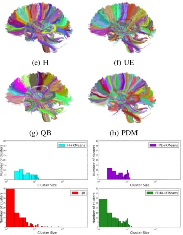
(e) H (f) UE
(g) QB (h) PDM
Figure 3. (top) 560 clusters on brain: Qualitative algorithm comparison for the resulting fiber clusters on an arbitrary chosen subject. (below) Histogram of the cluster sizes for the different algorithms.
chosen subject. Number of fibers was set to 560 for all of them. Resulting clusters on (e), (f) and (g) seem to be wider and more heterogeneous than (h), showing that PDM metric can indeed better capture shape of fibers. Homogeneity of clusters in comparison to (e) (f) and (g) can clearly be seen on the corpus callosum and the corticospinal tract. Below, we can see the histograms on the clusters sizes. We see that QB has the biggest amount of small clusters, that likely correspond to outlier fibers, and it also formed very large clusters. k-means+PDM also seems to generate a few small clusters, in contrary to k-means+H and k-means+UE that have no small clusters, meaning that spurious fibers are included in clusters, and not rejected as outliers.
Both QB and PDM-k-means running time are sensitive to the number of clusters, however QuickBundles’ time com-plexity is O(N Ck) and k-means+PDM O(N Sk2+ N Ck),
where C is the number of clusters, k the fiber resolution and S the sample size. In k-means+PDM, the creation of the partial distance matrix dominates the time complexity as long as Sk > C.
This code has been implemented in Python using utilities provided by Scikit-Learn [8].
V. CONCLUSION
We presented an analysis and comparison of some of the techniques most commonly used on fiber clustering. Believing that clustering can help to simplify the compli-cated structure of brain fibers, we look for homogeneous clusters which can easily be represented by the cluster centroid. We compared the available metrics on the liter-ature for measuring distances between fibers, incorporating PDM which has been used recently to represent geometric structures in the brain, but never for fiber clustering. We show different behaviors of the methods depending on the number of clusters: while QB is good at isolating outlier fibers in small clusters, it requires a large number clusters to represent effectively the whole set of fibers. k-means+PDM has a better compression power, but is less robust against outlier fibers. It clearly outperforms other metrics.
We believe this method along with a posterior fiber registration [5] can be a consistent tool for white matter group analysis. In the future, it could be applied for the analysis of white matter in neurological settings [9].
REFERENCES
[1] E. Garyfallidis et al., “Quickbundles, a method for tractography simplification,” Frontiers in Neuroscience, vol. 6, no. 175, 2012.
[2] B. Moberts et al., “Evaluation of fiber clustering methods for diffusion tensor imaging,” in In IEEE Transactions on VCS, 2005, p. 9.
[3] P. Guevara et al., “Automatic fiber bundle segmentation in massive tractography datasets using a multi-subject bundle atlas,” NeuroImage, vol. 61, no. 4, pp. 1083–1099, 2012.
[4] G. Auzias et al., “Disco: A coherent diffeomorphic framework for brain registration under exhaustive sulcal constraints,” in LNCS, vol. 5761, 2009, pp. 730–738.
[5] V. Siless et al., “Joint T1 and brain fiber log-demons registra-tion using currents to model geometry,” in MICCAI, 2012, pp. 57–65.
[6] C. Fowlkes, S. Belongie, F. Chung, and J. Malik, “Spectral grouping using the nystrom method,” Pattern Analysis and Machine Intelligence, IEEE Transactions on, vol. 26, no. 2, pp. 214–225, 2004.
[7] P. J. Rousseeuw, “Silhouettes: A graphical aid to the interpre-tation and validation of cluster analysis,” JCAM, vol. 20, no. 0, pp. 53 – 65, 1987.
[8] F. Pedregosa et al., “Scikit-learn: Machine learning in Python,” Journal of Machine Learning Research, vol. 12, pp. 2825– 2830, 2011.
[9] L. E. DeLisi et al., “Early detection of schizophrenia by diffu-sion weighted imaging,” Psychiatry Research: Neuroimaging, vol. 148, no. 1, pp. 61 – 66, 2006.