HAL Id: hal-02929946
https://hal.archives-ouvertes.fr/hal-02929946
Submitted on 27 Oct 2020
HAL is a multi-disciplinary open access
archive for the deposit and dissemination of
sci-entific research documents, whether they are
pub-lished or not. The documents may come from
teaching and research institutions in France or
abroad, or from public or private research centers.
L’archive ouverte pluridisciplinaire HAL, est
destinée au dépôt et à la diffusion de documents
scientifiques de niveau recherche, publiés ou non,
émanant des établissements d’enseignement et de
recherche français ou étrangers, des laboratoires
publics ou privés.
The carbon budget of South Asia
P. Patra, J. Canadell, R. Houghton, S. Piao, N.-H. Oh, P. Ciais, K.
Manjunath, A. Chhabra, T. Wang, T. Bhattacharya, et al.
To cite this version:
P. Patra, J. Canadell, R. Houghton, S. Piao, N.-H. Oh, et al.. The carbon budget of South Asia.
Biogeosciences, European Geosciences Union, 2013, 10 (1), pp.513-527. �10.5194/bg-10-513-2013�.
�hal-02929946�
www.biogeosciences.net/10/513/2013/ doi:10.5194/bg-10-513-2013
© Author(s) 2013. CC Attribution 3.0 License.
Biogeosciences
The carbon budget of South Asia
P. K. Patra1, J. G. Canadell2, R. A. Houghton3, S. L. Piao4, N.-H. Oh5, P. Ciais6, K. R. Manjunath7, A. Chhabra7, T. Wang6, T. Bhattacharya8, P. Bousquet6, J. Hartman9, A. Ito10, E. Mayorga11, Y. Niwa12, P. A. Raymond13, V. V. S. S. Sarma14, and R. Lasco15
1Research Institute for Global Change, JAMSTEC, Yokohama 236 0001, Japan
2Global Carbon Project, CSIRO Marine and Atmospheric Research, Canberra, ACT 2601, Australia 3Woods Hole Research Center, 149 Woods Hole Road, Falmouth, MA 02540, USA
4Peeking University, Beijing 100871, China
5Seoul National University, 1 Gwanak-ro, Gwanak-gu, Seoul, South Korea
6IPSL – LSCE, CEA CNRS UVSQ, Centre d’Etudes Orme des Merisiers, 91191 Gif sur Yvette, France 7Space Application Centre, ISRO, Ahmedabad 380 015, India
8National Bureau of Soil Survey and Land use Planning (ICAR) Amravati Road, Nagpur 440 033, India 9Institute for Biogeochemistry and Marine Chemistry, 20146, Hamburg, Germany
10National Institute for Environmental Studies, Tsukuba, Ibaraki 305-8506, Japan 11Applied Physics Laboratory, University of Washington, Seattle, WA 98105, USA 12Meteorological Research Institute, Tsukuba, Japan
13Yale University, New Haven, CT 06511, USA
14National Institute of Oceanography, Visakhapatnam 530 017, India 15The World Agroforestry Centre (ICARF), Laguna 4031, Philippines
Correspondence to: P. K. Patra (prabir@jamstec.go.jp)
Received: 27 August 2012 – Published in Biogeosciences Discuss.: 5 October 2012 Revised: 22 December 2012 – Accepted: 2 January 2013 – Published: 25 January 2013
Abstract. The source and sinks of carbon dioxide (CO2) and methane (CH4) due to anthropogenic and natural bio-spheric activities were estimated for the South Asian re-gion (Bangladesh, Bhutan, India, Nepal, Pakistan and Sri Lanka). Flux estimates were based on top-down methods that use inversions of atmospheric data, and bottom-up meth-ods that use field observations, satellite data, and terres-trial ecosystem models. Based on atmospheric CO2 inver-sions, the net biospheric CO2 flux in South Asia (equiva-lent to the Net Biome Productivity, NBP) was a sink, es-timated at −104 ± 150 Tg C yr−1during 2007–2008. Based on the bottom-up approach, the net biospheric CO2 flux is estimated to be −191 ± 193 Tg C yr−1 during the period of 2000–2009. This last net flux results from the follow-ing flux components: (1) the Net Ecosystem Productivity, NEP (net primary production minus heterotrophic respira-tion) of −220 ± 186 Tg C yr−1 (2) the annual net carbon flux from land-use change of −14 ± 50 Tg C yr−1, which re-sulted from a sink of −16 Tg C yr−1 due to the establish-ment of tree plantations and wood harvest, and a source of 2 Tg C yr−1due to the expansion of croplands; (3) the
river-ine export flux from terrestrial ecosystems to the coastal oceans of +42.9 Tg C yr−1; and (4) the net CO2 emission due to biomass burning of +44.1 ± 13.7 Tg C yr−1. Includ-ing the emissions from the combustion of fossil fuels of 444 Tg C yr−1 for the 2000s, we estimate a net CO2 land– atmosphere flux of 297 Tg C yr−1. In addition to CO2, a frac-tion of the sequestered carbon in terrestrial ecosystems is released to the atmosphere as CH4. Based on bottom-up and top-down estimates, and chemistry-transport modeling, we estimate that 37 ± 3.7 Tg C-CH4yr−1 were released to atmosphere from South Asia during the 2000s. Taking all CO2 and CH4 fluxes together, our best estimate of the net land–atmosphere CO2-equivalent flux is a net source of 334 Tg C yr−1 for the South Asian region during the 2000s. If CH4 emissions are weighted by radiative forcing of molecular CH4, the total CO2-equivalent flux increases to 1148 Tg C yr−1 suggesting there is great potential of reduc-ing CH4emissions for stabilizing greenhouse gases concen-trations.
514 P. K. Patra et al.: The carbon budget of South Asia
1 Introduction
South Asia (Bangladesh, Bhutan, India, Nepal, Pakistan and Sri Lanka) is home to 1.6 billion people and covers an area of 4.5 × 10⁶km2. These countries are largely self-sufficient in food production through a wide range of natural re-sources, and agricultural and farming practices (FRA, 2010). However, due to rapid economic growth, fossil fuel emis-sions have increased from 213 Tg C yr−1 in 1990 to about 573 Tg C yr−1in 2009 (Boden et al., 2011). A detailed bud-get of CO2 exchange between the earth’s surface and the atmosphere is not available for the South Asian region due to a sparse network of key carbon observations such as at-mospheric CO2, soil carbon stocks, woody biomass, and CO2uptake and release by managed and unmanaged ecosys-tems. Only recently, Patra et al. (2011a) estimated net CO2 fluxes at seasonal time intervals by inverse modeling (also known as top-down approach), revealing strong carbon up-take of 149 Tg C month−1during July–September following the summer monsoon rainfall.
The region is also very likely to be a strong source of CH4 due to rice cultivation by an amount that still remains controversial in the literature (Cicerone and Shetter, 1981; Fung et al., 1991; Yan et al., 2009; Manjunath et al., 2011), and large numbers of ruminants linked to religious and farm-ing practices (Yamaji et al., 2003; Chhabra et al., 2009a). Since the green revolution there has been an increase in CH4 emissions owing to the introduction of high-yielding crop species, increased use of nitrogen and phosphorus fertilizers, and expansion of cropland areas to meet the food demands of a growing human population in countries of South Asia (Bouwman et al., 2002; Patra et al., 2012a).
South Asia has also undergone significant changes in the rates of land- use change over the last 20 yr contributing to the net carbon exchange. India alone has increased the extent of forest plantations by 4.5 Mha (∼ 7 % of 64 Mha in 2010) from 1990 to 2010 leading to a 26 % increase in the carbon stock in living forest biomass (FRA, 2010).
In this paper we establish for the first time the net carbon budget of South Asia, including CO2and CH4, and its inter-annual variability for the period 1990–2009. We achieve this goal by synthesizing the results of multiple approaches that include (1) atmospheric inversions as so-called top-down methods, and (2) fossil fuel consumption, forest/soil invento-ries, riverine exports, remote sensing products and dynamic global vegetation models as bottom-up methods. The com-parison of independent and partially independent estimates from these various methods help to define the uncertainty in our knowledge on the South Asian carbon budget. Finally, we attempt to separate the net carbon balance into its main contributing fluxes including fluxes from net primary pro-duction, heterotrophic respiration, land-use change, fire, and riverine export to coastal oceans. This effort is consistent with and a contribution to the REgional Carbon Cycle
As-Fig. 1. Landmass selected for the RECCAP South Asia region following the definition of the United Nations and by accounting for the similarities in vegetation types as shown by the coloured map at 1 × 1ospatial resolution (DeFries and Townshend, 1994).
figure
Fig. 1. Landmass selected for the RECCAP South Asia region
fol-lowing the definition of the United Nations and by accounting for the similarities in vegetation types as shown by the colored map at 1 × 1◦spatial resolution (DeFries and Townshend, 1994).
sessment and Processes (Canadell et al., 2011; Patra et al., 2012b).
2 Materials and methods
The South Asian region designated for this study is shown in Fig. 1, along with the basic ecosystem types (De-Fries and Townshend, 1994). A large fraction of the area is cultivated croplands and grassland or wooded grass-land (1.3 × 10⁶km2 and 1.5 × 10⁶km2 or 0.89 × 10⁶km2, respectively). The rest of the area is classified as bare soil, shrubs, broadleaf evergreen, broadleaf deciduous and mixed coniferous (0.35 × 10⁶km2, 0.22 × 10⁶km2, 0.11 × 10⁶km2, 0.10 × 10⁶km2and 0.05 × 10⁶km2, respec-tively). The region is bounded by the Indian Ocean in the south and the Himalayan mountain range in the north. The meteorological conditions over the South Asian region are controlled primarily by the movement of the inter-tropical convergence zone (ITCZ). When the ITCZ is located over the Indian Ocean (between Equator to 5◦S) during boreal au-tumn, winter and spring, the region is generally dry without much occurrence of rainfall. When the ITCZ is located north of the region, about 70 % of precipitations occur during the boreal summer (June–September). Some of these prevailing meteorological conditions are discussed in relations to CO2 and CH4surface fluxes, and concentration variations in ear-lier studies (Patra et al., 2009, 2011a).
2.1 Emissions from the combustion of fossil fuels and cement production
Carbon dioxide emission statistics were taken from the CDIAC database of consumption of fossil fuels and ce-ment production (Boden et al., 2011). CO2emissions were
derived from energy statistics published by the United Na-tions (2010) and processed according to methods described in Marland and Rotty (1984). CO2emissions from the pro-duction of cement were based on data from the US De-partment of Interior’s Geological Survey (USGS, 2010), and emissions from gas flaring were derived from data provided by the UN, US Department of Energy’s Energy Information Administration (1994), and Rotty (1974).
2.2 Emissions from land use and land-use change
Emissions from land-use change include the net flux of carbon between the terrestrial biosphere and the atmo-sphere resulting from deliberate changes in land cover and land use (Houghton, 2003). Flux estimates are based on a book keeping model that tracks living and dead carbon stocks including wood products for each hectare of land cultivated, harvested or reforested. Data on land-use change was from the Global Forest Re-source Assessment of the Food and Agriculture Organiza-tion (FRA, 2010; http://www.fao.org/forestry/fra/fra2010/en; accessed 15 December 2012). We also extracted in-formation from national communication reports to the United Nations Framework Convention on Climate Change (http://unfccc.int/national reports/items/1408.php; accessed 15 December 2012).
2.3 Fire emissions
Fire emissions for the region were obtained from the Global Fire Emissions Database version 3.1 (GFEDv3.1). GFED is based on a combination of satellite information on fire ac-tivity and vegetation producac-tivity (van der Werf et al., 2006, 2010). The former is based on burned area, active fires, and fAPAR from various satellite sensors, and the latter is esti-mated with the satellite-driven Carnegie Ames Stanford Ap-proach (CASA) model.
2.4 Transport of riverine carbon
To estimate the land to ocean carbon flux, we used the six ocean coastline segments with their corresponding river catchments for South Asia, as described by the COSCAT database (Meybeck et al., 2006). The lateral transport of car-bon to the coast was estimated at the river basin scale using the Global Nutrient Export from WaterSheds (NEWS) model framework (Mayorga et al., 2010), including NEWS basin areas. The carbon species models are hybrid empirically and conceptually based models that include single and multiple linear regressions developed by the NEWS effort and Hart-mann et al. (2009), and single-regression relationships as-sembled from the literature. Modeled dissolved and partic-ulate organic carbon (DOC and POC) loads used here (from Mayorga et al., 2010) were generated largely using drivers corresponding to the year 2000, including observed hydro-climatological forcings, though some parameters and the
ob-served loads are based on data spanning the previous two decades. Total suspended sediment (TSS) exports were also estimated by NEWS. Dissolved inorganic carbon (DIC) esti-mates correspond to weathering-derived bicarbonate exports and do not include CO2supersaturation; the statistical rela-tionships developed by Hartmann et al. (2009) were adjusted in highly weathered tropical soils (ferralsols) to 25 % of the modeled values found in Hartmann et al. (2009) to account for overestimates relative to observed river exports (J. Hart-mann and N. Moosdorf, unpublished data); adjusted grid-cell scale exports were aggregated to the basin scale using NEWS basin definitions (Mayorga et al., 2010), then reduced by applying a NEWS-based, basin-scale consumptive water removal factor from irrigation withdrawals (Mayorga et al., 2010). DIC modeled estimates represent approximately the years 1970–2000. Overall, carbon loads may be character-ized as representing general conditions for the period 1980– 2000. Carbon, sediment and water exports were aggregated from the river basin scale to corresponding COSCAT regions.
2.5 Fluxes by terrestrial ecosystem models
We use the net primary productivity (NPP) and heterotrophic respiration (RH) simulated by ten ecosystem models: HyLand, Lund-Potsdam-Jena DGVM (LPJ), ORCHIDEE, Sheffield–DGVM, TRIFFID, LPJ GUESS, NCAR CLM4C, NCAR CLM4CN, OCN and VEGAS. The models used the protocol as described by the carbon cycle model intercom-parison project (TRENDY) (Sitch et al., 2012; Piao et al., 2012; http://dgvm.ceh.ac.uk/system/files/Trendy protocol% 20 Nov2011 0.pdf), where each model was run from its pre-industrial equilibrium (assumed at the beginning of the 1900s) to 2009. We present net ecosystem productivity (NEP = NPP − RH) from two simulation cases; S1: where models consider change in atmospheric CO2 concentration alone, and S2: where models consider change in climate and rising atmospheric CO2concentration.
The historical changes in atmospheric CO2 concen-tration for the period of 1901–2009 were derived from ice core records and atmospheric observations from the Scripps Institution of Oceanography (Keeling et al., 2001). For the climate forcing datasets, monthly cli-mate data for the period of 1901–2009 from CRU-NCEP datasets with a spatial resolution 0.5◦×0.5◦ (http://dods.extra.cea.fr/data/p529viov/cruncep/) were used. Information on land-use change was derived from HYDE 3.1 land cover dataset (Goldewijk, 2001, ftp.pbl.nl; path: /hyde/hyde31 final). These models do not include lat-eral fluxes of C exported away from ecosystems (from soils to rivers, biomass harvested products) nor fluxes resulting from forest and agricultural management.
We performed correlation analyses between detrended net carbon flux and two climate drivers, annual temperature and annual precipitation, in order to diagnose the modeled inter-annual response of net carbon fluxes to these drivers (positive
516 P. K. Patra et al.: The carbon budget of South Asia
for carbon source, negative for carbon sink). The detrended fluxes were calculated by removing the 30-yr linear trend of each variable (net carbon flux, annual temperature and an-nual precipitation), in order to avoid the confounding effects of the simultaneous trends of temperature or rainfall, with those of other environmental drivers such as rising CO2.
2.6 Atmospheric inverse models
The biospheric (non-fossil CO2) CO2 fluxes are available from state-of-the art atmospheric inversion models from the TransCom database at IPSL/LSCE (http://transcom.lsce.ipsl.fr; Peylin et al., 2012). Estimated fluxes from the following models are included in this analysis: C13 CCAM, C13 CCAM, Carbontracker EU, Jena s96 v3.2, JMA 2010, LSCE an v2.1, LSCE var v1.0, NICAM MRI, RIGC TDI64, TransCom-L3 mean. We also obtained regional specific inversion results for South Asia using the CARIBIC (Schuck et al., 2010) data in the upper troposphere over India and Pakistan, which is subsequently validated using the CONTRAIL (Machida et al., 2008) data of vertical profiles over Delhi and upper troposphere over Asia (Patra et al., 2011a). CONTRAIL observations are also used for inversion, with CARIBIC data for validation (Niwa et al., 2012). Measurements of atmospheric CO2 in the South Asian region are limited to Cabo de Rama, India, for the period of 1993–2002 (Bhattacharya et al., 2009). This site constrains the CO2 fluxes from India during winter to spring seasons only. Thus the use of aircraft measurements is indispensable for top-down flux estimates over the full seasonal cycle.
2.7 Methane fluxes
Top-down estimates: global distributions of CH4emissions
are prepared using site scale field measurements, inventories (in the case of fossil CH4emissions and livestock emissions) and their extrapolation using remote sensing of wetland distribution and terrestrial ecosystem models (e.g. Math-ews and Fung, 1987; Olivier and Berdowski, 2001; Ito and Inatomi, 2012). Components of these bottom-up estimations are scaled and used as an input to chemistry-transport models and compared with atmospheric mixing ratio measurements, or are used as prior flux estimates for inverse modeling of surface CH4fluxes (Patra et al., 2011a; Bousquet at al., 2006 and references therein). Patra et al. (2011b) prepared 6 dis-tinct CH4 budgets; 5 of those being anthropogenic sources (EDGAR, 2010; version 3.2, 4.0) in combination with nat-ural sources due to wetlands (Ringeval et al., 2010; Ito and Inatomi, 2012), biomass burning (van der Werf et al., 2006), and those from Fung et al. (1991), and one being based on inversion of atmospheric concentrations (Bousquet et al., 2006). 1990 1995 2000 2005 2010 0 100 200 300 400 500 600 Fossil fuel CO 2 emission (TgC yr -1 ) Total Bhutan Bangladesh India Nepal Pakistan Sri Lanka
Fig. 2. Time series of CO2emissions due to fossil fuel consumption and cement production from the South Asia region during the period of 1990–2009 (source: Boden et al., 2011).
Fig. 2. Time series of CO2emissions due to fossil fuel
consump-tion and cement producconsump-tion from the South Asian region during the period of 1990–2009 (source: Boden et al., 2011).
Bottom-up estimates for India: methane fluxes for India
were estimated using bottom-up inventory data which relied on SPOT Vegetation NDVI, Radarsat Scan SAR (SN2) and IRS AWiFS to map the different rice lands and generate the feed/fodder area for livestock consumption (Manjunath et al., 2011; Chhabra et al., 2009a).
Methane fluxes are given in the units of TgC-CH4, by ac-counting for the mass of carbon atoms in CH4(1 TgC-CH4 is equivalent to1612Tg of CH4).
3 Results and discussion
3.1 Emissions from fossil fuels and cement production
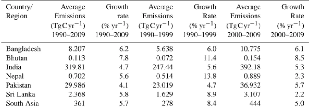
Figure 2 shows the fossil fuel and cement CO2 emissions trends over the South Asian region and member countries over the past two decades (see also Table 1). Growth rates are calculated as the slope of a fitted linear function, nor-malized by the average emissions for the period of inter-est. The average regional total emissions are estimated to be 278 and 444 Tg C yr−1 for the periods of 1990s and 2000s, respectively. The regional total emissions have steadily in-creased from 213 Tg C yr−1in 1990 to 573 Tg C yr−1in 2009. About 90 % of emissions from South Asia are due to fos-sil fuel consumptions in India at a normalized growth rate of 4.7 % yr−1 for the period of 1990–2009. The decadal growth rates do not show large differences between the 1990s (5.5 % yr−1) and 2000s (5.3 % yr−1) for the whole region, while an increased rate of consumptions was observed af-ter 2005 (6.8 % yr−1). This acceleration (Fig. 2) in fossil fuel consumption is largely due to the growth of the Indian econ-omy, where the gross domestic product (GDP) doubled, from 34 trillion Indian Rupees in 2005 to 67 trillion Indian Rupees in 2010 (http://en.wikipedia.org/wiki/Economy of India).
Table 1. Average fossil fuel CO2emissions and annual growth rates (%) for the decades of 1990s, 2000s, and the full RECCAP period (1990–2009).
Country/ Average Growth Average Growth Average Growth
Region Emissions rate Emissions Rate Emissions Rate
(Tg C yr−1) (% yr−1) (Tg C yr−1) (% yr−1) (Tg C yr−1) (% yr−1) 1990–2009 1990–2009 1990–1999 1990–1999 2000–2009 2000–2009 Bangladesh 8.207 6.2 5.638 6.0 10.775 6.1 Bhutan 0.113 7.8 0.072 11.4 0.154 8.5 India 319.81 4.7 247.44 5.6 392.18 5.3 Nepal 0.702 5.6 0.514 13.8 0.889 2.3 Pakistan 29.986 4.1 23.019 4.7 36.932 5.7 Sri Lanka 2.368 5.8 1.629 8.9 3.107 2.2 South Asia 361 5.7 278 8.4 444 5.0
Table 2. Net emissions (+) and accumulations (−) of carbon (Tg C yr−1) attributed to different types of land use in South Asia. Assessment Crops Plantation Industrial Fuelwood Shifting Total
period harvest harvest cultivation
1980–1989 5 −5 2 −4 0 −2
1990–1999 6 −11 −1 −5 0 −11
2000–2010 2 −13 0 −3 0 −14
3.2 Emissions from land-use change (LUC)
The annual net flux of carbon from land-use change in South Asia was a small sink (−11 Tg C yr−1 for the 1990s and −14 Tg C yr−1 for the period 2000–2009) (Table 2). The average sink over the 20-yr period 1990–2009 was
−12.5 Tg C yr−1. Three activities drove this net sink: estab-lishment of tree plantations (−13 Tg C yr−1 in the most re-cent decade), wood harvest (−3 Tg C yr−1), and the expan-sion of croplands (2 Tg C yr−1). Wood harvest results in a net sink of carbon because both industrial wood and fuelwood harvesting have declined recently, while the forest ecosystem productivity remained constant (FRA, 2010).
Tree plantations (eucalyptus, acacia, rubber, teak, and pine) expanded by 0.2 × 10⁶ha yr−1 in the 1990–1999 pe-riod and by 0.3 × 10⁶ha yr−1during 2000–2009 in the region (FRA, 2010). Uptake of carbon as a result of these new plan-tations, as well as those planted before 1990, averaged −11 and −13 Tg C yr−1in the two decades, respectively.
Industrial and fuelwood harvest (including the emissions from wood products and the sink in regrowing forests) was a net sink of −6 and −3 Tg C yr−1in the two decades, most of this sink from fuelwood harvest. The net sink attributable to logging suggests that rates of wood harvest have declined in recent decades, while the recovery of forests harvested in previous years drives a net sink in forests.
The carbon sink in expanding plantations and growth of logged forests was offset only partially by the C source from the expansion of croplands, which is estimated to have re-leased 6 Tg C yr−1and 2 Tg C yr−1during the 1990s and the first decade of 2000, respectively.
The net change in forest area in South Asia was zero for the decade 1990–1999 and averaged 200 000 ha yr−1during 2000–2009 (FRA, 2010). Given the rates of plantation ex-pansion during these decades (200 000 ha yr−1in the 1990– 1999 period and by 300 000 ha yr−1 during 2000–2009), native forests were lost at rates of 200 000 ha yr−1 and 100 000 ha yr−1in the two decades.
The large changes in forest area, both deforestation and afforestation, lead to gross emissions (∼ 120 Tg C yr−1) and a gross uptake (∼ 135 Tg C yr−1) that are large relative to the net flux of 14 Tg C yr−1. Thus, the uncertainty is greater than the net flux itself. The uncertainty is estimated to be 50 Tg C yr−1, a value is somewhat less than 50 % of the gross fluxes.
The net flux for South Asia was determined to a large ex-tent by land-use change (the expansion of tree plantations) in India, which accounts for 72 % of the land area of South Asia, 85 % of the forest area, and > 95 % of the annual in-crease in plantations. Although 11 estimates of the net car-bon flux due to land- use change for India published since 1980 have varied from a net source of 42.5 Tg C yr−1 to a net sink of −5.0 Tg C yr−1. The recent estimates by Kaul et al. (2009) for the late 1990s and up to 2009 suggest a de-clining source/increasing sink (Table 2), consistent with the findings reported here for all of South Asia.
Because India represents the largest contribution to land-use change in South Asia, and becaland-use there have been a number of analyses carried out for India, the discussion below focuses on India. A major theme of carbon budgets for India’s forests has been the roles of tree plantations ver-sus native forests. The 2009 Forest Survey of India (FSI)
Table 3. Estimates of carbon emissions (+) and removals (−) from land-use change in India (from Kaul et al., 2009).
Assessment period Net C release Deforestation Reference (Tg C yr−1) (Mha yr−1)
1980 −3.98 – Hall and Uhlig (1991) 1985 42.52 0.05 Mitra (1992) 1986 −5.00 0.49 Ravindranath et al. (1997) 1987 38.21 1.50 WRI (1990) 1990 0.40 0.06 ALGAS (1998) 1991 5.73 0.34 WRI (1994) 1994 12.8 – Haripriya (2003)
1985–1996 9.0 – Chhabra and Dadhwal (2004)
1994 3.86 – NATCOM (2004) 1982–1992 5.65 0.22 Kaul et al. (2009) 1992–2002 −1.09 0.07 Kaul et al. (2009) 1980–1989 −2 – This study 1990–1999 −11 – This study 2000–2009 −14 – This study
reported a 5 % increase in India’s forest area over the previ-ous decade. This is a net change, however, masking the loss rate of native forests (0.8 % to 3.5 % per year) and a large in-crease in plantations (eucalyptus, acacia, rubber, teak, or pine trees) of ∼ 5700 km2to ∼ 18 000 km2 per year (Puyravaud et al., 2010).
The same theme is evident in the earlier carbon budgets for India’s forests. Ravindranath and Hall (1994) noted that, nationally, forest area declined slightly (0.04 %, or 23 750 ha annually) between 1982 and 1990. At the state level, how-ever, adding up only those states that had lost forests (still an underestimate of gross deforestation), the loss of for-est area was 497 800 ha yr−1 between 1982 and 1986, and 266 700 ha yr−1between 1986 and 1988. These losses were obviously offset by “gross” increases in forest area in other states.
Similarly, Chhabra et al. (2002) found a net decrease of
∼0.6 Mha in total forest cover for India, 1988–1994, while district-level changes indicated a gross increase of 1.07 Mha and a gross decrease of 1.65 Mha. These changes in area translated into a decrease of 77.8 Tg C in districts losing forests and an increase of 81 Tg C in districts gaining forests (plantations) during the same period. It seems odd, though not impossible, that carbon accumulated during this period while forest area declined (Table 3). Clearly, the uncertain-ties are high.
This analysis did not include shifting cultivation in South Asia, but Lele and Joshi (2009) attributed much of the defor-estation in northeast India to shifting cultivation. Houghton (2007) also omitted the conversion of forests to waste lands, while Kaul et al. (2009) attribute the largest fluxes of carbon to conversion of forests to croplands and wastelands. It seems unlikely that forests are deliberately converted to wastelands. Rather, wastelands probably result either from degradation of
croplands (which are then replaced with new deforestation) or from over-harvesting of wood.
Fuelwood harvest, and its associated degradation of car-bon stocks, and even deforestation, seems another primary driver of carbon emissions in South Asia. For example, Tahir et al. (2010) report that the use of fuelwood in brick kilns contributed to deforestation in Pakistan, where 14.7 % of the forest cover was lost between 1990 and 2005.
In Nepal, Upadhyay et al. (2005) attribute the loss of car-bon through land-use change to fuelwood consumption and soil erosion, and Awasthi et al. (2003) suggest that fuelwood harvest at high elevations of Himalayan India may not be sus-tainable. On the other hand, Unni et al. (2000) found that fu-elwood harvest within a 100-km radius of two cities showed both conversion of natural ecosystems to managed ones and the reverse, with no obvious net reduction in biomass. They inferred that the demand for fuelwood on forest and non-forest biomass was not great enough to degrade biomass.
The net sink estimated for South Asia in this study may have underestimated the emissions from forest degradation; logged forests were assumed to recover unless they were con-verted to another use. If wood removals exceed the rate of wood growth, carbon stocks will decline (forest degradation) and may ultimately be lost entirely (deforestation).
3.3 Emissions from fires
South Asia is not a large source of CO2 emission due to biomass burning as per the GFED3.1 (Global Fire Emis-sion Database, verEmis-sion 3.1; van der Werf et al., 2006, 2010). Out of about 2,013 ± 384 Tg C yr−1 of global total emis-sions due to open fires as detected by the various satel-lites sensors, only 47 ± 30 Tg C yr−1(2.3 % of the total) are emitted in the South Asian countries. The average and 1σ standard deviations are calculated from the annual mean
emissions in the period 1997–2009. The total emission is reduced to 44 ± 13 Tg C yr−1 if the period of 2000–2009 is considered. The total fire emissions can be attributed to agriculture waste burning (14 ± 4 Tg C yr−1), deforestation fires (21 ± 11 Tg C yr−1), forest fires (2.6 ± 1.5 Tg C yr−1), savanna burning (4.8 ± 1.9 Tg C yr−1) and woodland fires (1.8 ± 1.0 Tg C yr−1) for the period of 2000–2009. The sea-sonal variation of CO2emissions due to fires is discussed in Sect. 3.7.
Fire emissions due to agricultural activities will be largely recovered through the annual cropping cycles, and emissions from wildfires in natural ecosystems will be also largely recovered through regrowth over multiple decades (unless there is a fire regime change for which we have no evi-dence). For these reasons, carbon emissions from fires from the GFED product will not be used to estimate the regional carbon budget, given that fire emissions associated with de-forestation are already included in the land-use change flux presented in this study. GFED fire fluxes are used to inter-preted interannual variability.
3.4 Riverine carbon flux
The total carbon export from South Asian rivers was 42.9 Tg C yr−1, with COSCAT exports ranging from 0.01 to 33.4 Tg C yr−1for the period of 1980–2000 (Table 4). Con-sidering that about 611 Tg C yr−1is estimated to be released from global river systems (Cole et al., 2007; Battin et al., 2009), rivers in the South Asian region contribute about 7 % of global riverine carbon export, which is more than twice the world average rate (the South Asian region has about 3 % of the global land area). The largest riverine carbon ex-port was observed from the Bengal Gulf COSCAT, which is dominated by the combined Ganges–Brahmaputra discharge. The riverine carbon exports from the other five remaining COSCAT basins were lower by up to two orders of magni-tude, ranging from only 0.01 to 4.4 Tg C yr−1(Table 4).
Because large riverine carbon loads can be due to large basin area, we also provide the basin carbon yield (river-ine carbon load per unit area, excluding PIC). Basin carbon yields varied by a few orders of magnitude, ranging from 0.04 to 18.4 g C m−2yr−1. The largest basin carbon yield was again from the Bengal Gulf COSCAT. However, Laccadive Basin COSCAT and West Deccan Coast COSCAT also re-leased 9.5 and 8.2 g C m−2yr−1, respectively. The global mean terrestrial carbon yield can be calculated by divid-ing the global riverine carbon export of 611 Tg C yr−1 (Auf-denkampe et al., 2011; Battin et al., 2009) by the total land area of 149 million km2, providing a global mean yield of 4.1 g C m−2yr−1. Therefore, the three COSCAT regions in South Asia released more carbon per unit area than the global average. Considering that riverine carbon export is heavily dependent on discharge, this is not surprising since the three COSCAT regions have annual discharge values 40 to 120 %
larger than the global average discharge to the oceans of 340 mm yr−1(Mayorga et al., 2010).
The three COSCAT regions with the largest basin car-bon yields (Bengal Gulf, Laccadive Basin, and West Deccan Coast) also corresponded to the area of highest NPP of South Asia (Kucharik et al., 2010), consistent with areas of culti-vated crops and forested regions (Fig. 1). This suggests that terrestrial inputs of carbon, along with the riverine discharge, are the most significant factors in total riverine transport of carbon.
The relative contribution of DIC (Dissolved Inorganic Car-bon), DOC (Dissolved Organic CarCar-bon), and POC (Partic-ulate Organic Carbon) to the total riverine carbon exports varied depending on the region. The Bengal Gulf COSCAT exported riverine DIC, DOC, and POC of 9.3, 7.0, and 17.1 Tg C yr−1, respectively, demonstrating the strong POC contribution (Table 4). Riverine TSS (Total Suspended Sed-iment) loads and basin yields were also the largest from the Bengal Gulf COSCAT, indicating the strong correlation be-tween POC and TSS.
The carbon emitted by soils to river headstreams can be degassed to the atmosphere as CO2 or deposited into sedi-ment during the riverine transport from terrestrial ecosystem to oceanic ecosystem (Aufdenkampe et al., 2011; Cole et al., 2007). The estimated carbon release to the atmosphere from Indian (inner) estuaries (1.9 Tg C yr−1; Sarma et al., 2012) is relatively small compared to the total river flux of South Asia region. The monsoonal discharge through these estu-aries have a short residence time of OC, which helps the OC matters to be transported relatively unprocessed to the open/deeper ocean. The average residence time during the monsoonal discharge period is less than a day, as observed over the period of 1986–2010, with longest residence time of 7 days for the years of low discharge rate (Acharyya et al., 2012). On an average the processing rate of OC in estuaries is estimated to be 30 % in the Ganga-Brahmaputra river sys-tem in Bangladesh, and the remaining 70 % are stored in the deep water of Bay of Bengal (Galy et al., 2007).
3.5 Modeled long-term mean ecosystem fluxes from biosphere models
Bottom-up estimates from all ten ecosystem models, forced by rising atmospheric CO2 concentration and changes in climate (S2 simulation), agree that terrestrial ecosystems of South Asia acted as a net carbon sink during 1980– 2009. The average magnitude of the sink (NEP) estimated by the ten models is −210 ± 164 Tg C yr−1, ranging from
−80 Tg C yr−1 to −651 Tg C yr−1. Rising atmospheric CO2 alone (S1 simulation) accounts for 89–110 % of the car-bon sink estimated in the CO2+Climate simulations (S2), suggesting a dominant role of the CO2 fertilization effect in driving the regional sink. The decadal average NEPs are −193 ± 136, −217 ± 174 and −220 ± 186 Tg C yr−1, re-spectively, for the 1980s, 1990s and 2000s. The net primary
Table 4. Riverine carbon exports from the COSCAT regions in South Asia as estimated by Global NEWS (TSS: Total Suspended
Sediment; DIC: Dissolved Inorganic Carbon; DOC: Dissolved Organic Carbon; POC: Particulate Organic Carbon; TC: Total Carbon (= DIC + DOC + POC).
COSCAT COSCAT Basin Discharge Discharge TSS DIC DOC POC TC
number ID area load load load load
Unit 106km2 km3yr−1 mm yr−1 Tg yr−1 Tg yr−1 Tg yr−1 Tg yr−1 Tg yr−1 1336 Bengal Gulf 1815 1370 755 3411.7 9.3 7.0 17.07 33.4 1337 East Deccan 1118 270 241 153.7 1.8 1.2 1.33 4.4 Coast 1338 Laccadive Basin 0.121 79 645 47.0 0.4 0.3 0.42 1.2 1339 West Deccan 0.337 160 475 136.4 1.2 0.7 0.85 2.8 Coast 1340 Indus Delta 1389 55 39 13.0 0.8 0.3 0.10 1.2 Coast 1341 Oman Gulf 0.264 1 2 0.7 0.0 0.0 0.01 0.01 Sum 5046 1933 381 37 617 13.6 9.5 19.8 42.9
productivity (NPP) for the same decades are 2117 ± 372, 2160 ± 372 and 2213 ± 358 Tg C yr−1, respectively.
Five of the eight models providing CO2+Climate sim-ulations (S2) show that climate change alone led to a car-bon source of 0.1 Tg C yr−1 to 63 Tg C yr−1 over the last three decades (the difference between simulation S2 and S1); the three other models (OCN, ORC and TRI) show that climate change enhanced the carbon sink by −14, −6 and −4 Tg C yr−1. Such model discrepancies result in aver-age net carbon flux driven by climate change as near neutral (10 ± 22 Tg C yr−1).
3.6 Modeled long-term mean ecosystem fluxes from inversions
Top-down estimates of land–atmosphere CO2 biospheric fluxes (i.e. without fossil fuel emissions, and inclusive of LUC flux and riverine export) are estimated by using at-mospheric CO2concentrations and chemistry-transport els. Results are available from 11 atmospheric inverse mod-els participating in the TransCom intercomparison project with varying time periods between 1988–2008 (Peylin et al., 2012). The inversions were run without any observational data over the South Asian region for most part of the 2000s. Therefore, we place a very low confidence in the TransCom inversion results, and a medium confidence in the results of two additional regional inversions using aircraft measure-ments over the region. The estimated net land–atmosphere CO2 biospheric fluxes from the two regional inversions are −317 and −88.3 Tg C yr−1 (Patra et al., 2011a; Niwa et al., 2012). The range of biospheric CO2 fluxes estimated by the 11 TransCom inversions is −158 to 507 Tg C yr−1, with a median value being a sink of −35.4 Tg C yr−1 with a 1-σ standard deviation 182 Tg C yr−1. The median of the TransCom inversions is chosen for filtering the effect of outliers values. In summary, for this RECCAP carbon budget, we propose as a synthesis of the inversion ap-proach the mean value of the two “best” inversions
us-ing region-specific CO2 data and the median of TransCom models (−147 ± 150 Tg C yr−1). For comparison, the NBP is calculated as −104 ± 150 Tg C yr−1(Top-down biospheric flux–Riverine export; further details of NBP calculation in Sect. 3.10.1).
3.7 Seasonal variability of CO2fluxes
Figure 3 shows the comparisons of carbon fluxes as estimated by the terrestrial ecosystem models (NEP), atmospheric-CO2 inverse models (NBP) and fire emissions as estimated from satellite products and modeling. According to the ecosys-tem and inversion models, the peak carbon release is around April–May, while the peak of CO2 uptake is between July and October. The dynamics as seen by the TransCom (global) inversion models is quite unconstrained due to the lack of at-mospheric measurements in the region. A recent study (Pa-tra et al., 2011a) shows that the peak CO2uptake rather oc-curs in the month of August when inversion is constrained by regional measurements from commercial aircrafts. The months of peak carbon uptake are consistent with regional climate seasonality, i.e., the observed maximum rainfall dur-ing June–August months. This predominantly tropical bio-sphere is likely to be limited by water availability as the av-erage daytime temperatures over this region are always above 20◦C and rainfall is very seasonal.
The peak–trough seasonal cycle amplitudes of NEP sim-ulated by the ecosystem models are of similar magnitude (∼ 300 Tg C yr−1) compared to those estimated by one of the inversions constrained by aircraft data (Patra et al., 2011a). The other regional inversion using atmospheric observations within the region estimated a seasonal cycle amplitude about 50 % greater, mainly due to large CO2release in the months of May and June (Niwa et al., 2012). A denser observational data network and field studies are required for narrowing the gaps between different source/sink estimations.
P. K. Patra et al.: The carbon budget of South Asia 521 -3000 -1500 0 1500 3000 TransCom (Peylin et al., 2012) Patra et al. (2011) Niwa et al. (2012) -3000 -1500 0 1500 3000 CO 2 flux (TgC yr -1 ); South Asia CLM4CN HYL LPJ_GUESS LPJ OCN ORC SDGVM TRI VEGAS CLM4C J F MAM J J A S O N D J F MAM J J A S O N D 0 200 400 600 2007 2008 a. Inverse models b. Ecosystem models c. Fire emissions
Fig. 3. Seasonal cycles of South Asian fluxes (TgCyr−1) as simulated by atmospheric inversions (a, top panel), terrestrial ecosystem models (b, middle panel) and fire emissions modeling (c, bottom panel).
Fig. 3. Seasonal cycles of South Asian fluxes (Tg C yr−1) as simu-lated by atmospheric inversions (a, top panel), terrestrial ecosystem models (b, middle panel) and fire emissions modeling (c, bottom panel).
3.8 Interannual variability of carbon fluxes
Because aircraft CO2 observations over South Asia region are limited to only two years (2007 and 2008), we will ex-clude inverse model estimates from the discussions on inter-annual variability.
All ten terrestrial ecosystem models agree that there is no significant trend in the net carbon flux (positive values mean carbon source, negative values mean carbon sink) over South Asia from 1980 to 2009 (Fig. 4). The estimated net car-bon flux (simulation scenario S2) over South Asia exhibits relatively large year-to-year change among the two simu-lation scenarios. The interannual variation of the 30-yr net carbon flux estimated by the average of the ten models is 63 Tg C yr−1measured by standard deviation, or 30 % mea-sured by coefficient of variation (CV). In fact, the CV of the 30-yr net carbon flux estimated by different models show a large range from 14 % to 166 %, and only two models show a CV of larger than 100 %.
The model ensemble unanimously shows that interannual variations in simulated net carbon flux is driven by the inter-annual variability in gross primary productivity (GPP) rather than that in terrestrial heterotrophic respiration (HR),
sug-18 P. K. Patra et al.: The carbon budget of South Asia
−0.6 −0.4 −0.2 0.0 0.2 0.4 0.6
Net carbon flux anomaly(PgC/yr)
Slp: −0.001PgC/yr, P=0.413 −1.0 −0.5 0.0 0.5 1.0 T emperature anomaly(°C) Slp: 0.033°C/yr, P<0.001 1980 1985 1990 1995 2000 2005 −200 −100 0 100 200 Precipitation anomaly(mm) Slp: 0.78mm/yr, P=0.676
Fig. 4. Interannual variations in net carbon flux (top panel), annual temperature (middle panel) and annual precipitation (bottom panel) over South Asia from 1980 to 2009. Dashed lines show the least squared linear fit with statistics shown in text. Grey area in the top panel shows the range of net carbon flux anomalies estimated by the eleven ecosystem models.
Fig. 4. Interannual variations in net carbon flux (top panel), annual
temperature (middle panel) and annual precipitation (bottom panel) over South Asia from 1980 to 2009. Dashed lines show the least squared linear fit with statistics shown in text. Grey area in the top panel shows the range of net carbon flux anomalies estimated by the eleven ecosystem models.
gesting that variations in vegetation productivity play a key role in regulating variations of the net carbon flux. Similar results were also found in other regions such as Africa (Ciais et al., 2009).
To study the effect of climate change on net carbon flux variations, we performed correlation analyses between trended anomalies of the modeled net carbon flux and de-trended anomalies of climate (annual temperature and an-nual precipitation) over the last three decades (see Meth-ods section). All models predict that carbon uptake decrease or reversed into net carbon source responding to increasing temperature, with two models (LPJ GUESS and VEGAS) showing this positive correlation between temperature and net carbon flux statistically significant (r > 0.4, P < 0.05). Regarding the response to precipitation change, eight of the ten models predict more carbon uptake in wetter years, par-ticularly for LPJ; TRIFFID shows a statistically significant (P < 0.05) negative correlation between precipitation and net carbon flux. Thus, warm and dry years, such as 1988 and 2002, tend to have positive net carbon flux anomalies (less carbon uptake or net carbon release). This further implies that the warming trend and the and non-significant trend in pre-cipitation (Fig. 4) during the last three decades over South Asia might not benefit carbon uptake by terrestrial ecosys-tems, although models do not fully agree on the dominant climate driver of interannual variability in the net carbon flux. Six of the models (NCAR CLM4CN, HyLand, LPJ, OCN, ORCHIDEE and TRIFFID) show interannual variabil-ity in net carbon flux closely associated with variabilvariabil-ity in
precipitation rather than in temperature. The precipitation is also found to be the main driver of seasonal variation in South Asian CO2flux (Patra et al., 2011a).
3.9 Methane emissions
3.9.1 Top-down and bottom-up South Asian CH4
emissions
The South Asian CH4emissions are calculated from 6 sce-narios prepared for the TransCom-CH4 experiment (Patra et al., 2011b). Five of the emission scenarios are constructed by combining inventories of various anthropogenic/natural emissions and wetland emission simulated by a terrestrial ecosystem model (bottom-up), and one is from atmospheric-CH4inversion (top-down). The estimated CH4emissions are in the range of 33.2 to 43.7 Tg C-CH4yr−1 for the period of 2000–2009, with an average value of 37.2 ± 3.7 (1σ of 6 emission scenarios) Tg C-CH4yr−1.
3.9.2 Bottom-up CH4emissions from agriculture in
India – implications for the South Asian budget
Livestock production and rice crop cultivation are the two major sources of CH4emissions from the agriculture sector. The reported emissions due to enteric fermentation and rice cultivation were 6.6 Tg C-CH4yr−1 and 3.1 Tg C-CH4yr−1, respectively, using emission factors appropriate for the re-gion (NATCOM, 2004). India is a major rice-growing coun-try with a very diverse rice growing environment: contin-uously or intermittently flooded, with or without drainage, irrigated or rain fed and drought prone. The average emis-sion coefficient derived from all categories weighted for the Indian rice crop is 74.1 ± 43.3 kg C-CH4ha−1 (Man-junath et al., 2011). The total mean emission (revised estimate) from the rice lands of India was estimated at 2.5 Tg C-CH4yr−1. The wet season contributes about 2.3 Tg C-CH4yr−1amounting to 88 % of the emissions. The emissions from drought-prone and flood-prone regions are 42 % and 18 % of the wet season emissions, respectively.
India has the world’s largest total livestock population with 485 million in 2003, which accounts for ∼ 57 % and 16 % of the world’s buffalo and cattle populations, respec-tively. Methane emissions from livestock have two compo-nents: emission from “enteric fermentation” and “manure management”. Results showed that the total CH4 emission from Indian livestock, including enteric fermentation and manure management, was 11.8 Tg CH4 for the year 2003. Enteric fermentation itself accounts for 8.0 Tg C-CH4yr−1 (∼ 91 %). Dairy buffalo and indigenous dairy cattle to-gether contribute 60 % of the total CH4emission. The three states with high live stock CH4 emission are Uttar Pradesh (14.9 %), Rajasthan (9.1 %) and Madhya Pradesh (8.5 %). The average CH4flux from Indian livestock was estimated at 55.8 kg C-CH4ha−1feed/fodder area (Chhabra et al., 2009a).
The milching livestock constituting 21.3 % of the total live-stock contribute 2.4 Tg C-CH4yr−1 of emission. Thus, the CH4 emission per kg milk produced amounts to 26.9 g C-CH4kg−1milk (Chhabra et al., 2009b).
These CH4 emission estimations of 8.8 Tg C yr−1 from livestock are in good agreement with those of 8.8 (enteric fer-mentation + manure management) Tg C yr−1in the Regional Emission inventory in Asia (REAS) for the year 2000 (Ya-maji et al., 2003; Ohara et al., 2007), while emissions from rice cultivation of 2.5 Tg C yr−1is about half of 4.6 Tg C yr−1, estimated by Yan et al. (2009).
The REAS estimated total CH4 emissions due to anthro-pogenic sources (waste management and combustion, rice cultivation, livestock) from South Asia is 25 Tg C yr−1 for the year 2000, with 6.5, 11.3 and 7.2 Tg C yr−1are emitted due to rice cultivation, livestock and waste management. To match the range of the total flux from South Asia suggested by bottom-up inventories and atmospheric inversions (33.2– 43.7 TgC yr−1), the remaining CH4 sources (mostly natural wetlands and biomass burning) for balancing total emissions from South Asia are in the range of 8–19 TgC yr−1. The com-bination of bottom-up estimations of all CH4sources types from all the member nations with top-down estimates can help close the methane budget in South Asia.
3.10 The carbon budget
3.10.1 Mean annual CO2budget
Figure 5 and Table 5 show the estimates of regional total CO2-carbon emissions from different source types as dis-cussed above. A fraction of the CO2 emissions from fos-sil fuel burning (444 Tg C yr−1, averaged over 2000–2009) is probably taken up by the ecosystem within the region as suggested by the net biome productivity (NBP) esti-mated at −191 ± 193 Tg C yr−1by bottom-up methods, and at −104 ± 150 Tg C yr−1 estimated by top-down methods. The bottom-up NBP is estimated as the sum of terrestrial ecosystem simulated net ecosystem production (NEP), up-take and emissions due to land-use change (LUC), and car-bon export through the river system. The estimated CO2 re-lease due to fires (44 Tg C yr−1) is of similar magnitude than the flux transported out of the land to the coastal oceans by riverine discharge (42.9 Tg C yr−1), but fire emissions are not included in the budget because are largely taken into ac-count in the LUC component. Considering the net balance of these source types (including all biospheric and fossil fuel fluxes of CO2), the South Asian subcontinent is a net source of CO2, with a magnitude in the range of 340 (top-down) to 253 (bottom-up) Tg C yr−1in the period 2000–2009. We choose the mean value of 297 ± 244 Tg C yr−1from the two estimates as our best estimate for the net land–atmosphere CO2flux for the South Asian region.
-400 -200 0 200 400 600 CO 2 flux (TgC yr -1 ) Fossil
NEP1 LUC Fire River NBP2 Fuels NBPG3 NBPR4
Bottom Top Best Best Up5 Down6 Estimate Estimate
CO2 CO2eq Flux Flux
Bottom-up Top-down Net land-to-atmosphere flux
(1) Net Ecosystem Produc2vity (NEP) = NPP – heterotrophic respira2on
(2) Net Biome Produc2vity = Sum of NEP, LUC, Fire, River (NBP = NEP – disturbances and lateral transport) (3) Equivalent to NBP based on global CO2 atmospheric inversions (NBPG)
(4) Equivalent to NBP based on region-‐specific CO2 atmospheric inversions (NBPR) (5) BoPom Up = NBP2 + Fossil Fuel emissions
(6) Top Down = Weighted mean of NBPG3 and NBPR4 + Fossil Fuel emissions (7) Best es2mate CO2 flux (mean of boPom-‐up5 and top-‐down6 es2mates) (8) Best es2mate CO2-‐equivalent (CO2eq) flux that includes CO2 and CH4 fluxes
7 8
Fig. 5. Decadal mean CO2fluxes from various estimates and flux components. The period of estimations differ for source types (ref. Tables 5
and 6 for details).
Table 5. Decadal average CO2fluxes from the South Asian region using bottom-up estimations, top-down estimations and terrestrial
ecosys-tem models. The range of estimate is given as maximum and minimum, and 1-σ standard deviations as the estimated uncertainty or from interannual variability (IAV).
Flux category Flux (Tg C yr−1) Assessment Source period
Fossil fuel +444 (range: +364 to +573) 2000–2009 Boden et al. (2011)
Land-use change −14 ± 50 2000–2009 This study based on Houghton et al. (2007) Open fires +44.1 ± 13.7 (IAV) 2000–2009 GFEDv3.1
Riverine discharge −42.9 1980–2000 This study based on Global NEWS, (DIC + DOC + POC) (Mayorga et al., 2010)
Atmospheric-CO2 −35.4 (model range: 1997–2006 TransCom (Peylin et al., 2012)
inverse model −158 to +507)
Region-specific CO2inversion −317 to −88.3 2007–2008 Patra et al. (2011a), Niwa et al. (2012)
Ecosystem models (NEP) −220 ± 186 2000–2009 Multiple models
3.10.2 The mean annual carbon (CO2+CH4) budget
Table 6 shows the emission and sinks of CO2 and CH4 for the South Asian region. The best estimate of the to-tal carbon or CO2-equivalent (CO2-eq = CO2+CH4) flux is 334 Tg C yr−1, calculated with the average CH4 emis-sions of 37 Tg C yr−1and best estimate of CO2emissions of 297 Tg C yr−1. For this CO2-eq flux, we assumed all CH4is oxidized to CO2 in the atmosphere within about 10 yr (Pa-tra et al., 2011b). However, it is well known that CH4exerts 23 times more radiative forcing (RF) than CO2over a 100-yr
period (IPCC, 2001). For estimating the role of South Asia in global warming, the region contributes RF-weighted CO2-eq emission of 1148 (297 + 37 × 23) Tg C yr−1. The net RF-weight CH4 emission from the South Asian region is more than double of that released as CO2from fossil fuel emis-sions. This result suggests that mitigation of CH4emission should be given high priority for policy implementation. The effectiveness of CH4emission mitigation is also greater due to shorter atmospheric lifetime compared to CO2.
Table 6. Annual fluxes of CO2and CH4(Tg C yr−1). The best-estimate net flux is computed using the mean of top-down and bottom-up
estimates.
Gas species Average fluxes Best estimate RF-weighted CO2-eq
(100 yr horizon) Bottom-up Top-down CO2 −191 ± 186 −104 ± 150 −147 ± 239 (NBP) 297 +444 (fossil fuel) CH4 37.9 ± 3.6 33.2–43.7 37 (total emission) 851 Total 334 1148
4 Future research directions
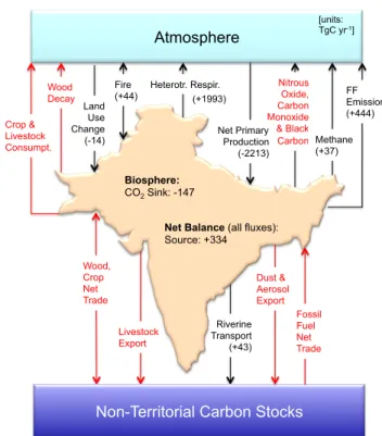
The top-down and bottom-up estimations of carbon fluxes showed good agreement within their respective uncertainties, because we are able to account for the major flow of carbon in to and out of the South Asian region. However, there are clearly some missing flux components that require immedi-ate attention. The fluxes estimimmedi-ated and not estimimmedi-ated in this work are schematically depicted in Fig. 6. Most notably the soil carbon pool and fluxes have not been incorporated in this analysis. The soil organic carbon (SOC) sequestration potential of the South Asian region is estimated to be in the range of 25 to 50 Tg C yr−1 by restoring degraded soil and changing cropland management practices (Lal, 2004). The carbon fluxes associated with international trade (e.g. wood and food products) are likely to be minor contributor to the total budget of South Asia, as the region is not a major ex-porter/importer of these products (FRA, 2010). The region is a major importer of coal and gas for supporting the en-ergy supply (UN, 2010). These flux components, along with several others identified in Fig. 6, will be addressed in the working group of South and Southeast Asian Greenhouse Gases Budget during a 3-yr project of the Asia-Pacific Net-work (2011–2014).
5 Conclusions
We have estimated all major natural and anthropogenic car-bon (CO2 and CH4) sources and sinks in the South Asian region using bottom-up and top-down methodologies.
Excluding fossil fuel emissions and by accounting for the riverine carbon export, we estimated a top-down CO2 sink for the 2000s (equal to the Net Biome Productivity) of
−104 ± 150 Tg C yr−1based on recent inverse model simu-lations using aircraft measurements and the median of multi-model estimates. The flux is in fairly good agreement with the bottom-up CO2 flux estimate of −191 ± 186 Tg C yr−1 based on the net balance of the following fluxes: net ecosys-tem productivity, land-use change, fire, and river export. These results show the existence of a globally modest bio-spheric sink, but a quite significant regionally and per area
20 P. K. Patra et al.: The carbon budget of South Asia
Wood, Crop Net Trade Livestock Export Riverine Transport (+43) Atmosphere
Non-Territorial Carbon Stocks
Biosphere: CO2 Sink: -147 Dust & Aerosol Export Fire (+44) Nitrous Oxide, Carbon Monoxide & Black Carbon Fossil Fuel Net Trade (+1993) Heterotr. Respir. FF Emission (+444) Land Use Change (-14) Wood Decay Crop & Livestock Consumpt. Methane (+37) Net Primary Production (-2213)
Net Balance (all fluxes):
Source: +334
[units: TgC yr-1]
Fig. 6. Schematic diagram of major fluxes of CO2, CH4nitrous oxide (N2O) and related species in South Asia region. The flux components
written in black ink are discussed in this work, and those marked in red ink requires attention for further strengthening our knowledge of regional GHGs budget. Direction of net carbon flow has not been determined well for some of the fluxes, which are represented by lines with arrowheads on both sides.
Fig. 6. Schematic diagram of major fluxes of CO2, CH4 nitrous
oxide (N2O) and related species in the South Asia region. The flux
components written in black ink are discussed in this work, and those marked in red ink requires attention for further strengthening of our knowledge in regional GHGs budget. Direction of net carbon flow has not been determined well for some of the fluxes, which are represented by lines with arrowheads on both sides.
sink driven by the net growth and expansion of vegetation. In a longer time frame, the South Asian sink is also benefiting from the CO2fertilization effect on vegetation growth.
Including fossil fuel emissions, our best estimate of the net CO2 land–atmosphere flux is a source of 297 ± 244 Tg C yr−1 from the average of top-down and bottom-up estimates, and a net CO2-equivalent, including both CO2 and CH4, land–atmosphere flux of 334 Tg C yr−1 for the 2000s. We calculate that the RF-weighted total CH4 emission is 851 Tg C yr−1 from the South Asian region. In
terms of CO2-equivalent flux, methane is largely dominating the budget, at a 100-yr horizon, because of its larger warming potential compared to CO2. This indicates that a mitigation policy for CH4 emission is preferred over fossil fuel CO2 emission control or carbon sequestration in forested land.
Further constraints in the carbon budget of South Asia to reduce current differences between the bottom-up and top-down estimates will require the expansion of atmospheric observations including key isotopes of greenhouse gases and the continuous development of inverse modeling systems that can use a diverse set of data streams including remote sens-ing data. In addition, terrestrial ecosystem models will need to properly represent the crops given the large role of agricul-ture in the region, better constrain the role of wetlands in the methane budget, and expand observations on riverine carbon transport and its ultimate fate in the coastal and open oceans.
Acknowledgements. This work is a contribution to the REgional
Carbon Cycle Assessment and Processes (RECCAP), an activity of the Global Carbon Project. The work is partly supported by JSPS/MEXT (Japan) KAKENHI-A (grant#22241008) and Asia Pacific Network (grant#ARCP2011-11NMY-Patra/Canadell). Canadell is supported by the Australian Climate Change Science Program of CSIRO-BOM-DCCEE. The inverse model results of atmospheric CO2 and terrestrial ecosystem model results
are provided under TransCom (http://transcom.lsce.ipsl.fr) and TRENDY (http://www-lscedods.cea.fr/invsat/RECCAP) projects, respectively, and we appreciate all the modelers’ contribution by providing access to their databases.
Edited by: C. Sabine
References
Acharyya, T., Sarma, V. V. S. S., Sridevi, B., Venkataramana, V., Bharti, M. D., Naidu, S. A., Kumar, B. S. K., Prasad, V. R., Ban-dopadhaya, D., Reddy, N. P. C., and Kumar, M. D.: Reduced river discharge intensify phytoplankton bloom in Godavari estuary, In-dia, Mar. Chem., 132–133, 15–22, 2012.
ALGAS (Asian Lest-Cost Greenhouse Gas Abettment Strategy): Report vol. 4, Asian Development Bank, Manila, 1998. Aufdenkampe, A. K., Mayorga, E., Raymond, P. A., Melack, J. M.,
Doney, S. C., Alin, S. R., Aalto, R. E., and Yoo, K.: Riverine coupling of biogeochemical cycles between land, oceans, and at-mosphere, Front. Ecol. Environ., 9, 53–60, 2011.
Awasthi, A., Uniyal, S. K., Rawat, G. S., and Rajvanshi, A.: Forest resource availability and its use by the migratory villages of Ut-tarkashi, Garhwal Himalaya (India), Forest Ecol. Manag., 174, 13–24, 2003.
Battin, T. J., Luyssaert, S., Kaplan, L. A., Aufdenkampe, A. K., Richter, A., and Tranvik, L. J.: The boundless carbon cycle, Nat. Geosci., 2, 598–600, 2009.
Bhattacharya, S. K., Borole, D. V., Francey, R. J., Allison, C. E., Steele, L. P., Krummel, P., Langenfelds, R., Masarie, K. A., Ti-wari, Y. K., and Patra, P. K.: Trace gases and CO2isotope records from Cabo de Rama, India, Curr. Sci., 97, 1336–1344, 2009.
Boden, T. A., Marland, G., and Andres, R. J.: Global, Regional, and National Fossil-Fuel CO2Emissions (1751–2008) Carbon
Diox-ide Information Analysis Center, Environmental Sciences Divi-sion, Oak Ridge National Laboratory, Oak Ridge, TN 37831– 6290, USA, 2011.
Bousquet, P., Ciais, P., Miller, J. B., Dlugokencky, E. J., Hauglus-taine, D. A., Prigent, C., van der Werf, G. R., Peylin, P., Brunke, E.-G., Carouge, C., Langenfelds, R. L., Lathi´ere, J., Papa, F., Ramonet, M., Schmidt, M., Steele, L. P., Tyler, S. C., and White, J.: Contribution of anthropogenic and natural sources to atmospheric methane variability, Nature, 443, 439–443, 2006. Bouwman, A. F., Boumans, L. J. M., and Batjes, N. H.: Modeling global annual N2O and NO emissions from
fertilized fields, Global Biogeochem. Cy., 16, 1080, doi:10.1029/2001GB001812, 2002.
Canadell J. G., Ciais, P., Gurney, K., Le Qu´er´e, C., Piao, S., Rau-pach M. R., and Sabine, C. L.: An international effort to quantify regional carbon fluxes, EOS, 92, 81–82, 2011.
Chhabra, A. and Dadhwal, V. K.: Assessment of pools and fluxes of carbon in Indian forests, Climatic Change, 64, 341–360, 2004. Chhabra, A., Palria, S., and Dadhwal, V. K.: Spatial distribution
of phytomass carbon in Indian forests, Global Change Biol., 8, 1230–1239, 2002.
Chhabra, A., Manjunath, K. R., Panigrahy, S., and Parihar, J. S.: Spatial pattern of methane emissions from Indian livestock, Cur-rent Sci., 96, 683–689, 2009a.
Chhabra, A., Manjunath, K. R., and Panigrahy, S.: Assessing the role of Indian livestock in climate change, in: The Interna-tional Archives of the Photogrammetry, Remote Sensing and Spatial Information Sciences, XXXVIII Part 8/W3, ISPRS WG VIII/6 – Agriculture, Ecosystem and Bio-diversity–Space Ap-plications Centre (ISRO), Ahmedabad, India Indian Society of Remote Sensing, Ahmedabad Chapter, http://www.isprs.org/ proceedings/XXXVIII/8-W3/, 359–365, 2009b.
Ciais, P., Piao, S.-L., Cadule, P., Friedlingstein, P., and Ch´edin, A.: Variability and recent trends in the African terrestrial carbon balance, Biogeosciences, 6, 1935–1948, doi:10.5194/bg-6-1935-2009, 2009.
Cicerone, R. J. and Shetter, J. D.: Sources of atmospheric methane: measurements in rice paddies and a discussion, J. Geophys. Res., 86, 7203–7209, 1981.
Cole, J. J., Prairie, Y. T. Caraco, N. F., McDowell, W. H., Tran-vik, L. G., Striegl, R. G., Duarte, C. M., Kortelainen, P., Down-ing, J. A., Middelburg, J. J., and Melack, J.: Plumbing the global carbon cycle: integrating inland waters into the terrestrial carbon budget, Ecosystems, 10, 172–185, 2007.
DeFries, R. S. and Townshend, J. R. G.: NDVI-derived land cover classification at global scales, Int. J. Remote Sens., 15, 3567– 3586, 1994.
Emissions Database for Global Atmospheric Research (EDGAR), European Commission, Joint Research Centre (JRC)/Netherlands Environmental Assessment Agency (PBL), release version 4.1, available at: http://edgar.jrc.ec.europa.eu, last access: 30 November 2010, 2010.
FRA: Global Forest Resource Assessment, Food and Agriculture Organization of the United Nations, Rome, 2010.
Fung, I., John, J., Lerner, J., Matthews, E., Prather, M., Steele, L. P., and Fraser, P. J.: Three-dimensional model synthesis of the global methane cycle, J. Geophys. Res., 96, 13033–13065, 1991.
Galy, V., France-Lanord, C., Beyssac, O., Faure, P., Kudrass, H., and Palhol, F.: Efficient organic carbon burial in the Bengal fan sustained by the Himalayan erosional system, Nature, 450, 407– 410, 2007.
Goldewijk, K. K.: Estimating global land use change over the past 300 years: the HYDE database, Global Biogeochem. Cy., 15, 417–433, 2001.
Hall, C. A. S. and Uhlig, J.: Refining estimates of carbon released from tropical land-use change, Can. J. Forest Res., 21, 118–131, 1991.
Haripriya, G. S.: Carbon budget of the Indian forest ecosystem, Cli-matic Change, 56, 291–319, 2003.
Hartmann, J., Jansen, N., D¨urr, H. H., Kempe, S., and K¨ohler, P.: Global CO2consumption by chemical weathering: what is the
contribution of highly active weathering regions?, Global Planet. Change, 69, 185–194, 2009.
Houghton, R. A.: Revised estimates of the annual net flux of carbon to the atmosphere from changes in land use and land manage-ment 1850–2000, Tellus B, 55, 378–390, 2003.
Houghton, R. A.: Balancing the global carbon budget, Annu. Rev. Earth Pl. Sc., 35, 313–347, 2007.
IPCC, Climate Change 2001: The Scientific Basis, Contribution of Working Group I to the Third Assessment Report of the Inter-governmental Panel on Climate Change, edited by: Houghton, J. T., Ding, Y., Griggs, D. J., Noguer, M., van der Linden, P. J., Da, X., Maskell, K., and Johnson, C. A., Cambridge Univ. Press, Cambridge, UK, 881 pp., 2001.
Ito, A. and Inatomi, M.: Use of a process-based model for assessing the methane budgets of global terrestrial ecosystems and evalua-tion of uncertainty, Biogeosciences, 9, 759–773, doi:10.5194/bg-9-759-2012, 2012.
Kaul, M., Dadhwal, V. K., and Mohren, G. M. J.: Land use change and net C flux in Indian forests, Forest Ecol. Manag., 258, 100– 108, 2009.
Keeling, C. D., Piper, S. C., Bacastow, R. B., Wahlen, M., Whorf, T. P., Heimann, M., and Meijer, H. A.: Exchanges of atmospheric CO2and13CO2with the terrestrial biosphere and
oceans from 1978 to 2000, I. Global aspects, SIO Reference Se-ries, No. 01–06, Scripps Institution of Oceanography, San Diego, 88 pp., 2001.
Kucharik, C. J., Foley, J. A., Delire, C., Fisher, V. A., Coe, M. T., Lenters, J. D., Young-Molling, C., Ramankutty, N., Nor-man, J. M., and Gower, S. T.: Testing the performance of a dy-namic global ecosystem model: water balance, carbon balance, and vegetation structure, Global Biogeochem. Cy., 14, 795–825, 2010.
Lal, R.: The potential of carbon sequstration in soils of South Asia, in: Conserving Soil and Water for Society: Sharing Solutions, 13th International Soil Conservation Organisation Conference, Brisbane, paper no. 134, 1–6, July 2004.
Lele, N. and Joshi, P. K.: Analyzing deforestation rates, spatial for-est cover changes and identifying critical areas of forfor-est cover changes in North-East India during 1972–1999, Environ. Monit. Assess., 156, 159–170, 2009.
Machida, T., Matsueda, H., Sawa, Y., Nakagawa, Y., Hirotani, K., Kondo, N., Goto, K., Nakazawa, T., Ishikawa, K., and Ogawa, T.: Worldwide measurements of atmospheric CO2and other trace
gas species using commercial airlines, J. Atmos. Ocean. Tech., 25, 1744–1754, 2008.
Manjunath, K. R., Panigrahy, S., Adhya, T. K., Beri, V., Rao, K. V., and Parihar, J. S.: Methane emission pattern of Indian rice-ecosystems, J. Ind. Soc. Remote Sens., 39, 307–313, 2011. Marland, G. and Rotty, R. M.: Carbon dioxide emissions from
fos-sil fuels: a procedure for estimation and results for 1950–82, Tel-lus B, 36, 232–261, 1984.
Matthews, E. and Fung, I.: Methane emissions from natural wet-lands: global distribution, area, and ecology of sources, Global Biogeochem. Cy., 1, 61–86, doi:10.1029/GB001i001p00061, 1987.
Mayorga, E., Seitzinger, S. P., Harrison, J. A., Dumon, E., Beusen, A. H. W., Bouwman, A. F., Fekete, B. M., Kroeze, C., and van Drecht, G.: Global nutrient export from WaterSheds 2 (NEWS 2): model development and implementation, Environ. Modell. Softw., 25, 837–853, 2010.
Meybeck, M., Durr, H. H., and Vorosmarty, C. J.: Global coastal segmentation and its river catchment contributors: a new look at land-ocean linkage, Global Biogeochem. Cy., 20, GB1S90, doi:10.1029/2005GB002540, 2006.
Mitra, A. P.: Greenhouse Gas Emissions in India – a Preliminary Report, No. 4, Council of Scientific and Industrial Research & Ministry of Environment and Forests, New Delhi, 1992. NATCOM: India’s Initial National Communication to the United
Nations Framework Convention on Climate Change, Ministry of Environment and Forest (MoEF), Govt. of India, New Delhi, 292 pp., 2004.
Niwa, Y., Machida, T., Sawa, Y., Matsueda H., Schuck T. J., Bren-ninkmeijer C. A. M., Imasu R., and Satoh M.: Imposing strong constraints on tropical terrestrial CO2 fluxes using passenger
aircraft based measurements, J. Geophys. Res., 117, D11303, doi:10.1029/2012JD017474, 2012.
Ohara, T., Akimoto, H., Kurokawa, J., Horii, N., Yamaji, K., Yan, X., and Hayasaka, T.: An Asian emission inventory of anthropogenic emission sources for the period 1980–2020, At-mos. Chem. Phys., 7, 4419–4444, doi:10.5194/acp-7-4419-2007, 2007.
Olivier, J. G. J. and Berdowski, J. J. M.: Global emissions sources and sinks, in: The Climate System, edited by: Berdowski, J., Guicherit, R., and Heij, B. J., ISBN 9058092550, A. A. Balkema Publishers/Swets & Zeitlinger Pub., Lisse, The Netherlands, 33– 78, 2001.
Patra, P. K., Takigawa, M., Ishijima, K., Choi, B.-C., Cunnold, D., Dlugokencky, E. J., Fraser, P., Gomez-Pelaez, A. J., Goo, T.-Y., Kim, J.-S., Krummel, P., Langenfelds, R., Meinhardt, F., Mukai, H., O’Doherty, S., Prinn, R. G., Simmonds, P., Steele, P., Tohjima, Y., Tsuboi, K., Uhse, K., Weiss, R., Worthy, D., and Nakazawa, T.: Growth rate, seasonal, synoptic, diurnal variations and budget of methane in lower atmosphere, J. Meteorol. Soc. Jpn., 87, 635–663, 2009.
Patra, P. K., Niwa, Y., Schuck, T. J., Brenninkmeijer, C. A. M., Machida, T., Matsueda, H., and Sawa, Y.: Carbon balance of South Asia constrained by passenger aircraft CO2
measure-ments, Atmos. Chem. Phys., 11, 4163–4175, doi:10.5194/acp-11-4163-2011, 2011a.
Patra, P. K., Houweling, S., Krol, M., Bousquet, P., Belikov, D., Bergmann, D., Bian, H., Cameron-Smith, P., Chipperfield, M. P., Corbin, K., Fortems-Cheiney, A., Fraser, A., Gloor, E., Hess, P., Ito, A., Kawa, S. R., Law, R. M., Loh, Z., Maksyutov, S., Meng, L., Palmer, P. I., Prinn, R. G., Rigby, M., Saito, R.,