HAL Id: hal-01849431
https://hal.inria.fr/hal-01849431
Submitted on 26 Jul 2018
HAL is a multi-disciplinary open access
archive for the deposit and dissemination of
sci-entific research documents, whether they are
pub-lished or not. The documents may come from
teaching and research institutions in France or
abroad, or from public or private research centers.
L’archive ouverte pluridisciplinaire HAL, est
destinée au dépôt et à la diffusion de documents
scientifiques de niveau recherche, publiés ou non,
émanant des établissements d’enseignement et de
recherche français ou étrangers, des laboratoires
publics ou privés.
LBP Channels for Pedestrian Detection
Remi Trichet, Francois Bremond
To cite this version:
Remi Trichet, Francois Bremond. LBP Channels for Pedestrian Detection. WACV , Mar 2018, Lake
Tahoe, United States. �hal-01849431�
LBP Channels for Pedestrian Detection
Remi Trichet
INRIA
[email protected]Francois Bremond
INRIA
[email protected]Abstract
This paper introduces a new channel descriptor for pedestrian detection. This type of descriptor usually selects a set of one-valued filters within the enormous set of all pos-sible filters for improved efficiency. The main claim under-pinning this paper is that the recent works on channel-based features restrict the filter space search, therefore bringing along the obsolescence of one-valued filter representation. To prove our claim, we introduce a 12-valued filter repre-sentation based on local binary patterns. Indeed, various improvements now allow for this texture feature to provide a very discriminative, yet compact descriptor. Filter selection boasting new combination restrictions as well as a reverse selection process are also presented to choose the best fil-ters. experiments on the INRIA and Caltech-USA datasets validate the approach.
1. Introduction
With the rise of automotive, the growing need for behaviour-oriented surveillance and home-monitoring ap-plications, pedestrian detection is one of the computer vi-sion hot topics.
With over a third [5] of the pedestrian literature dedicated to it, features largely contributed to the progresses in the field. Integral channel features [14] are one of the key-stones of this long, bumpy road. In their original work, the authors employs integral images to integrate many cues, such as gradients and colour. Each of these cue is dubbed a channel. The final descriptor is obtained by convolv-ing a set of patches (named filters) with the different cues. By summarizing a swarm of channel region information, it provides a robust and compact descriptor. Due to their efficiency and reasonable detection time, channel features quickly became a reference. Over the years, many exten-sions were proposed, in terms of either speed [13] or per-formance [11, 5, 52, 24, 28, 54].
In all these works, the response of one filter region is sum-marized with one value, by averaging or subtracting means. Despite their low discriminative power, one-valued filters
were originally chosen to explore more deeply the huge amount of possible filters and select the best performing ones. Indeed, the memory consumption bounds the process and the size of the full descriptor is the number of filters times their response size. So, the bigger the full filter re-sponse will be, the harder it will be to search the feature space for the discriminative filters. On the other hand, indi-vidual filter responses would be more discriminative if char-acterized by more values. Moreover, since channel features were first introduced, heuristics [52, 5, 24, 28] have been brought up to narrow down the filter search space.
Therefore, in this paper, we propose to study the trade-off between these two factors and to show through the introduc-tion of a new channel descriptor that several-valued filters can now reliably be extracted.
This new LBP-based channel descriptor outperforms chan-nel features [14] while requiring a fraction of the original LBP memory footprint. Uniform patterns [29] and Haar-based LBP [10] are employed to shrink the filter dimension in accordance to our needs. Also, cell stacking and new fil-ter combination restriction based on proposal window cov-erage are successfully applied. Finally, a more reliable fea-ture selection technique is introduced. Experiments on two major pedestrian detection datasets demonstrate the robust-ness and discriminative power of our LBP-channel descrip-tor compared to the state-of-art.
Our contribution is 2-fold:
• The introduction of LBP-based feature channels. This
descriptor is one-of-a-kind in several respects. Its size is drastically reduced via the use of uniform patterns [29]and Haar-like descriptors [10]. Moreover, the us-age of stacked cell sizes confers to the descriptor an increased discrimination power without changing its overall size.
• We introduce reversed feature selection to construct
a lower dimension final descriptor without harming its discriminability. Also, new coverage-based restric-tions of filter combination allow for a sharper search. The rest of this paper is organized as follows. Section 2 reviews the related work. Section 3 describes in details
the LBP-channel feature while section 4 proves its efficacy through experimentation. Section 5 concludes this docu-ment.
2. Related Work
Since the Viola and Jones first pedestrian detector [34], the most blatant progresses in pedestrian detection concerns features. HoGs [12] are arguably the most promi-nent. These gradient based descriptors, densely extracted over the image at several scales are fast to compute and particularly discriminative for the human detection task. While the bulk of the literature uses this landmark feature, other noticeable work has been produced.
Another section of the literature focuses on adding extra, complementary features to the original HoG ones. In par-ticular, the combination with colour is the first choice. Luv colour patches [16] self-similarity on colour channels [45] have been proposed, leading to substantial improvement. The addition of flow features [45, 36, 54] has also shown success.
More recently, [14] proposed integral channel features. This approach integrates many cues, like colour or gradi-ents, within integral images, and describes any pedestrian proposal with a swarm of convolved patch regions (named
filters) over these cues. Due to its success, this efficient
descriptor had many extensions. [13] improved its speed considerably, [11] quantized the outcome of each filter therefore reducing the final descriptor size while increasing its summarization capabilities. Significant work also focussed on selecting the best filters among the plethora of possibilities. [5] used square filters, [52] combined it with Haar-type filters and cleverly derived their filters from pedestrian body parts templates to reduce the filter search space. Correlation filters [24] efficiently dealt with correlations in the frequency domain whereas [28] learnt the filter bank as the base of a PCA over the training set.
Another recent class of approach [50, 26, 31, 1, 51, 8] extracts features through the training of a deep neural network. the significant performance increase that the resulting features provide has led a drastic shift in the field toward this deep learning approaches. In this domain as well, researchers enforce contextual features learning in a semi-supervised way. [50] use a set of activation maps to learn each layer’s features. [26] train a Restricted Boltz-mann Machine providing both, images and corresponding labels as observed variables in a supervised manner. Finally, [31], independently define and learn 4 distinct pedestrian detection components: feature extraction, de-formation handling, occlusion handling and classification. Ensemble learning has also been harnessed to guide the technique toward more meaningful features. Cascade of deep networks [1], bootstrapped boosted forests [51] and a pool of both, hand-crafted and CNN features [8] have been
employed for this purpose.
3. LBP-based channel extraction
This section describes how our LBP-channel descrip-tor is extracted. We first recall the basics of the LBP de-scriptor and its variants before explaining how we adjust it to the specificities of channel-structured pedestrian de-scription. Finally, the last subsection details our feature se-lection methodology that minimizes the performance loss while shrinking the descriptor size.
3.1. LBP descriptor
Local Binary Patterns are binary descriptors stemming from texture analysis [38]. Despite their high memory im-pact they became a state-of-the-art descriptor for pedestrian detection [46, 38] due to their fast calculation and their good performance for this task. Also, their ability to characterize texture makes them complementary to the HoG edge de-scriptor [46].
The LBP descriptor encapsulates the local intensity varia-tions within the region to describe. Each local binary pat-tern, in the original descriptor, quantizes the intensity val-ues within regions{r} of 3×3 cells, comparing the 8 border cells intensity values to the center one:
LBP (r) = ∑ i=1...8 S(I(C0)− I(Ci))2i S(x) = { 1 if|x| > T 0 otherwise (1)
with T a noise filtering threshold and I(C) the average intensity over the cell C. The 8-bit pattern is then trans-formed into a decimal by binomial weighting. Similarly to HoG [12], an histogram represents the LBP pattern frequen-cies within a block regions b:
h(i) = ∑
r∈b and LBP (r)=i
1 (2)
and the final descriptor concatenates all the histograms computed over a grid of blocks. The original L1-square block normalization works best for most of the applications but is seldomly outperformed by the L2-norm [20].
This original descriptor has been improved in several re-spects since its introduction in computer vision problems. In order to extend the discrimination power of the descriptor [40]extended the LBP to 3-values code. This local trinary pattern (LTP) is respectively quantized to +1 or -1 depend-ing on whether the compared pixel intensities are above or below T ; its value remains 0 otherwise.
are 256 possible values for a typical 8-bit pattern, there-fore leading to 256-valued block histograms. Important work has been achieved in reducing the number of avail-able patterns without loss of discrimination. [29] stated that most patterns occurring in natural images have at most two transitions within their 8 values. They restricted the pat-tern extraction to this LBP subset that they called uniform patterns. [20] further reduced the number of available pat-terns power by considering inverse patpat-terns (with the excep-tions of the informative 00000000 and 11111111 patterns) identical. In [49], authors choose to decompose the neigh-borhood in two sets: diagonal and horizontal plus vertical comparisons. Each of these 4-valued components has only 16 possible values. They then build the two much smaller histograms separately and concatenate them, for a total of 32 values. This strategy allows for a much more compact descriptor with little loss of discriminability.
Inner LBP possible comparisons are not limited to the dif-ferences with the center cell. A significant number of al-ternate neighborhood topologies have been explored, their efficiency depending on the application tested on. Center-symmetric [55, 21] patterns highlight symmetry, center-surround patterns [41] deal with their neighborhood out-skirts and direction. Finally, [22] combined several of them. The original LBP cell size is 1×1 pixels. We found few au-thors experimenting with different cell sizes [20], and none actually stacking the information of several cell sizes within the block histograms.
LBP-channel descriptors have also been proposed. [22] explored it with a variety of color and contrast channels, as well as different topologies. Their use however provided a limited success compared to channel features [14] as the amount of channels and topologies they could search was limited by the high memory size of the descriptor. This shortcoming was emphasized by the high sparsity of the initial descriptor and a fixed block grid topology. mCEN-TRIST [49] is another multi-channel LBP-based descriptor that tried to capture the complementary information across channels.
3.2. LBP-channel descriptor
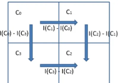
This work gets down to developing a light-weight, al-though more discriminative, channel-based LBP descriptor. Its extraction pipeline is presented in figure 2. As the LBP large memory size impacts the feature exploration capaci-ties, several actions are undertaken to shrink the possible number of patterns. First, we use the Haar-like descriptors [10]topology to LBPs. The feature is composed of 4 cells of size (w, h) instead of the 9 original LBP cells. The feature is then calculated as the concatenated quantization between all adjacent vertical and horizontal cells:
Figure 1: Haar−LBP pattern divided in 4 cells. The arrows depict the 4 operation used to computer the Haar-LBP de-scriptor.
Figure 2: LBP Channel features pipeline.
HLBP (r) = ∑ q=0...3 S(I(Ci)− I(Cj))2q S(x) = { 1 if|x| > T 0 otherwise (3)
With only 16 possible patterns, this more compact repre-sentation allows for a lower memory footprint. This type of topology also allows smaller regions (with a minimal size of 2× 2 pixels), making it a better fit to characterize small pedestrian proposals. Uniform pattern [29] restrictions are systematically applied to further reduce the number of pos-sible patterns to 12, therefore producing a descriptor of di-mensionality similar to HoG [12].
We also substantially improved the descriptor robustness by stacking the frequencies of cells Ciwith various
dimen-sions within the block histograms. A block histogram bin value is then defined as:
h(i) = ∑ i=0...n ( ∑ rCi∈ b and HLBP (rCi) = i 1 ) (4)
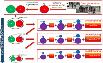
Figure 3: Training pipeline. The initial training set generation selects data while balancing negative and positive sample car-dinalities. A cascade of classifiers is then trained on it, each independent classifier be-ing learnt through bootstrappbe-ing. balanced positive and negative sets is sought all along the cascade. Each circle surface is propor-tional to the set’s cardinality that it repre-sents.
deals efficiently with the pattern deformations within each block, therefore reinforcing the overall descriptor robustness.
For each channel, the feature is computed on a lattice of blocks. An histogram of pattern frequencies is further cal-culated for each block. All the block histograms are finally concatenated to form the final descriptor. The best results are obtained by performing a L1 square normalization on blocks and a L2-normalization on the final histogram.
3.3. Training protocol
Training is performed according to the FairTrain [42] training set generation protocol. The methodology, illus-trated in figure 3, decomposes in two distinct parts: The initial training set generation and the classifier training. The initial training set generation carefully selects data from a set of images while balancing negative and positive sample cardinalities. We then train a cascade of 1 to n clas-sifiers. This cascade could include a cascade-of-rejectors [11, 56, 6, 39, 44], a soft cascade [30], or both. In addition, each independent classifier is learnt through bootstrapping [12, 19]to improve performance. One key aspect is to seek balanced positive and negative sets at all time. Hence, all along the cascade, the minority class is oversampled to create balanced positive and negative sets. See [42, 43] for details.
3.4. Reversed feature selection
Filters are determined according to a pre-defined dense lattice of regularly spaced positions {(xi, yi)}, as well as
sets of width {wj} and heights {hk}. The filter set is the combination of all possible positions and dimensions
{[(xi, yi), wj, hk]} with respect to a 3/1 or higher aspect
ra-tio.
To search this vast amount of possible filter positions and
dimensions {[(xi, yi), wj, hk]} is a complex, often
under-optimal task, and experience has shown that heuristics [52, 5, 24, 28] can help narrow down this search to the most discriminant ones. One key insight in this paper is drown from the following observation: The retained filter set always covers over 95% of the proposal window sur-face. Hence, To drastically restrict the possible number of filter combination to explore, we enforce a filter repartition across the positions {(xi, yi)}. More precisely, with |N| and|P | respectively being the desired number of filters and the number of positions, the amount of filters extracted per position is within the range [1, (|N|/|P |) + 2].
Filters are typically selected using the soft cascade [30]. This algorithm trains a cascade of n classifiers Ci, each of
them being trained by adding the best filter to the feature set. In this paper, we claim that, despite its efficiency, the soft cascade is intrinsically flawed [43]. Indeed, classifiers with few descriptor values lack robustness and adding iter-atively the best features may lead to an under-optimal final descriptor as the combination of features might be more im-portant than their individual efficiency. So, in this work, we instead optimize for the best filter combination. To this end, we build the soft cascade in a reverse way. Let’s define F and Ni as, respectively, the full filter set and the retained
filter set for classifier i. We first train the final classifier harnessing Nnfilters and iteratively train the previous
clas-sifiers by reducing the retained filter set|Ni−1| = |Ni|/2 and updating the full set F = Ni.
When training each classifier Ci, the best filter
combina-tion Niis determined through an expectation-maximisation
(EM) algorithm. Weights, initialized equal, are associated to each filter. At each EM iteration it E-step, the used filter set Nit
i is determined as a weighted draw without
replace-ment over the full filter set F . During the M-step, a clas-sifier is trained on these features and validated on a third party set. The weights of the tested filters are then updated according to the classification score. For a given iteration,
a filter’s weight is then the average classifier performance over all the past runs for which it was selected:
W (xi) = ∑ Sx=[it|x∈Niit] score(Ciit) /|Sx| (5) Unlike the soft-cascade that selects features one by one, this algorithm selects them ”as a all” and, as shown in the experiment section, leads to more robust feature selection. Pseudo-code 1 details the algorithm mechanism.
Data: - A full set of filters S
- The desired number of filters to retain N - The number of classifiers n in the cascade Result:trained classifiers Ciand selected filter Ni
for i=1...n determine the filter set S;
|Nn| ← N;
// Reverse training of n classifiers.
for i=n; i>0; i– do
Ni← EM train(Ci, Ni, F ); |Ni−1| ← |Ni|/2;
F ← Ni; end
// E-M training of classifiers Cifor|Ni| filters with filter set F .
Function EM train(Ci, Ni, F )
Set weights to 1; for j=n; j<#It; j++ do // E-step Ni← draw filters(F , Ni, W ); score← train(Ci, Ni); // M-step update weights(score, W ); end return Ni;
Algorithm 1:Reverse filter selection algorithm. implementation details: Compared to soft-cascade training, where each cascade stage adds one feature to the feature pool, our approach trains many full-feature size de-scriptor, which is time consuming and wouldn’t be track-table on large datasets. So, to speed-up the EM-process, the first iterations are trained with a limited number of trees and bootstrapping data addition and these two parameters are quadratically increased along the iterations until the de-sired number of trees and data addition is reached for the last iterations. More specifically, these parameters are mul-tiplied by (j/#It)2, with j the current iteration and #It the total number of iterations. Moreover, the process is multi-threaded for further boost. All these improvements acceler-ate the algorithm by 2 order of magnitude.
4. Experiments
This section, dedicated to our experimental validation, breaks down into several sub-parts. After presenting the datasets and the experimental setup details, we run individ-ual experiments on the LBP-channel main parameters. The last part compares our work to the state-of-the-art.
4.1. Datasets
We experimented on the INRIA and Caltech-USA datasets. The INRIA [12] features high resolution pictures mostly gleaned from holidays photos. The training set con-sists of 2416 cropped positive instances from 614 images and 1218 images free of persons. The test set contains 1132 positive instances from 288 images and 453 person free im-ages for testing purposes. This is among the most widely used dataset for person detector validation and compara-tive performance analysis. Despite its small size compared to more recent benchmarks, the INRIA dataset boasts high quality annotations and a large variety of angles, scenes, and backgrounds.
The Caltech-USA [17] dataset consists of 2.3 hours of video recorded at 30fps from a vehicle driving various Los Angeles streets. It totals 350000 images and 1900 unique individual pedestrians, 300 large groups, and 110 hard to distinguish pedestrians. Despite some annotation errors [53], its large size along with crowded environments, tiny pedestrians (as low as 20 pixels), and numerous occlusions probably make the Caltech-USA dataset the most widely used one. Annotations allow to experiment on 2 different sets. Contrarily to the ”full set”, the ”reasonable set” re-stricts algorithms to pedestrians over 50 pixels in size and a maximum of 35% occlusion.
With respectively a large variability and tiny occluded detections, everyday pictures and automotive application, these two datasets offer complementary settings for our ex-periments.
4.2. Evaluation protocol
Candidates are selected using a multi-scale sliding win-dow approach [56] with a stride of 4 pixels. Approximately 60% are loosely filtered according to ”edgeness” and sym-metry. No background subtraction or motion features are employed on the Caltech dataset.
The training set size is up-bounded at 12K samples. In-creasing this threshold doesn’t improve performance. No generative resampling is performed. The validation set in-cludes 240K samples for all experiments. The model height is set to 120 pixels for the INRIA dataset, 80 pixels for Cal-tech.
We train a cascade of 6 Adaboost classifiers with a con-stant threshold of 0.56 and a tree depth of 2. We utilised the openCV implementation for the Adaboost classifiers. Ad-aboost is initialised with 256 weak classifiers. Each extra
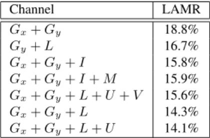
Channel LAMR Gx+ Gy 18.8% Gy+ L 16.7% Gx+ Gy+ I 15.8% Gx+ Gy+ I + M 15.9% Gx+ Gy+ L + U + V 15.6% Gx+ Gy+ L 14.3% Gx+ Gy+ L + U 14.1%
Table 1: Full LBP-descriptor log-average miss rate perfor-mance (the lower the better) on the INRIA dataset when us-ing various channel combinations. I - Grayscale intensity.
{Gx, Gy} gradients respectively along x and y axis. M -gradient magnitude.{L, U, V} - Luv color channels.
Cells LAMR {(3,1); (1,3); (4,4)} 16.3% {(1,1)} 16.0% {(1,2); (2,1); (2,2)} 15.4% {(1,2); (2,1); (2,2); (3,1); (1,3)} 15.2% {(1,1); (1,2); (2,1); (2,2)} 14.7% All 14.1%
Table 2: Full LBP-descriptor log-average miss rate perfor-mance (the lower the better) on the INRIA dataset when using various cell set. Gx+ Gy+ L + U channels are
em-ployed for this experiment.
run adds 64 weak classifiers. This is a low number of weak classifiers compared to typical settings (i.e. [1024, 2048]). However, in practice, increasing this value leads us to lower performance and speed. When employed, reverse feature selection applies to the first 2 classifiers of the cascade, their number of trees being then learnt during training.
We use the threshold variant of non-maximum suppres-sion (t-NMS) [7] that groups the detections according to the bounding boxes overlap with the group d best candidate, keeps the d candidates with highest confidence for each group, and builds the final candidate position with the group mean border positions. We set the overlap threshold to 0.5 and d = 3 for all our experiments. Log-Average Miss Rate (LAMR) [33] is employed as metric for all runs.
4.3. LBP channel setup
For each detection proposal window, the LBP descriptor blocks are spaced out over 8×16 positions along the x and y axis, leading to 128 different possible positions. This lattice allows blocks to be placed approximately every 2 pixels for the smallest Caltech detections and such precision is not useful for bigger pedestrian. The possible filter dimensions wj and hk are {2W/7, 3W/7, 4W/7},
with W the detection window width. In addition to that, filters covering the head, the torso, the legs and the entire
feature selection # Features LAMR Speed(CPU/GPU)
unselected features 373 41.0% 0.3fps soft-cascade 50 39.9% 2.2fps soft-cascade 100 39.8% 1.5fps soft-cascade 150 39.3% 1.2fps undirected selection 150 37.6% 0.7fps reverse selection 50 39.8% 0.8fps reverse selection 100 37.1% 0.8fps reverse selection 150 35.9% 0.7fps
Table 3: Comparison of soft-cascade with reverse feature selection on the LBP-descriptor. Results are in terms of log-average miss rate performance (the lower the better) on the INRIA dataset. Gx+ Gy+ L channels are employed for
this experiment. See text for the methods description.
body are extracted based on edge templates [52], leading to a total of 373 possible filters per channel. In these experiments, the full descriptor will refer to the full set of filter positions with the smallest dimensions 2W/7 only. With this setting, 133 filters, totalling 1596 feature values, are extracted per channel. L1 square block as well as L2 full histogram normalisation are performed in every case.
On the Caltech dataset, the training of the full descriptor and classifiers takes 14 hours; the training of the reduced descriptor takes 17-24 hours with 12 cores assigned to the process. reversed feature selection runs for 200 iterations.
We tested the LBP-channel descriptor with the following 7 channels: graylevel intensities I, gradient magnitude M , gradient along x and y axis Gxand Gy, as well as the L, U and V color channels. We purposely added gradient
channels to explicitly counterbalance this descriptor’s known weak characterization of edges. The combination of various channel has been a assessed on the INRIA dataset. Also, The L, U and V channels are considered separately. Results are displayed on table 1. The gradients Gx, Gy, L, and U channels stand out as the most discriminative.
It also confirms that the grayscale intensity bears much less information than the Luv color channel. The gradient magnitude M and the V color channel are apparently detrimental to the classification.
In our implementation, we experimented with the follow-ing cell dimensions: {(1,1); (1,2); (2,1); (2,2); (1,3); (3,1); (4,4)}. and ran experiments with different combinations of them. Results are displayed on table 2. Of course the more patterns, the better the performance. But this experiment also reveals that the smallest cells are more discriminative, with the detection rate being almost the same when using {(1,1); (1,2); (2,1); (2,2)} cells or the full pattern set. This is sensible as they are the majority to be extracted within small detections, few of their bigger counterparts then fitting within the reduced-sized filters. Finally, it demonstrates the efficiency of stacking cells,
Method INRIA Speed(CPU/GPU)
HoG [12] 46% 0.5fps
HoG-LBP [47] 39% Not provided
MultiFeatures [48] 36% < 1fps FeatSynth [2] 31% < 1fps MultiFeatures+CSS [45] 25% No Channel Features [14] 21% 0.5fps FPDW [13] 21% 2-5fps DPM [18] 20% < 1fps RF local experts [27] 15.4% 3fps PCA-CNN[23] 14.24% < 0.1fps CrossTalk cascades [15] 18.98% 30-60fps VeryFast [3] 18% 8/135fps WordChannels [11] 17% 0.5/8fps SSD[25] 15% 56fps LBP-Channels full 14.3% 0.5/7.5fps LBP-Channels selected 13.6% 0.7/10fps FRCNN[37] 13% 7fps RPN+PF[51] 7% 6fps
Method CALETCH Speed(CPU/GPU)
HoG [12] 69% 0.5fps DPM [18] 63.26% < 1fps FeatSynth [2] 60.16% < 1fps MultiFeatures+CSS [45] 60.89% No FPDW [13] 57.4% 2-5fps Channel Features [14] 56.34% 0.5fps Roerei [4] 48.35% 1 fps MOCO [9] 45.5% < 1fps JointDeep [32] 39.32% < 1fps SquaresChnFtrs [5] 34.8% < 1fps InformedHaar [52] 34.6% < 0.63fps Spatial pooling [35] 29.2% < 1fps Checkboards [54] 24.4% < 1fps FRCNN[37] 56% 7fps CrossTalk cascades [15] 53.88% 30-60fps WordChannels [11] 42.3% 0.5/8fps LBP-Channels full 39.1% 0.5/7.5fps LBP-Channels selected 35.9% 0.7/10fps SSD[25] 34% 56fps RPN+PF[51] 10% 6fps
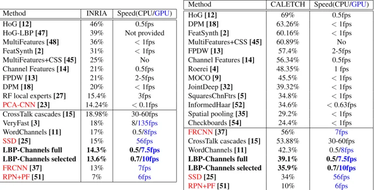
Table 4: Comparison with the state-of-the-art. Near real-time methods are separated from others. Ours is in bold. Deep learning techniques are in red. Computation times are calculated according to 640×480 resolution frames. Gx+ Gy+ L
channels are employed for this experiment. The used metric is the log-average miss rate (the lower the better). Best viewed in color.
results improving from 16.0% to 14.3% when adding extra cells to the (1, 1) base one.
4.4. Results and analysis
Reverse feature selection is compared to soft-cascade in table 3. The main difference with typical feature selection in our case is that 12-valued feature blocks are selected. We select the filter across channels rather than for one channel, which gives us a better performance in practice. The full set of unselected features is provided as baseline and scores 41.0%. During the training phase, the best reverse selec-tion results (reported in this table) are often obtained for the highest number of trees and amount of data added dur-ing bootstrappdur-ing, which confirms the common sense ad-vocating for more trees and data for better performance. If the soft-cascade is faster (running up to 2.2 fps) than re-verse feature selection, it doesn’t provide as discriminative features as the reverse feature selection, with only 1.7% im-provement over the baseline. Comparatively, reverse feature selection provides at best a 5.1% performance boost while running at 0.7 fps. The ”Undirected selection”, referring to the same strategy crippled of the EM-algorithm, shows the overall positive impact of directing the selection process to-ward the best feature blocks, with a 1.8% performance
in-crease. Overall, this strategy seems to learn a better infor-mation structure since the performance steadily increases with the addition of features, contrarily to the soft-cascade that quickly reaches a plateau (around 50 features). How-ever, this is a rather small improvement compared to other channel feature selection methods [5, 52, 35, 54]. We be-lieve that substantial further improvement can be obtained in that direction. The computation time gain remains low even for few features selected because most of the compu-tation lies in the integral channel calculation.
Comparison with the state-of-the-art is presented in table 4. For fair comparison, methods using optical flow features [5, 45, 36, 54], are reported without optical flow or left out of this evaluation. Gx+ Gy+ L channels are employed for
this experiment, giving us a better performance/speed ratio. While running at a similar speed, LBP-channel (full) features greatly outperforms the common channel features [14], scoring 7% better on the INRIA dataset and 16.2% better on the Caltech dataset. Besides the predominance of our descriptor, it shows that one-valued filter responses should not be the de facto choice: A balance between the amount of filters and their response size must be struck. Our reverse feature selection scheme (using 150 feature blocks across channels) further improves the results down to 13.6% on INRIA and 35.9% on CalTech while making it slightly
faster.
Overall, LBP-channels ranks on par or better compared to state-of-the-art pedestrian descriptors in terms of perfor-mance/speed ratio, except for [51]. Deep learning technique [25, 37] often perform better but are slower. The detector speed is, of course, largely influenced by the descriptor pa-rameters, which are the number of filters and channels.
5. Conclusion
In this work, we have presented a new channel descrip-tor based on LBPs. Stacking various cell dimensions and wise channel choices demonstrated the improved descriptor robustness and discriminability. Also, reduced block his-togram size as well as a reverse feature selection alternative to the soft cascade allowed us to efficiently yield a robust set of features. Experiments show that LBP-Channels out-perform their main competitors while still producing a fast and compact descriptor.
Through the introduction of this new descriptor, this paper suggests that there is a balance to strike between the number of feature values used as filter response and the size of the filter space to search. Thorough study should be undertaken to determine what the appropriate trade-off is. These first feature selection results compared to the state-of-the-art im-ply that further research in this particular direction may lead to improved performance.
References
[1] A. Angelova, A. Krizhevsky, V. Vanhoucke, A. S. Ogale, and D. Ferguson. Real-time pedestrian detection with deep net-work cascades. pages 32–1, 2015.
[2] A. Bar-Hillel, D. Levi, E. Krupka, and C. Goldberg. Part-based feature synthesis for human detection. ECCV, 2010. [3] R. Benenson, M. Mathias, R. Timofte, and L. V. Gool.
Pedes-trian detection at 100 frames per second. CVPR, 2013. [4] R. Benenson, M. Mathias, T. Tuytelaars, and L. V. Gool.
Seeking the strongest rigid detector. CVPR, 2013.
[5] R. Benenson, M. Omran, J. Hosang, and B. Schiele. Ten years of pedestrian detection, what have we learned? ECCV,
CVRSUAD workshop, 2014.
[6] B. Berkin, B. K. Horn, and I. Masaki. Fast human detec-tion with cascaded ensembles on the gpu. IEEE Intelligent
Vehicles Symposium, 2010.
[7] M. D. Buil. Non-maximum suppression. technical report
ICG-TR-xxx, 2011.
[8] Z. Cai, M. Saberian, and N. Vasconcelos. Learning complexity-aware cascades for deep pedestrian detection. pages 3361–3369, 2015.
[9] G. Chen, Y. Ding, J. Xiao, and T. X. Han. Detection evo-lution with multi-order contextual co-occurrence. CVPR,
2013.
[10] E. Corvee and F. Bremond. Haar like and lbp based fea-tures for face, head and people detection in video sequences.
ICVS, 2011.
[11] A. D. Costea and S. Nedevschi. Word channel based multi-scale pedestrian detection without image resizing and using only one classifier. CVPR, 2014.
[12] N. Dalal and B. Triggs. Histograms of oriented gradients for human detection. CVPR, 2005.
[13] P. Dollar, S. Belongie, and P. Perona. The fastest pedestrian detector in the west. BMVC, 2010.
[14] P. Dollar, Z. Tu, P. Perona, and S. Belongie. Integral channel features. BMVC, 2009.
[15] P. Dollr, R. Appel, and W. Kienzle. Crosstalk cascades for frame-rate pedestrian detection. ECCV, 2012.
[16] P. Dollr, S. Belongie, and P. Perona. The fastest pedestrian detector in the west. BMVC, 2010.
[17] P. Dollr, C. Wojek, B. Schiele, and P. Perona. Pedestrian detection: A benchmark. CVPR, 2009.
[18] P. Felzenszwalb, R. Girshick, D. McAllester, and D. Ra-manan. Object detection with discriminatively trained part-based models. PAMI, 32(9):1627–1645, 2009.
[19] P. F. Felzenszwalb, R. B. Girshick, and D. McAllester. Cas-cade object detection with deformable part models. CVPR, 2010.
[20] P. Geismann and A. Knoll. Speeding up hog and lbp features for pedestrian detection by multiresolution techniques. ISVC, 2010.
[21] M. Heikkil, M. Pietikinen, and C. Schmid. Description of interest regions with center-symmetric local binary patterns.
Pattern Recognition, 42(3):425–436, 2009.
[22] C. K. Heng, S. Yokomitsu, Y. Matsumoto, and H. Tamura. Shrink boost for selecting multi-lbp histogram features in ob-ject detection. CVPR, 2012.
[23] W. Ke, Y. Zhang, P. Wei, Q. Ye, and J. Jiao. Pedestrian de-tection via pca filters based convolutional channel features.
ICASSP, 2015.
[24] H. Kiani. Multi-channel correlation filters for human action recognition. ICIP, 2014.
[25] W. Liu, D. Anguelov, D. Erhan, C. Szegedy, S. Reed, C.-Y. Fu, and A. C. Berg. Ssd: Single shot multibox detector.
ECCV, 2016.
[26] P. Luo, Y. Tian, X. Wang, and X. Tang. Switchable deep network for pedestrian detection. pages 899–906, 2014. [27] J. Marin, D. Vazquez, A. M. Lopez, J. Amores, and B. Leibe.
Random forests of local experts for pedestrian detection.
ICCV, 2013.
[28] W. Nam, P. Dollar, and J. H. Han. Local decorrelation for improved pedestrian detection. NIPS, 2014.
[29] T. Ojala, M. Pietikainen, and T. Maenpaa. Multiresolution gray-scale and rotation invariant texture classification with local binary patterns. PAMI, 2002.
[30] T. Ojala, M. Pietikinen, and D. Harwood. A comparative study of texture measures with classification based on feature distributions. Pattern Recognition, 29(3):51–59, 1996. [31] W. Ouyang and X. Wang. Joint deep learning for pedestrian
detection. pages 2056–2063, 2013.
[32] W. Ouyang and X. Wang. Joint deep learning for pedestrian detection. ICCV, 2013.
[33] D. P, C. Wojek, B. Schiele, and P. Perona. Pedestrian detec-tion: An evaluation of the state of the art. PAMI, 34(4):743– 761, 2012.
[34] M. J. P. Viola. Robust real-time face detection. IJCV, 2004. [35] S. Paisitkriangkrai, C. Shen, and A. van den Hengel.
Strengthening the effectiveness of pedestrian detection with spatially pooled features. ECCV, 2014.
[36] D. Park, C. Zitnick, D. Ramanan, and P. Dollr. Explor-ing weak stabilization for motion feature extraction. CVPR, 2013.
[37] S. Ren, K. Hen, R. Girshick, and J. Sun. Faster r-cnn: To-wards real-time object detection with region proposal net-works. NIPS, 2015.
[38] B. T. S.Hussain. Feature sets and dimensionality reduction for visual object detection. BMVC, 2010.
[39] M. Souded and F. Bremond. Optimized cascade of classi-fiers for people detection using covariance features. VISAPP, 2013.
[40] X. Tan and B. Triggs. Enhanced local texture feature sets for face recognition under difficult lighting conditions, transac-tions in image processing. ISVC, 19(6):1635–1650, 2010. [41] J. Trefny and J. Matas. Extended set of local binary patterns
for rapid object detection. CWWW, 2010.
[42] R. Trichet and F. Bremond. Dataset optimisation for real-time pedestrian detection. rapport de recherche INRIA 9084, 2017.
[43] R. Trichet and F. Bremond. How to train your dragon: best practices in pedestrian classifier training. IEEE Transactions
on Systems, Man, and Cybernetics: Systems, 2017.
[44] Viola and M. Jones. Rapid object detection using a boosted cascade of simple features. CVPR, 2001.
[45] S. Walk, N. Majer, K. Schindler, and B. Schiele. New fea-tures and insights for pedestrian detection. CVPR, 2010. [46] X. Wang, T. X. Han, and S. Yan. An hog-lbp human detector
with partial occlusion handling. ICCV, 2009.
[47] X. Wang, T. X. Han, and S. Yan. An hog-lbp human detector with partial occlusion handling. ICCV, 2009.
[48] C. Wojek and B. Schiele. A performance evaluation of sin-gle and multi-feature people detection. DAGM Symposium
Pattern Recognition, 2008.
[49] Y. Xiao, J. Wu, and J. Yuan. mcentrist: A multi-channel fea-ture generation mechanism for scene categorization.
Trans-actions on Image Processing, 2014.
[50] X. Zeng, W. Ouyang, and X. Wang. Multi-stage contextual deep learning for pedestrian detection. pages 121–128, 2013. [51] L. Zhang, L. Lin, X. Liang, and K. He. Is faster r-cnn doing
well for pedestrian detection? pages 443–457, 2016. [52] S. Zhang, C. Bauckhage, and A. B. Cremers. Informed
haar-like features improve pedestrian detection. CVPR, 2014. [53] S. Zhang, R. Benenson, M. Omran, J. Hosang, and
B. Schiele. How far are we from solving pedestrian detec-tion. CVPR, 2016.
[54] S. Zhang, R. Benenson, and B. Schiele. Filtered channel features for pedestrian detection. CVPR, 2015.
[55] Y. Zheng, C. Shen, R. Hartley, and X. Huang. Effec-tive pedestrian detection using center-symmetric local bi-nary/trinary patterns. CVPR, 2010.
[56] Q. Zhu, S. Avidan, M. Yeh, and K. Cheng. Fast human de-tection using a cascade of histograms of oriented gradients.