HAL Id: cea-02338463
https://hal-cea.archives-ouvertes.fr/cea-02338463
Submitted on 25 Feb 2020
HAL is a multi-disciplinary open access
archive for the deposit and dissemination of sci-entific research documents, whether they are pub-lished or not. The documents may come from teaching and research institutions in France or abroad, or from public or private research centers.
L’archive ouverte pluridisciplinaire HAL, est destinée au dépôt et à la diffusion de documents scientifiques de niveau recherche, publiés ou non, émanant des établissements d’enseignement et de recherche français ou étrangers, des laboratoires publics ou privés.
Modelling of a radial pump fast startup with the
CATHARE-3 Code and analyse of the loop response
L. Matteo, R. Moral, A. Dazin, N. Tauveron
To cite this version:
L. Matteo, R. Moral, A. Dazin, N. Tauveron. Modelling of a radial pump fast startup with the CATHARE-3 Code and analyse of the loop response. ETC13 - 13th European Conference on Turbo-machinery Fluid dynamics and Thermodynamic, Apr 2019, Lausanne, Switzerland. �cea-02338463�
Paper ID: ETC2019-XXX Proceedings of 13th European Conference on Turbomachinery Fluid dynamics & Thermodynamics ETC13, April 8-12, 2019; Lausanne, Switzerland
MODELLING OF A RADIAL PUMP FAST STARTUP WITH
THE CATHARE-3 CODE AND ANALYSE OF THE LOOP
RESPONSE
L. Matteo
1,2- R. Moral
2- A. Dazin
1- N. Tauveron
31 - Fluid Mechanics Laboratory (LMFL) - Kampe de Feriet, Arts et Metiers ParisTech. FRE CNRS 2017, Lille, France
2 - Paris-Saclay university, CEA, France, laura.matteo@cea.fr 3 - CEA Grenoble, France
ABSTRACT
The french alternative energies and atomic energy commission (CEA) is currently doing research in the pump modelling field. A predictive transient, two-phase flow rotodynamic pump model has been developed in the CATHARE-3 code. Flow inside parts of the pump (suction, impeller, diffuser, volute) is computed according to a one-dimensional discretiza-tion. A mean flow path has to be defined for such a modelling. Validation has started during years 2017-18 at the component scale by comparison to an existing experimental database. The ability of the model to predict head and torque as a function of time during a 1-second pump fast start-up has been proved when imposing rotational speed and flow rate evolutions. The present study aims at extending the validation at the system scale: a whole loop is modelled.
KEYWORDS
PUMP, TRANSIENT, MODEL, CATHARE NOMENCLATURE α: absolute angle β: relative angle b: width D: diameter H: head N: rotational speed Nsq: specific speed Q: flow rate U: blade velocity V: absolute velocity W: relative velocity INTRODUCTION Context
The french alternative energies and atomic energy commission (CEA) is currently doing re-search in the pump modelling field. This work is mainly supported by the Generation IV nuclear reactor program of CEA. Additional partners are involved, such as industrial ones (Framatome,
OPEN ACCESS
Downloaded from www.euroturbo.eu
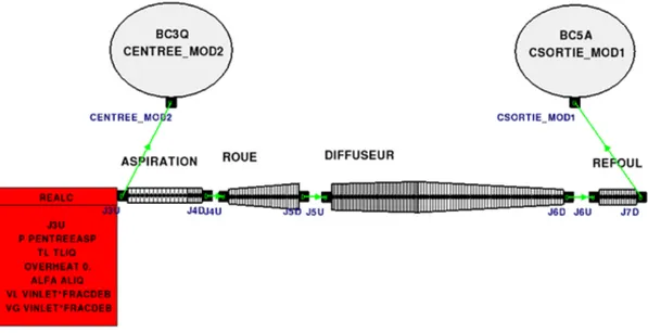
EDF, CETIM and ArianeGroup) and one academic lab (LMFL). It was decided at the end of year 2015 to implement a predictive transient, two-phase flow rotodynamic pump model in the CATHARE code and validate results at component scale (pump) and system scale (reactor) with respect to available experimental data. Flow inside parts of the pump (suction, impeller, diffuser, volute) is computed according to a one-dimensional discretization. A mean flow path has to be defined for such a modelling. Even if the subject of the 1D pump performance prediction is not new, some recent works are still investigating this field by proposing some improvements of the loss coefficients or slip factor correlations (Kara Omar et al 2017 [10], El Naggar 2013 [6], Ji et al 2010 [9]). Nevertheless most of this works are limited to steady operations and only few studies are proposing quantitative predictions of a pump during transient operations (Tanaka et Tsukamoto 1999 [12], Dazin et al 2007 [3]). Moreover, according to the authors’ knowledge, most of the performance prediction models used in hydraulic system software are limited to the prediction of the pump operating in the normal pump quadrant, by the use of inlet/outlet veloc-ity triangles based tools. The originalveloc-ity of the present project is to build a real 1D model -the mean streamline in the different parts of the pumps is meshed- able to predict the performance of mixed and radial flow pumps in purely liquid or gas/liquid, and four quadrant operations. An example of the CATHARE-3 1D modelling applied to the DERAP pump is shown on figure 1 below. Four one-dimensional elements are defined to represent the pump: the suction, the impeller, the diffuser and volute (together) and the discharge pipe.
Figure 1: CATHARE-3 1D modelling of the DERAP pump
The global strategy of the CATHARE-3 1D pump model developpement project and the first pump-scale validation results have been presented ealier (Matteo et al 2018 [11]). The ability of the model to predict head and torque as a function of time during a 1-second pump fast start-up has been proved when imposing rotational speed evolution and flow rate as a boundary condition. In the present paper, not only pump behaviour validation is desired but also system response. For this reason, a whole loop is modelled and the rotational speed time evolution is the only imposed boundary condition. Flow rate and pressure boundary conditions are no more needed because loop elements interact with each other. The loop support of this study is the
DERAP test bench installed at LMFL. It was the support of several previous studies (Dazin et al 2007 [3], Duplaa 2008 [4], Duplaa et al 2010 [5]).
Development support: the CATHARE-3 code
CATHARE-3 is a french two-phase flow modular system code. It is owned and developped since 1979 by CEA and its partners EDF, Framatome and IRSN. See [1] for more details on the code development and validation strategy. One-dimensional (1D), three-dimensional (3D) or point (0D) hydraulic elements can be associated together to represent a whole facility. They respectively correspond to one or three directions allowed for the fluid, and to components where fluid velocity is negligible such as capacities. Thermal and hydraulic submodules (as warming walls, valves, pumps, turbines...etc) can be added to the main hydraulic elements to respectively take into account thermal transfer, flow limitation, pressure rise or pressure drop. Six local and instantaneous balance equations (mass, momentum and energy for each phase) make possible liquid and gas representation for transient calculations. Mechanical and thermal disequilibrium between phases can thus be represented [7]. Phase average imposes the use of physical closure laws in the balance equations system [2].
1 DERAP PUMP DESCRIPTION AND 1D MODELLING 1.1 Description of the DERAP centrifugal pump
The DERAP pump has been set in Mechanical Laboratory of Lille (LMFL) to study the pump behaviour in cavitating and non-cavitating operating conditions during fast startups. Single-phase and two-Single-phase cavitating characteristics are available in the first operating quadrant for this pump [4]. Here only single-phase characteristics will be used to validate 1D-pump model results. DERAP impeller is shown on figures 2 and 3 below. After modelling DERAP using the CATHARE-3 1D-pump developed model, the pump data deck shown on figure 1 is obtained. Diffuser and volute also have been modelled in this study.
Figure 2: DERAP impeller picture and
geo-metric specifications. Figure 3: DERAP impeller scheme. More information on DERAP pump geometric data is available in Duplaa [5]. DERAP specific speed value is 12.3 according to the common european definition of specific speed called Nsq (defined in [8]). DERAP nominal point is QN = 23m3/h, HN = 50m and NN =
2900rpm.
1.2 Improvement of the diffuser and volute modelling
Remaining discrepancies observable in a previous study (Matteo et al 2018 [11]) have been supressed by improving the modelling of the pump stator. Previously, the impeller was the only part entirely modelled: centrifugal acceleration and relative velocity were calculated inside the
impeller, desadaptation and recirculation losses were taken into account. But the flow was ideally redressed directly when entering the diffuser, what was a first simple approach. In the present study, the diffuser part is entirely modelled taking into account the two components of the velocity in the diffuser and volute parts. Additionally to the better representation of the velocity profile, diffusion losses are modelled in the volute part. Flow is progressively redressed in the volute part, in order to get a one-component axial velocity at the end of the volute.
1.3 Prediction of DERAP performance curves
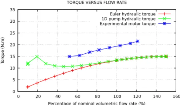
Head and torque performance curves can be observed on the following figures (4 and 5). Predicted head performance is quasi-superimposed with the experimental performance excepted at low flow rate. This discrepancy can be explained by the way the deviation model is applied. Indeed, currently the deviated angle is calculated at nominal flow rate and applied for every flow rate. A reflexion is currently carried out to chose to improve the slip factor in a larger operating range. 0 20 40 60 80 100 120 0 20 40 60 80 100 120 140 160 Manometric head (m)
Percentage of nominal volumetric flow rate (%) MANOMETRIC HEAD VERSUS FLOW RATE
Euler head 1D pump head Experimental head
Figure 4: Head performance curve.
0 5 10 15 20 25 30 35 0 20 40 60 80 100 120 140 160 Tor que (N.m)
Percentage of nominal volumetric flow rate (%) TORQUE VERSUS FLOW RATE
Euler hydraulic torque 1D pump hydraulic torque Experimental motor torque
Figure 5: Torque performance curve. The experimental torque plotted on figure 5 is a mechanical torque, which includes the disk and mechanical friction torques. It cannot directly be compared to the hydraulic torque predicted by the 1D pump model. But, the friction torque can be assumed to be independent on flow rate, and for this reason it can be said that a good agreement exists between experimental and computed torque (slopes of both curves are very close, in particular around nominal flow rate).
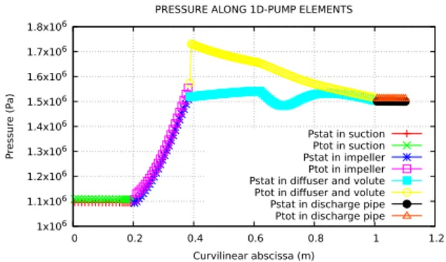
One of the biggest interest of the CATHARE-3 1D pump model is that profiles inside pump elements can be obtained during the computation. As an example, figures 6 and 7 below have been drawn at nominal rotational speed and flow rate. Figure 6 represents the total and static pressures along the pump elements. Figure 7 represents the velocity along the pump elements.
1x10⁶ 1.1x10⁶ 1.2x10⁶ 1.3x10⁶ 1.4x10⁶ 1.5x10⁶ 1.6x10⁶ 1.7x10⁶ 1.8x10⁶ 0 0.2 0.4 0.6 0.8 1 1.2 P ressur e (P a) Curvilinear abscissa (m) PRESSURE ALONG 1D-PUMP ELEMENTS
Pstat in suction Ptot in suction Pstat in impeller Ptot in impeller Pstat in diffuser and volute Ptot in diffuser and volute Pstat in discharge pipe Ptot in discharge pipe
Figure 6: Static and total pressures profile along the flow path at nominal operating point. 4 6 8 10 12 14 16 18 20 22 0 0.2 0.4 0.6 0.8 1 1.2 V elocity (m/s) Curvilinear abscissa (m) VELOCITY ALONG 1D-PUMP ELEMENTS
Absolute velocity in suction Relative velocity in impeller Absolute velocity in diffuser and volute Absolute velocity in discharge pipe
Figure 7: Velocity profile along the flow path at nominal operating point.
It has to be noted that inside the rotating part (impeller) the velocity is the relative one, whereas it is the absolute one in the fixed parts (with only one axial component in the suction part, and with two components (axial and tangential) in the diffuser and volute parts). High velocities in the diffuser part can be observed, which cause friction losses. The flow direction evolution can be seen in the diffuser and volute. The absolute flow angle α (calculated towards the tangential direction) is gradually increased from its value at the diffuser outlet toπ2 according to a cubic fitting. The bump observable on both the pressure and velocity profiles in the volute part can be explained by this fitting. To validate or improve this profiles, more local experimen-tal data or computations results are necessary. CFD computations could be used following an up-scaling method to validate this type of 1D results.
2 CATHARE-3 DERAP facility modelling 2.1 Whole facility description
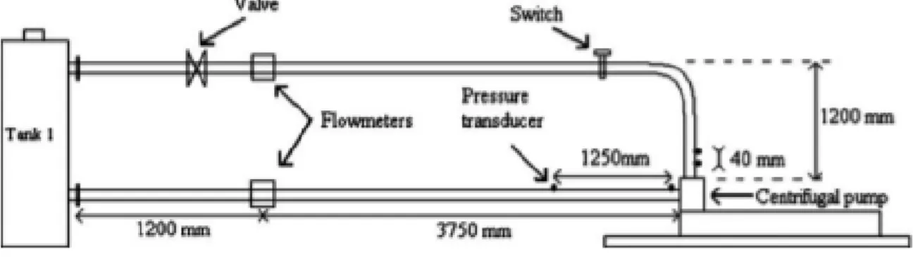
The DERAP test rig set at the Mechanical Laboratory of Lille (LMFL) has been used by Duplaa [5] to experiment cavitation during fast startup transients. The test rig installed in the LMFL allows for two configurations : a closed circuit with the suction and delivery pipes connected to a single tank, and an open one with two separate tanks, whose pressures can be set independently. A valve is used to switch from one to the other. The closed configuration has been used for the experiments represented here. For the DERAP closed configuration loop, two pipes are used to link the pump suction and delivery to a single tank, whose pressure can be set by the user (see figure 8). A control valve is located on the delivery pipe, its purpose is to control the steady state flow rate. Two pressure transducers are used on the test rig : one 50mm upstream of the impeller on the suction pipe and another 100mm downstream on the delivery pipe.
Figure 8: Scheme of the test rig
Before two-phase tests, Duplaa conducted a one-phase fast startup, while imposing a suffi-cient pressure in the tank to avoid cavitation. This test is modelled with the CATHARE-3 code and results are presented in the following sections.
2.2 CATHARE-3 modelling
The CATHARE-3 modelling of the circuit was done using 1D and 0D elements. Compared to the figure 1, the suction and delivery elements have been extented in order to represent the whole pipes of the DERAP loop. A singular pressure loss coefficient is used to take into account loss due to the elbow on the delivery pipe. The regular losses in the pipes are calculated by CATHARE, and a good precision is obtained when roughness of the pipe material is provided by the user (here stainless steel).
Figure 9: CATHARE modelling of the complete circuit
The tank is a large fluid capacity with several connections, thus a 0D element has been used to represent it. Its two junctions are linked to the suction and delivery pipes (figure 9).
The same geometry as the one used in the component scale data deck (figure 1) is used for the impeller, diffuser and volute parts. Only the orientation of elements has been adapted to
well connect the whole circuit. In particular, the volute outlet height is respected compared to the experimental setup. These 1D elements are placed on the bottom right of figure 9.
2.3 Fast startup transient
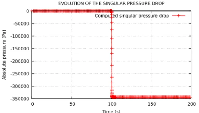
The experimental procedure followed by Duplaa consisted in first starting slowly the pump and to adjust the flow control valve in order to obtain the desired flow rate. Then, the pump was stopped and after stabilization of the circuit, the fast startup was launched. In the computation, the flow control valve is modelled by a singular pressure drop which is adjusted to obtain the desired flow rate at the end of the transient. The experimental position of the flow control valve in the circuit is respected. Pressure drop caused by the singular element is shown on figure 10 below. -350000 -300000 -250000 -200000 -150000 -100000 -50000 0 0 50 100 150 200 Absolute pr essur e (P a) Time (s)
EVOLUTION OF THE SINGULAR PRESSURE DROP Computed singular pressure drop
Figure 10: Singular pressure drop evolution.
0 0.0001 0.0002 0.0003 0.0004 0.0005 0.0006 0.0007 0 50 100 150 200 Flowrate (kg/s) Time (s)
EVOLUTION OF GAS FLOW AT THE TANK VALVE Computed gas flowrate
Figure 11: Valve flow evolution. Similarly to what was done in the experiment, pressure at the top of the tank is regulated at 2.8 bar. The tank is full of liquid except at the very top where there is a free surface with compressed air above it. The pressure regulation is done the same way in the calculation using a gas injection/extraction valve. Injected gas is non-condensable air gas. Gas flow evolution at the pressure regulation valve is shown on figure 11. It can be seen that some air is injected at the top of the tank in the first 20 seconds in order to rise pressure to 2.8 bar.
In the first 100 seconds of the CATHARE computation, the circuit is stabilized with a pump almost stopped. This means that a residual rotational speed is defined in order to initialize the circuit with a little flow rate of 3.10−5m3/s (0.47% of nominal flow rate). 0% flow rate
computation is to avoid for numerical reasons.
The fast startup begins at 100 s and finishes at 101.5 s. Rotational speed evolution is imposed by a time dependent law. It follows the experimental one as shown on figure 12. The aim of this validation work is to predict the flow rate, head (pressure difference) and torque evolutions and to compare it to available experimental data.
0 50 100 150 200 250 300 350 400 100 100.2 100.4 100.6 100.8 101 101.2 101.4 R
otational speed (rad/s)
Time (s) ROTATIONAL SPEED EVOLUTION
Imposed rotational speed Experimental rotational speed
Figure 12: Rotational speed evolution (im-posed by a time dependent law).
0 0.001 0.002 0.003 0.004 0.005 0.006 0.007 0.008 100 100.2 100.4 100.6 100.8 101 101.2 101.4 Flow rate (m3/s) Time (s) FLOW RATE EVOLUTION
Computed flow rate Experimental flow rate
Figure 13: Flow rate evolution (predicted by the model and compared to experi-ment).
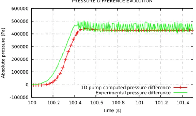
Predicted flow rate and pressure difference evolutions are respectively presented on fig-ures 13 and 14. A good agreement is obtained when comparing predictions of the model to experimental data. The differences between the flow rate evolutions are certainly due to the measurement uncertainty as the flow evolution is very difficult to measure during a fast startup. Torque evolution is shown on figure 15. Observable discrepencies are mostly due to the fact that the plotted experimental torque is a mechanical torque measured on the shaft, whereas the computed torque is an hydraulic torque. The experimental torque contains friction torques in addition to the hydraulic torque (the same observation has been previously made on torque performance curves of figure 5).
-100000 0 100000 200000 300000 400000 500000 600000 100 100.2 100.4 100.6 100.8 101 101.2 101.4 Absolute pr essur e (P a) Time (s)
PRESSURE DIFFERENCE EVOLUTION
1D pump computed pressure difference Experimental pressure difference
Figure 14: Pressure difference evolution (pre-dicted by the model and compared to experi-ment). -0.03 -0.02 -0.01 0 0.01 0.02 0.03 0.04 100 100.2 100.4 100.6 100.8 101 101.2 101.4 Tor que coe ffi cient (-) Time (s) TORQUE EVOLUTION
1D pump computed hydraulic torque Experimental mechanical torque
Figure 15: Torque evolution (predicted by the model and compared to experi-ment).
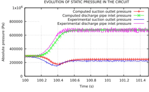
With the complete loop modelling, pressures can be analyzed at different points in the cir-cuit. On figure 16 computed and experimental suction outlet pressure and discharge pipe inlet pressure are shown.
It can be seen that pressure is rising at the discharge pipe inlet (this corresponds to the pump pressure rise) unlike it is droping at the suction pipe outlet (because of inertial effects in the pipe). These two pressure evolutions are well predicted by the model by comparison to experimental pressure evolutions from Duplaa et al 2010 [5]. 0 200000 400000 600000 800000 1x10⁶ 100 100.2 100.4 100.6 100.8 101 101.2 101.4 Absolute pr essur e (P a) Time (s)
EVOLUTION OF STATIC PRESSURE IN THE CIRCUIT Computed suction outlet pressure Computed discharge pipe inlet pressure Experimental suction outlet pressure Experimental discharge pipe inlet pressure
Figure 16: Pressure evolutions (pre-dicted by the model and compared to ex-periment).
CONCLUSIONS
This paper presents a whole pump loop modelled with the CATHARE-3 thermal-hydraulic code. First, the 1D modelling of DERAP pump ”alone” is presented and predicted performances are compared to experimental ones. A good agreement is obtained. Then, the complete system scale modelling is presented and results obtained during a 1-second fast startup transient are analyzed. With the complete loop modelling, it is possible to follow the evolution of several physical quantities of interest such as the gas flow injected or extracted at the top of the tank for pressure regulation for example, or pressures at different points of the circuit, etc. This is done in the present study. This first validation at loop system scale is a step bringing to analysis of reactor system scale response during hypothetical accidental transients of interest (pump seizure, pump stop on inertia, pump restart, cavitation occuring in working pumps, inverse flow rate and/or rotation speed...). This paper presents one-phase computations, but two-phase computations have started recently and the next step is to validate the fast startup transient with cavitation occuring in the pump (see Duplaa 2010 for experimental description of the two-phase tests).
ACKNOWLEDGEMENTS
Thanks to the LMFL universitary lab and Framatome, ArianeGroup, CETIM and EDF in-dustrial companies who support the project by providing data, funding or knowledge.
References
[1] F. Barre and M. Bernard. The CATHARE code strategy and assessment. Nuclear Engi-neering and Design, 124:257–284, 1990.
[2] D. Bestion. The physical closure laws in the CATHARE code. Nuclear Engineering and Design, 124:229–245, 1990.
[3] A. Dazin, G. Caignaert, and G. Bois. Transient behavior of turbomachineries: applications to radial flow pump startups. Journal of Fluids Engineering, 129, 2007.
[4] S. Duplaa. Etude exp´erimentale du fonctionnement cavitant d’une pompe lors de s´equences de d´emarrage rapide. PhD thesis, Arts et M´etiers ParisTech, 2008.
[5] S. Duplaa, O. Coutier-Delgosha, A. Dazin, O. Roussette, G. Bois, and G. Caignaert. Ex-perimental study of a cavitating centrifugal pump during fast startups. Journal of Fluids Engineering, 132, 2010.
[6] M. A. El-Naggar. A one-dimensional flow analysis for the prediction of centrifugal pump performance characteristics. International Journal of Rotating Machinery, 2013, 2013. [7] B. Faydide and J.C. Rousseau. Two-phase flow modeling with thermal and mechanical
non equilibrium. In European Two Phase Flow Group Meeting, Glasgow UK, 1980. [8] J. F. G¨ulich. Centrifugal Pumps. Springer, 2014.
[9] C. Ji, J. Zou, X.D. Ruan, P. Dario, and X. Fu. A new correlation for slip factor in radial and mixed-flow impellers. In Proc. IMechE, volume 225, 2010.
[10] A. Kara-Omar, A. Khaldi, and A. Ladouani. Prediction of centrifugal pump performance using energy loss analysis. Australian Journal of Mechanical Engineering, 15:3:210–221, 2017.
[11] L. Matteo, A. Dazin, and N. Tauveron. Development and validation of a one-dimensional transient rotodynamic pump model at component scale. In IAHR, Kyoto Japan, 2018. [12] T. Tanaka and H. Tsukamoto. Transient behaviour of a cavitating centrifugal pump at rapid
change in operating conditions-part 3: Classifications of transient phenomena. Journal of Fluids Engineering, 121:857–865, 1999.