The Gender Wage Gap and Sample Selection via Risk Attitudes

HAL Id: halshs-00965520

https://halshs.archives-ouvertes.fr/halshs-00965520v2

HAL is a multi-disciplinary open access archive for the deposit and dissemination of sci-entific research documents, whether they are pub-lished or not. The documents may come from teaching and research institutions in France or

L’archive ouverte pluridisciplinaire HAL, est destinée au dépôt et à la diffusion de documents scientifiques de niveau recherche, publiés ou non, émanant des établissements d’enseignement et de recherche français ou étrangers, des laboratoires

The Gender Wage Gap and Sample Selection via Risk

Attitudes

Seeun Jung

To cite this version:

Seeun Jung. The Gender Wage Gap and Sample Selection via Risk Attitudes. 2014. �halshs-00965520v2�

WORKING PAPER N° 2014

– 10

The Gender Wage Gap and Sample

Selection via Risk Attitudes

Seeun Jung

JEL Codes: J24; J31; D81; C52

Keywords: Occupational Choice; Gender Wage Gap; Risk Preference; Selection Bias

P

S

E

48, BD JOURDAN – E.N.S. – 75014 PARIS

TÉL. : 33(0) 1 43 13 63 00 – FAX : 33 (0) 1 43 13 63 10

The Gender Wage Gap and Sample

Selection via Risk Attitudes

Seeun Jung

Abstract

This paper investigates a new way to estimate the gender wage gap with the introduction of individual risk attitudes using representative Korean data. We es-timate the wage gap with correction for the selection bias, which latter results in the overestimation of this wage gap. Female workers are more risk averse. They hence prefer working in the public sector, where wages are generally lower than in the private sector. It goes on to explain the reduced gender wage gap by develop-ing an appropriate sample-selection model, with wage decompositions corrected for selectivity. Self-selection based on risk attitudes therefore explains, in part, what is popularly perceived as gender discrimination.

JEL Classification: J24; J31; D81; C52

Keywords: Occupational Choice; Gender Wage Gap; Risk Preference; Selection Bias

∗_{Paris School of Economics and Sciences Po Paris, [email protected]}

†_{The author is grateful for comments by Andrew E. Clark, Luc Arrondel, Fabrice Etil´e, Thomas}

Dohmen, Ronald Oaxaca, Chung Choe, seminar participants at ISER & GCOE Behavioral Economics Joint Seminar of Osaka University, at CEPS/INSTEAD seminar in Luxembourg, at PRESAGE/OFCE seminar, the conference of EALE 2011 Cyprus, and the EEA meeting 2013 Gothenberg. The financial support of CEPREMAP is gratefully acknowledged.

1

Introduction

Many factors can affect an individual’s decisions about economic issues. In human-capital theory, risk is involved when students make education decisions, such as weighing random future income against an additional year of education. In the labor market, some people choose to endure longer periods of unemployment in order to obtain better wages and working conditions, while some prefer to exit unemployment sooner despite lower wages. Others prefer lower wages and safer public-sector pension and social security plans to higher wages and riskier private-sector pension and social security plans.

A number of reasons may underlie these choices. First, markets might not clear such that firms do not offer the same wage profiles to identical workers. Second, there could be individual heterogeneity in the decision-making process. Even when all observable factors are controlled for - such as gender, age, wealth, region, etc. - there are still significant differences in outcomes. This suggests the presence of unobservable factors behind individual heterogeneity and firm behavior.

Since, Adam Smith argued that the wage could be determined by different

character-istics of jobs (such as risk) in his book ‘Wealth of Nations’ in (Smith (1776)), the theory

of compensating wage differentials have been widely studied. Murphy et al. (1987) and

Moore (1995) show that job sectors with higher unemployment and greater risk tend to

have higher wages. Hence, job-sorting decisions may well vary with individuals’ attitudes

to risk. More recent work such as Hartog et al. (2003) also shows that jobs with greater

risk are paid higher wages, contributing to the theory of compensating wage differentials. Workers who are more willing to accept a certain number of dollars for a given increase in risk are more likely to choose to work in riskier jobs than those who are less inclined to make a trade-off between wages and risk. While job-sector choice is sensitive to differences in risk attitudes, it is a priori also strongly correlated with education decisions.

Measuring attitudes to risk is, however, a delicate task, and there have been various attempts to find the right kind of subjective self-reported variables that accurately reflect

risk aversion. Feinberg (1977) and Hersch and Viscusi (1990) study the use of seatbelts

and smoking behavior. Ekelund et al.(2005) use a psychometric variable measuring harm

avoidance as an indicator of risk attitudes. They find that agents with a higher harm-avoidance score (i.e. less risk averse) are more likely to become self-employed, which is considered riskier than being employed as a wage earner. In an experimental study,

Dohmen et al.(2005) show that measures of subjective risk attitudes, such as self-reported

risk aversion and lottery questions, provide a valid predictor of actual risk behavior.

Dohmen and Falk (2011) build upon these results and use self-reported risk aversion in

the German Socioeconomic Panel to see whether risk preferences explain how individuals

are sorted into occupations with different earnings variation. Furthermore, Luechinger

et al.(2007) andPfeifer(2011) analyze selection in public-sector employment, andGrund

and Sliwka (2006) and Cornelissen et al. (2011) study pay-for-performance schemes. All

conclude that risk-averse workers have a greater preference for non-competitive working

environments. Pissarides (1974) presents a theoretical model explaining that risk-averse

workers have lower reservation wages. This relationship is demonstrated empirically

by Pannenberg (2007). Similarly, Goerke and Pannenberg (2008) show that there is a

negative relationship between risk aversion and union membership.

Given that job sorting matters in terms of the position actually held in the labor market, there is good reason to wonder whether the job-sorting decision interacts with the gender disparity observed on the labor market. Although the gender bias in education has been reduced and the education gap between men and women has narrowed in recent

decades (Arnot et al. (1999)), there is still concern over the considerable wage gap and

other kinds of gender-based discrimination on the labor market. In a move to explain

these findings, Croson and Gneezy (2009) and Bertrand (2011) argue that women may

be more risk averse and less competitive than men. More interestingly for our question,

Gneezy et al. (2003), Niederle and Vesterlund (2007) and Croson and Gneezy (2009) all

suggest that differences in risk attitudes might partly explain the gender gap in

et al. (2007) show that job-sector selection and wages are correlated with risk attitudes. Here, then, lies our centre of interest. The gender wage gap is still an interesting issue for labor economists and policymakers. In many countries, even developed countries like Sweden where gender rights are believed to be the most equal in the world, gender wage differentials are often observed. Labor economists analyze this phenomenon and define the

gender wage gap as “discrimination” if it occurs for equally-productive workers (Becker

(1993)). A huge body of literature has been produced in this field to examine the wage

gap and discrimination following the seminal paper of Oaxaca(1973). The raw wage gap

is decomposed into two parts: one explained by human capital and endowments, and the other unexplained, which is often deemed to be discrimination. Empirical estimations of

wages with human capital commonly use a Mincerian wage equation (Mincer (1974)), in

which the logarithm of wage is regressed on observable socio-demographic variables such as gender, schooling, age, etc. In this model, however, concerns may arise in the event of selection issues or omitted variable bias: what would the level of wages have been in the absence of discrimination? A number of contributions have attempted to correct

this selection bias, mainly based on the selection of labor-market participation (Neuman

and Oaxaca(2004)). We here instead consider sector selection (followed by participation

selection) to decompose the gender wage gap, considering selection via individual risk attitudes.

This paper shows how female workers appear to choose to work in the lower-paid public sector, and how individual risk attitudes can play a role in this decision-making process. It goes on to explain the reduced gender wage gap by developing an appropriate sample-selection model. The remainder of the paper is organized as follows. Section 2 introduces the simple conceptual framework behind the idea, and then presents the analytical framework with the data description in Section 3. Section 4 shows the empirical results obtained from testing the impact of risk aversion on job sorting and the gender wage gap with corrected selection bias. Last, Section 5 concludes.

2

Conceptual Framework

Public-sector jobs are often considered to be safer in terms of their associated benefits, job stability and security. However, they also pay less than private-sector jobs, where workers obtain a wage premium for taking risks such as higher job separation rates and fewer or lower-quality benefits. For this reason, we might expect risk-averse workers to prefer public-sector stability over private-sector wage volatility and a greater probability of unemployment in the private sector. In addition, female workers are more sorted into the public rather than the private sector, which might be explained by gender difference in risk attitudes. In this paper, we define the risk in the private sector as the existence of a severe job separation rate, which is higher in the private sector than in the public sector.

This section introduces some simple occupational self-sorting concepts in terms of attitudes towards risk.

2.1

Risk-Averse Workers’ Preference for the Public Sector

We assume that individuals can have two types of risk attitudes: risk averse and less risk averse (or risk neutral, risk loving). We then assume two types of firms. First, there is the competitive firm (private sector), where the job-separation rate is higher (and job security is lower, since workers are more likely to be fired). Second, there is the non-competitive firm (public sector) with a lower job separation rate. We assume that the competitive firms offer a wage premium p > 0 to offset the job-security risk. We say that workers

in non-competitive firms receive a risk-free wage wpu while workers in competitive firms

obtain the risk-free wage plus a risk premium p (i.e. wpr = wpu+ p). The assumption

here is that the job-separation rate is higher for competitive than non-competitive firms

rpu < rpr. In the extreme case, we could set rpu = 0 with no risk of being fired and

rpr = r > 0. Taking the basic CRRA utility function with different risk aversion factors

ρ: u(c) = c1−ρ

> ρRN (less risk-averse individuals)). If a worker is fired, s/he receives a basic government

subsidy of b, with b < wpu < wpr. If we take the non-competitive firm wage as wpu = w,

the competitive firm wage would be w + p and the basic subsidy b could also be rewritten

as w − p′ _{for a given positive value p}′_{. Provided that the risk premium is greater than}

r

1−rp

′_{, expected earnings are higher in competitive than non-competitive firms. We now}

turn to expected utility. Workers with greater risk aversion would choose to work in non-competitive firms even though the wage is lower from the CRRA utility function. Given the same wage premium and job-separation ratio, expected utility varies with the level of ρ. We are, here, interested in finding the condition that satisfies the following:

→ EU (wpu) > EU (wpr) for risk-averse workers with ρRA

→ EU (wpu) < EU (wpr) for less risk-averse workers with ρRN

This is the case when the following condition holds:

r ∈ [ (w + p)

1−ρRA_{− w}1−ρRA

(w + p)1−ρRA− (w − p′)1−ρRA,

(w + p)1−ρRN _{− w}1−ρRN

(w + p)1−ρRN − (w − p′)1−ρRN]

Given this range of job-separation rates for competitive firms r, risk-averse workers are better off choosing the non-competitive firms with lower wages. In addition, the market clears within this range, so that both risk-averse and less risk-averse workers maximize their utility. If the ratio is greater than the upper (less than the lower) bound, both workers choose to work in non-competitive (competitive) firms with lower wages (higher

risks). This range of job-separation rates broadens as the difference between ρRA and

ρRN grows, p′ grows (unemployment income falls), and the wage premium p shrinks.

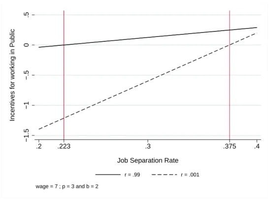
Figure 1 shows the results of the simulated incentives to work in the public sector, where these incentives are simply the difference between the expected utilities of working in the public and private sectors. This incentive rises with risk aversion for any concave utility function. More risk-averse workers (with a parameter close to 1) prefer the public sector. Analogously, Figure 2 shows the simulated incentives to work in the public sector by the job-separation rate. The solid line represents a risk-averse worker (with ρ = 0.99), while the dashed line corresponds to a risk-neutral worker (ρ = 0.001). When the

job-−.6

−.4

−.2

0

.2

Incentives for working in Public

0 .2 .4 .6 .8 1

Risk Aversion

wage = 7 ; p = 3; b = 2 and r = .3

Figure 1: Incentives to Work in the Public Sector by Risk Aversion

−1.5

−1

−.5

0

.5

Incentives for working in Public

.2 .223 .3 .375 .4

Job Separation Rate

r = .99 r = .001

wage = 7 ; p = 3 and b = 2

separation rate lies inside the brackets which satisfy the condition above1

, we see that the risk-averse worker has positive incentives to work in the public sector, while the risk-neutral worker is better off working in the private sector.

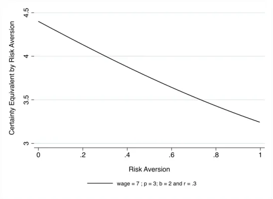
Then, we could also calculate for the certainty equivalent for bearing job-separation risks in the private sector:

CE = [r(w + p)1−ρ_{+ (1 − r)(b)}1−ρ_]1−ρ1

Figure 3 presents the simulation result for the certainty equivalent over risk aversion. Working in the private sector is taking a risk to be fired and earn an unemployment subsidy b with a probability r (job-separation rate) in our case. The certainty equivalent is decreasing as risk aversion increases given a certain job-separation rate (0.3). Figure 4 shows the changes in the certainty equivalent when the risk increases (i.e. job-separation rate increases) for two different types of individual in terms of risk aversion (for example, men vs women). It shows that when there is any sort of risk, the certainty equivalent of more risk-averse individuals is lower than that of less risk-averse individuals. Also, when the risk is certain (i.e. when r is either 0 or 1), there is no difference in the certainty equivalent. Overall, we could infer that if women are more risk averse, then their certainty equivalent for choosing to work in the private sector is lower than men’s. Therefore, they would accept the public-job offers at lower wage in which men would reject. This explains why women are more sorted into the public sector.

2.2

Gender Difference in Expected Returns

Imagine again that there are two types of firms. One pays higher wages, but the atmo-sphere is highly competitive and the job is not secure. The other firm is relatively relaxed and the job is more secure, but pays a lower wage than the competitive firm. Looking at the competitive type of firm, we show below that this firm pays male workers higher

1_{In our calculation using the parameter we use for the simulation, the range of the job-separation}

3 3.5 4 4.5 C e rt a in ty Eq u iva le n t b y R isk A ve rsi o n 0 .2 .4 .6 .8 1 Risk Aversion wage = 7 ; p = 3; b = 2 and r = .3

Figure 3: Certainty Equivalent for Bearing Risk of Job Separation in the Private Sector by

Risk Aversion 2 4 6 8 10 C e rt a in ty Eq u iva le n t b y Jo b Se p a ra ti o n R a te 0 .2 .4 .6 .8 1

Job Separation Rate

r = .3 r = .8 wage = 7 ; p = 3 and b = 2

Figure 4: Certainty Equivalent for Bearing Risk of Job Separation in the Private Sector by Job

wages than female workers.

There is less guarantee that a woman will return to the job in the competitive firm after child bearing than to a job in the public sector, where maternity leave is better-accepted. Assuming that women’s quitting rates from competitive firms are higher than men’s due to their child bearing, following which the competitive firms may not guarantee keeping

their job positions open (i.e. qf > qm), the expected return for a given period after hiring

by gender with productivity a and hiring cost of c, a > c > 0 (both identical by gender)

in the competitive firms is the following: Πf = a(1 − qf) − cqf < Πm = a(1 − qm) − cqm.

Therefore, it makes sense for the competitive firm to prefer to hire male workers (i.e. male workers’ probability of being hired is greater than that of female workers). More

risk-averse workers set their reservation wages lower in order to be hired (Pissarides

(1974)), whereas less risk-averse workers have a lower probability of being hired albeit

keeping their reservation wage higher. This leads more risk-averse female workers to accept lower wage offers in the competitive firms. Therefore, among female workers in the competitive firm, risk-averse workers earn lower wages. This idea ties in with the

“statistical discrimination”2

literature, in that there are different wage profiles emanating from the demand side (firms).

3

Analytical Framework

Bearing in mind the two scenarios in the previous section, we now set up an analytical framework in order to test them empirically. A number of pieces of work have investigated whether the gender gap in risk-taking preferences and competitiveness is significantly

dif-ferent and even innate. Apicella et al.(2008) show that risk-taking in an investment game

with potential real monetary pay-offs correlates positively with salivary testosterone levels

and facial masculinity. More recently,Buser(2011) finds that women are less competitive

both when taking contraceptives that contain progesterone and estrogen and during the

2_{Statistical discrimination is a theory of inequality between demographic groups based on stereotypes}

phase of the menstrual cycle when the secretion of these hormones is particularly high.

Hormone studies aside, Sutter and Rutzler (2010) examine the compensation choices of

1,000 Austrian children and teenagers aged 3 to 18, and find that the gender gap in competitiveness is already present by age 3.

Here, we note that the working environment in the public sector and the private sector is far different. While in the private sector, the working condition is rather competitive and risky, public jobs offer rather stable and secure types of working enviornment. There-fore, the wage equation should be differently estimated by sectors. As the choice of sectors are not random but determined by risk aversion causing endogeneity issues, we should control for the selectivity. In this section, we will discuss about selection correction and the modified gender wage gap.

3.1

Selection

The concern often raised with the Mincerian wage equation is that the employment sector is wage-endogenous. There are omitted variables which could influence both wages, gender, and sector selection. If we do not control for this selection, the results from the wage equations will not only be biased, but also the coefficients will be inconsistent. Here we use a risk-attitude variable to correct for selection and obtain adjusted estimates of the gender wage gap, as risk aversion which is correlated with gender, could determine

workers’ employment sector choices.3

3.1.1 Switching Regression Model

Roy (1951), Maddala (1983), and Nakosteen and Zimmer (1980) propose a model to

address the earnings of migrants and non-migrants (the move stay model). In our paper, we apply their method to deal with self-selection. We estimate the earnings for

public-3_{Regarding the exclusion restriction, Korean labor market wages are quite rigid once people are}

employed and are often not negotiable on entering the market. Therefore, risk aversion can be assumed to affect wages only in terms of sector selection. However, we will appeal to polychotomous choice sample-selection models to discuss this issue in the following section.

sector workers and private-sector workers separately.

wpub,i = Xpub,i′ βpub+ ǫpub,i : P ublic W age Equation

wpri,i= Xpri,i′ βpri+ ǫpri,i : P rivate W age Equation

The sector-selection function is:

P ub∗

i = δRAi+ Zi′γ + ui : Sector Choice

P ubi = 1 if P ub∗i > 0 : In P ublic

where P ub∗

i is a latent variable such that if P ub∗i > 0 then P ubi takes the value of 1 (choice

of the public sector), otherwise P ubi takes the value of 0 (choice of the private sector);

RAi is the variable that captures individual risk attitudes (hereafter risk aversion) and

Zi is a vector of characteristics influencing the employment-sector decision.

We use direct Direct Maximum-Likelihood estimation (Lokshin and Sajaia(2006)) for

the two-stage approach in this paper. The log-likelihood for this model is, then,

ln L =X

i

(P ubi[ln{Φ(ηpub,i)} + ln{φ(ǫǫpub,i/σpub)/σpub}]+

(1 − P ubi)[ln{1 − Φ(ηpri,i)} + ln{φ(ǫǫpri,i/σpri)/σpri}])

where Φ is a cumulative normal distribution function, φ is a normal density distribution function, and ηji = δRAi+ Zi′γ + ρjǫji/σj q 1 − ρ2 j , j = pub, pri

where ρpub is the correlation coefficient between ǫpub,i and ui, ρpri is the correlation

coef-ficient between ǫpri,i and ui, σ2u is a variance of the error term in the selection

equa-tion, and σ2

pub and σ

2

pri are the variances of the error terms in the wage equations.

σǫpri,u = Cov(ǫpri,i, ui).

If we take the condition P ubi = 1 (i.e. workers in the public sector), the earning

equation for workers in the public sector is as follows:

E(wpub,i|xpub,i, P ubi = 1) = Xpub,i′ βpub+ E(ǫpub,i|ui > −δRAi− Zi′γ)

= X′

pub,iβpub+ σpubρpub

φ(−δRAi− Zi′γ)

1 − Φ(−δRAi− Zi′γ)

= X′

pub,iβpub+ σpubρpub

φ(δRAi+ Zi′γ)

Φ(δRAi+ Zi′γ)

The correlation coefficient determines the effect of selection on the conditional income of

workers in the public sector. If ρpub is significantly different from zero, we cannot ignore

the unobservable characteristics that could affect both selection and earnings. The wage equation for workers in the private sector can similarly be written as:

E(wpri,i|xpri,i, P ubi = 0) = Xpri,i′ βpri+ E(ǫpri,i|ui ≤ −δRAi− Zi′γ)

= Xi′βpri+ σpriρpri[−

φ(−δRAi− Zi′γ)

Φ(−δRAi− Zi′γ)

]

= Xpri,i′ βpri− σpriρpri

φ(δRAi+ Zi′γ)

1 − Φ(δRAi+ Zi′γ)

Furthermore, we can calculate the hypothetical expected log wage (i.e. public-sector workers’ expected wages if they worked in the private sector and private-sector workers’ expected wages if they worked in the public sector).

E(wpub,i|xpri,i, P ubi = 0) = Xpub,i′ βpub− σpubρpub

φ(δRAi+ Zi′γ)

1 − Φ(δRAi+ Zi′γ)

E(wpri,i|xpub,i, P ubi = 1) = Xpri,i′ βpri+ σpriρpri

φ(δRAi+ Zi′γ)

3.1.2 Polychotomous Choice Sample Selection Model

We now consider the case where people choose from five alternatives when they enter the labor market; (1) employment in the public sector, (2) employment in the private sector, (3) self-employed, (4) unemployed, and (5) inactive. This factors in the possibility that risk aversion could affect wages via one more channel: the reservation wage associated

with entering employment.4

The selection correction models based on the multinomial

logit have been developed byLee(1983),Dubin and McFadden(1984), and more recently

Bourguignon et al.(2007). Consider the following polychotomous choice model with five

categories:

wj = Xj′βj + ρjuj

s∗j = δRAj+ Zjγj+ vj

where j = 1, 2, 3, 4, 5 and uj ∼ N (0, 1). If we assume that vj is i.i.d with a Gumbel

distribution, the probability of individual i choosing j is

P (sij = 1) = exp(ηij) 1 +P5_k=1exp(ηik) if j > 1 or = 1 1 +P5_k=1exp(ηik) if j = 1 where ηij = maxk=1,2,3,4,5 k6=j(s∗k− vj).

The bias-corrected wage equation by Dubin and McFadden (1984) is then

w1 = X1′β1+ σ X j=2,3,4,5 ρj( Pjln(Pj) 1 − Pj + ln(P1)) + ǫj

where Pj is the probabilities to choose j and (σρ) is the coefficient term for the

poly-chotomous correction of the selectivity bias; ǫj is an orthogonal error parameter towards

the rest of terms, which allows us to use directly OLS in the estimation.

4

3.2

Wage Gap

3.2.1 Pooled

ln wij = αjF emaleij + Xi′βj+ uij : P ooled W age Equation

ln wif j = Xi′βf j+ uif j : F emale W age Equation

ln wimj = Xi′βmj + uimj : M ale W age Equation

The wage can be estimated by a general Mincerian wage equation. We estimate the log of wages of individual i at a sector j where j could be either public, private, self-employment, unemployment, and inactive, with a dummy variable of being F emale and X, a set of control variables of socio-demographic information such as years of schooling, years of experience, the experience squared, the number of weekly working hours, being regular

worker, the number of children, health status5

, and dummies for sectors and regions. The wage equation could be estimated with the pooled sample or separately by gender in each

sector. The gender gap in the j sector would be the coefficient for being female, ‘αj’.

Then we can also look at the Oaxaca-Blinder type wage gap decomposition (Oaxaca

(1973), Blinder (1973), Oaxaca and Ransom (1994), Oaxaca and Ransom (1999), and

Fortin (2008)). ln Wmj − ln Wf j = (X′m− X′f)dβmj | {z } Endowment + X′ f(dβmj − cβf j) | {z } Discrimination

3.2.2 Gender Wage Gap with Selection

With the selection correction as discussed in the previous section, we can correct the wage and then estimate the unbiased wage gap.

ln wij = φjF emaleij + Xi′λj + θjhj + ǫij : P ooled W age Equation

5_{Health status is measured by 1-5 Likert scale by asking ‘How do you define your health status}

compared to the last year?’. Health is possibly correlated with the performance which will affect the wage.

ln wif j = Xi′λf j+ θf jhf j+ ǫif j : F emale W age Equation

ln wimj = Xi′λmj + θmjhmj + ǫimj : M ale W age Equation

with θjhj as selection terms estimated through various selection methods we discussed in

the previous section. Then, the corrected gender gap in the pooled sample in the j sector

would be ‘φj’.

Then, the corrected decomposition suggested byNeuman and Oaxaca(2004) andYun

(2007) would be: ln Wmj − ln Wf j = (X′m− X′f)dλmj | {z } Endowment + X′ f(dλmj − cλf j) | {z } Discrimination + (θmjhmj− θf jhf j) | {z } Selectivity

The unbiased wage gap could be estimated by correcting the log wages with selection terms:

ln Wmj − ln Wf j− (θmjhmj − θf jhf j) = (X′m− X′f)dλmj + X′f(dλmj − cλf j)

This equation will be estimated via the Switching Regression (Nakosteen and Zimmer

(1980) andLokshin and Sajaia(2006)) and the Polychotomous Selection Model suggested

byDubin and McFadden (1984) and Bourguignon et al. (2007).

3.2.3 Identification

We use risk aversion as a key variable which determines in which sector an individual would like to work, in order to identify the impact of selection and to correct the wage. As discussed in the previous section, risk aversion is a determinant when an individual choose in which sector he prefers to work. In this paper, we assume that risk aversion does not directly affect the wage to satisfy the exclusion restriction. Although one may argue

that risk aversion can be correlated with workers’ productivity (Jung and Houngbedji

wage after controlling for the selection step. We can infer that the impact of risk aversion on the selection step is larger than that on the wage. In addition to risk aversion, we use another determinant variable which is father’s education. Family background can also determine the job-sector selection and it does not directly affect the wage. One concern is that our variable of interest, risk aversion, can also be influenced by family background, and hence, it might offset the impact of risk aversion. However, we could use father’s

education as a proxy to reveal some part of risk aversion6

. Therefore, we will keep these two variables in order to support the selection step more concretely. In the first step, we calculate the corrected wage gap using the selection terms, and then we estimate the corrected wage gap taking into account the additional terms of selectivity, which would give the gender wage gap with the correction of self-selection.

4

Data and Results

4.1

Data

This paper uses data from Korea where the gender gap is still an important labor-market issue. Even though Korea’s economy has grown remarkably over the past few decades, its gender wage gap remains the largest among member countries of the Organization for Economic Co-operation and Development (OECD). Data from the OECD’s 2009 Annual Report show that male workers in Korea are paid 40 percent more than their female counterparts. This is the widest gender wage gap of the 30 OECD member economies, being over twice the OECD average of 18.8 percent.

Our data comes from the Korean Labor & Income Panel Study published by the Korean Labor Research Institute. This survey was first launched in 1998 and has now more than 10 waves, being carried out once a year. It covers 5,000 households and their members (11,453 individuals in all) who currently live in Korea. Sample weights ensure

6_{Risk aversion is found to be correlated with parents’ background (Dohmen et al. (2005), Dohmen}

the representativeness of the survey. These panel data are interesting in that they contain questions on risk attitudes and many different elements of job and life satisfaction. For some part of this paper where the wage equations are estimated, we restrict the sample to 4,208 individuals in the one wave (2007) in which the risk questions are available, and also only consider individuals who are currently employed as wage earners in order to deal with labor-market sector selection. In the Korean sample, the occupational shares for the 11,453 individuals are shown in Table 1.

The participation rate in Korea is low in comparison to the OECD average. For example, Table 1: Occupation Share

Full Sample Men Women

Obs Rate Obs Rate Obs Rate

Inactive 5,239 45.7% 1,663 30% 3576 60.5% Active 6,214 54.3% 3,883 70% 2,331 39.5% Unemployment 319 5.1% 163 4.2% 156 6.7% Self-Employment 1,665 26.8% 1,145 29.5% 520 22.3% Public Workers 1,129 26.7% 597 23.2% 532 32.1% Private Workers 3,101 73.3% 1,978 76.8% 1,123 67.9 % Total 11,453 5,546 5,907

in Japan, the male participation rate is 84.8% in 2007, while in Korea it is 70%. Female participation rate is remarkably much lower in Korea. It is 62% in Japan, 65% in France, and 60% in an average OECD country, whereas in Korea it is less than a half of the population. Indeed, the Korean labor market is quite distorted in terms of gender view. The unemployment rate is calculated as 5% which is higher than in Japan (4.3%), but lower than the OECD average (6.2%) or in France (8.9%), for example. In our sample, 319 unemployed workers are observed, within which 84% were working in the private sector. This reassures that indeed the job-separation rate in the private sector is much higher than in the public sector as discussed in the previous section.

Table 2 displays descriptive statistics by education attainments and gender. Overall, the male participation rate into the labor force (73%) is almost double the female partic-ipation rate (42.1%), and also the female unemployment rate (6.3%) is a lot higher than

Table 2: Descriptive Statistics by Education and Gender

Participation Unemployment Public Self-Employment Rate Rate Among Wage Earners Among Active Workers

Men Women Men Women Men Women Men Women

Secondary 70.1% 36.5% 4.3% 6.6% 21.5% 34% 35% 24.7%

Tertiary 76.9% 55.4% 3.7% 5.8% 24.8% 29.7% 19.9% 15.1%

All 73% 42.1% 4% 6.3% 23.2% 32.1% 28.3% 20.9%

the male unemployment rate (4%). Among wage earners, the share of public workers in the female sample is higher than that in the male sample, while the share of self-employment is a lot higher in the male sample than in the female sample among active workers. These differences tend to reduce when we look at the high-educated sample. More high-educated women are active in the labor force, and the gender participation gap into the public sector is reduced. Also, high-educated individuals tend to choose to be wage earners, rather than self-employed among active workers.

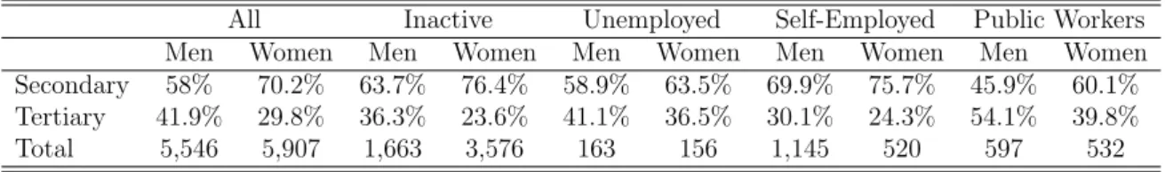
Table 3: Educational Distribution among Inactive, Unemployed, Self-Employed, and Public Workers

All Inactive Unemployed Self-Employed Public Workers

Men Women Men Women Men Women Men Women Men Women

Secondary 58% 70.2% 63.7% 76.4% 58.9% 63.5% 69.9% 75.7% 45.9% 60.1%

Tertiary 41.9% 29.8% 36.3% 23.6% 41.1% 36.5% 30.1% 24.3% 54.1% 39.8%

Total 5,546 5,907 1,663 3,576 163 156 1,145 520 597 532

Table 3 presents the educational attainments among different occupations. There is a significant difference in terms of educational attainments between gender. A bigger share (70%) of woman are low-educated whereas male education attainment bewteen low- and high-education in general is rather even. Among inactive individuals, a large share is low-educated.

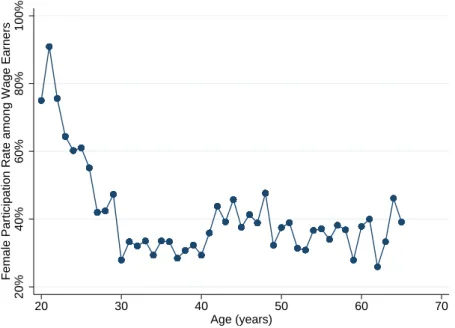
Figure 5 shows the percentage of women among wage earners in different cohorts. In Korea, women tend to enter the labor market earlier than men, since men have to serve two years of national service before entering the labor market. Women’s labor-market participation drops sharply however by the age of 30. This is often the age at which they get married.

20%

40%

60%

80%

100%

Female Participation Rate among Wage Earners

20 30 40 50 60 70

Age (years)

Figure 5: Female Participation

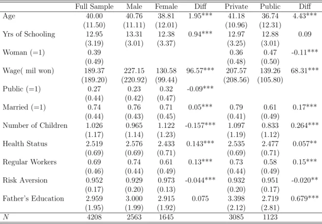
Now, we retain wage earners only (sample size of 4,208) for the switching regression model in order to look at the selection between the public and private sectors. The full sample is then used for the polychotomous selection model when estimating sector selection including the labor-market participation decision. For individual risk attitudes, we construct a measure from the answers to five lottery-type questions. Table 4 presents the summary statistics on wage earners. The proportion of female workers in the wage-earning segment of the Korean labor market is about 40%. We can first look at the gender wage differential. On average, women have lower wages (KRW130.61 million

monthly),7

fewer years of schooling (12.39 years)8

, more anxiety about their health9

, more children, less marriage, and are younger (age 39) than men (KRW227.57 million, 13.31 years education, age 41). Also less women have regular (tenured) contract at work. These characteristics of women are similar to those of public workers, except for the number of children. This lower wage could be the result of both gender discrimination

7_{1 U.S. dollar is approximately 1,100 Korean Won.}

8_{However, the difference in schooling is not much different when we restrict the sample to wage earners.}

When we look at the difference using the full sample in Table 1, there is a large educational-attainments difference between gender.

9_{Health status is measure in 1-5 Likert scale, asking ‘How do you think your health status compare}

Table 4: Summary Statistics

Full Sample Male Female Diff Private Public Diff

Age 40.00 40.76 38.81 1.95*** 41.18 36.74 4.43*** (11.50) (11.11) (12.01) (10.96) (12.31) Yrs of Schooling 12.95 13.31 12.38 0.94*** 12.97 12.88 0.09 (3.19) (3.01) (3.37) (3.25) (3.01) Woman (=1) 0.39 0.36 0.47 -0.11*** (0.49) (0.48) (0.50)

Wage( mil won) 189.37 227.15 130.58 96.57*** 207.57 139.26 68.31*** (189.20) (220.92) (99.44) (208.56) (105.80) Public (=1) 0.27 0.23 0.32 -0.09*** (0.44) (0.42) (0.47) Married (=1) 0.74 0.76 0.71 0.05*** 0.79 0.61 0.17*** (0.44) (0.43) (0.45) (0.41) (0.49) Number of Children 1.026 0.965 1.122 -0.157*** 1.097 0.833 0.264*** (1.17) (1.14) (1.23) (1.19) (1.12) Health Status 2.519 2.576 2.433 0.143*** 2.535 2.477 0.057** (0.69) (0.69) (0.71) (0.69) (0.71) Regular Workers 0.69 0.74 0.61 0.13*** 0.73 0.58 0.15*** (0.46) (0.44) (0.49) (0.44) (0.49) Risk Aversion 0.952 0.929 0.973 -0.044*** 0.932 0.951 -0.020** (0.17) (0.20) (0.13) (0.20) (0.17) Father’s Education 2.959 3.000 2.915 0.075 3.398 2.719 0.679*** (1.95) (1.99) (1.92) (2.12) (2.81) N 4208 2563 1645 3085 1123

Notes. Standard errors in parentheses *: p < 0.10, ** : p < 0.05, *** : p < 0.01

and female workers’ characteristics, such as less education and a higher proportion of women in the public sector (47% of public-sector workers are women as opposed to 36% in the private sector), where wages are generally lower (KRW207 million in the private sector and KRW140 million in the public sector). Public workers tend to be less confident with their health compared to private workers.

Figures 6 - 14 display the wage distribution of wage earners between gender. Women always earn lower wage than men. However, the gap can be reduced in higher education.

In addition, public-sector workers’ risk aversion10

is higher on average than it is for workers in the private sector. Women are also found to be more risk averse. While there is no such difference in father’s education between gender, we found that between sectors, father’s education is big and significantly different. The higher educated a father is, the

0 .2 .4 .6 .8 D e n si ty 2 4 6 8 10

Log of Monthly Income

Men Women

kernel = epanechnikov, bandwidth = 0.0961

Figure 6: Wage Distribution, Full

0 .2 .4 .6 .8 1 D e n si ty 2 4 6 8 10

Log of Monthly Income

Men Women

kernel = epanechnikov, bandwidth = 0.1011

Figure 7: Wage Distribution, Secondary Ed-ucation 0 .2 .4 .6 .8 D e n si ty 2 4 6 8

Log of Monthly Income

Men Women

kernel = epanechnikov, bandwidth = 0.1204

Figure 8: Wage Distribution, Tertiary Edu-cation

0 .2 .4 .6 .8 1 D e n sit y 2 4 6 8

Log of Monthly Income

Men Women

kernel = epanechnikov, bandwidth = 0.1288

Figure 9: Wage Distribution, Pub-lic 0 .2 .4 .6 .8 1 D e n sit y 2 3 4 5 6

Log of Monthly Income

Men Women

kernel = epanechnikov, bandwidth = 0.1417

Figure 10: Wage Distribution, Pub-lic, Secondary Education

0 .2 .4 .6 .8 1 D e n sit y 2 4 6 8

Log of Monthly Income

Men Women

kernel = epanechnikov, bandwidth = 0.1358

Figure 11: Wage Distribution, Pub-lic, Tertiary Education

0 .2 .4 .6 .8 1 D e n sit y 2 4 6 8

Log of Monthly Income

Men Women

kernel = epanechnikov, bandwidth = 0.1288

Figure 12: Wage Distribution, Pri-vate 0 .2 .4 .6 .8 1 D e n si ty 2 3 4 5 6

Log of Monthly Income

Men Women

kernel = epanechnikov, bandwidth = 0.1417

Figure 13: Wage Distribution, Pri-vate, Secondary Education

0 .2 .4 .6 .8 1 D e n si ty 2 4 6 8

Log of Monthly Income

Men Women

kernel = epanechnikov, bandwidth = 0.1358

Figure 14: Wage Distribution, Pri-vate, Tertiary Education

more they would be found in the private sector. That is because more educated fathers may influence individuals to bear some risks in order to get higher wages or simply to be more risk-seeking, as discussed in the previous section. Therefore, father’s education can be used as an input factor to determine individual risk aversion. We now describe how risk aversion is measured in our data.

4.2

Measuring Risk Aversion

The Korean Labor & Income Panel Study recently added in a number of pilot questions on individual risk attitudes. We use the 2007 wave, which contains lottery questions that we can use to summarize individual risk-taking attitudes. Each individual is asked whether they would accept the given lottery or take KRW100,000 (USD 82) in cash, or whether they are indifferent between the two. The details of the three questions that we use for this study are shown below:

Name Lottery characteristics Expected Value Indifferent LottoM 1/2: KRW200,000, 1/2: KRW0 KRW100,000 Risk Neutral

LottoL 3/5: KRW200,000, 2/5: KRW0 KRW120,000 Risk Averse LottoH 2/5: KRW200,000, 3/5: KRW0 KRW80,000 Risk Seeking

Here, the three choices - denoted LottoM, LottoL, and LottoH - differ in their degree of riskiness. Taking LottoM as the baseline, LottoL is less risky than LottoM while LottoH is riskier. By comparing the cash KRW100,000 with the expected value of lotteries, we could identify the individual to be risk neutral, risk averse, or risk seeking if she is indifferent between the lottery and the cash.

We use the answers to these three questions to construct a risk-aversion variable, which may well explain a part of individual heterogeneity. We follow the method first introduced

by Barsky et al. (1997), categorising individuals into several groups which differ in risk

aversion. The mechanism of categorising individuals into different risk-attidude groups is presented in Figure 15.

LottoM LottoL Risk-Averse Category= 5 Cash/In_differen t Risk-Averse Category= 4 Lotto Ca_sh Risk-Averse Category= 3 Indifferent LottoH Risk-Averse Category= 2 Cash Risk-Averse Category= 1 Lotto/In different Lott o

Figure 15: Categorising Risk-Attitude Groups by Choices of Lotteries

Starting with LottoM in the first stage, we can make the following three categories: (1) choosing the cash, (2) being indifferent, and (3) choosing the lottery. As being indifferent in this lottery corresponds to risk neutrality, we can sort individuals who prefer the cash into the averse group, while those who prefer the lottery are sorted into the risk-seeking group. If their choice of LottoM is either the lottery or the cash, then we can subdivide those individuals into two groups. If the choice of LottoM is the cash, we consider LottoL which is less risky. If the choice of LottoM is the lottery, we consider LottoH which is riskier. In LottoL, being ‘indifferent’ also means ‘risk averse’ as the expected value is less than KRW100,000, because the distance between the expected value and KRW100,000 could be seen as a risk premium from choosing the lottery. Similarly, being indifferent in LottoH means ‘risk seeking’. Based on these answers, we create 5 categories in ascending order of risk-averse level. We divide each risk-averse categorical value by 5 in order to get a risk aversion variable that is ranged between 0 and 1.

.9

.92

.94

.96

.98

Average Risk Aversion

20 30 40 50 60

Age groupd by 10 years

Women Men Figure 16: RA by Gender .92 .94 .96 .98 1

Average Risk Aversion

20 30 40 50 60

Age grouped by 10 years Public Private Figure 17: RA by Sector .9 .92 .94 .96 .98 1

Average Risk Aversion

20 30 40 50 60

Age groupd by 10 years

Men in Public Men in Private

Figure 18: RA by Sector, Men

.95

.96

.97

.98

.99

Average Risk Aversion

20 30 40 50 60

Age grouped by 10 years

Women in Public Women in Private

Table 5: Risk-Aversion Measures Mean SE Obs Full Sample 0.929 0.21 11453 Male 0.929 0.21 5546 Female 0.973 0.13 5907 Diff Male-Female -0.044*** 0.013 Private 0.932 0.20 1123 Public 0.951 0.17 3085 Diff Private-Public -0.019** 0.008 Inactive or SE 0.960 0.16 7245

Diff Employed-Non emp -0.023*** 0.003

Edu > 12yrs 0.935 0.20 7362 Edu ≤ 12yrs 0.961 0.16 4091 Diff -0.026** 0.003 Age < 45 0.935 0.20 6419 Age ≥ 45 0.973 0.13 5034 Diff -0.038*** 0.003 Not married 0.936 0.19 2931 Married 0.957 0.16 8522 Diff -0.021*** 0.004 Notes. *: p < 0.10, ** : p < 0.05, *** : p < 0.01

Table 5 shows risk aversion in the different sub-samples: by gender, job sector, educa-tion, age, and marital status. Female workers are more risk averse than male workers and workers in the public sector are more risk averse than those in the private sector. Em-ployed workers (both in the public and the private) tend to be less risk averse than those who are in other status (self-employed or inactive). In addition, highly-educated workers tend to be less risk averse than workers who have a high school diploma. Older workers (aged over 45) are more risk averse, while marital status is also significantly linked with risk aversion. We do indeed find a gender difference in attitude towards risk, which is the basis for the work we carry out here. Figure 16 shows the relationship between risk aversion and age by gender. Women have a tendency to be more risk averse than men at all ages. This figure also shows a positive slope, suggesting an age effect on risk aversion. Both for men and women, workers in the public sector have higher risk aversion than in the private sector (Figure 17). This trend is clearer in male sample (Figure 18). This is because in the labor market, aged women are rather influenced by domestic issues such

as taking care of their children. Therefore, over a certain age (40 years old), risk aversion is no longer a determinant for the sector selection as other factors have a larger impact (Figure 19). It could also be that aged women are at disadvantage at work and hence they do not have as many choices as male workers have. Overall, risk aversion varies across gender and sectors, which gives a right reason to use the selection analyses.

4.3

Results

Table 6 presents the results of pairwise correlation matrix for the variables in which we are interested. The main risk-aversion variable is significantly correlated with wage, gender, employment, sector selection, education, being married, health, and father’s education. Being female, working in the public sector, and being married are all positively correlated with risk aversion, while the correlation with wage, employment, education, and health status are negative. The signs and significance are in line with human-capital theory and the literature on risk. Wages are lower for women and in the public sector, and women are more often found in the public sector. In addition, we note that father’s education is negatively correlated with risk aversion, which is supporting our identification and

the literature (Dohmen et al. (2005), Dohmen et al. (2012), and Hryshko et al. (2011)).

These correlations are the starting point of our analyses. Tables 7, 8, and 9 show the Table 6: Pairwise Correlation of Variables

RA LW W E P E M H F Risk Aversion 1.000 Log Wage -0.103* 1.000 Woman (=1) 0.127* -0.410* 1.000 Employed -0.065* 0.000* -0.191* 1.000 In Public 0.042* -0.256* 0.099* 0.000* 1.000 Education -0.112* 0.441* -0.213* 0.238* -0.014 1.000 Married 0.054* 0.121* 0.097* -0.009 -0.177* -0.294* 1.000 Health -0.061* 0.163* -0.116* 0.138* -0.037* 0.339* -0.218* 1.000 Father Edu -0.023* 0.036* -0.021* 0.101* -0.145* 0.027* 0.004 0.007 1.000 Notes. *: p < 0.10

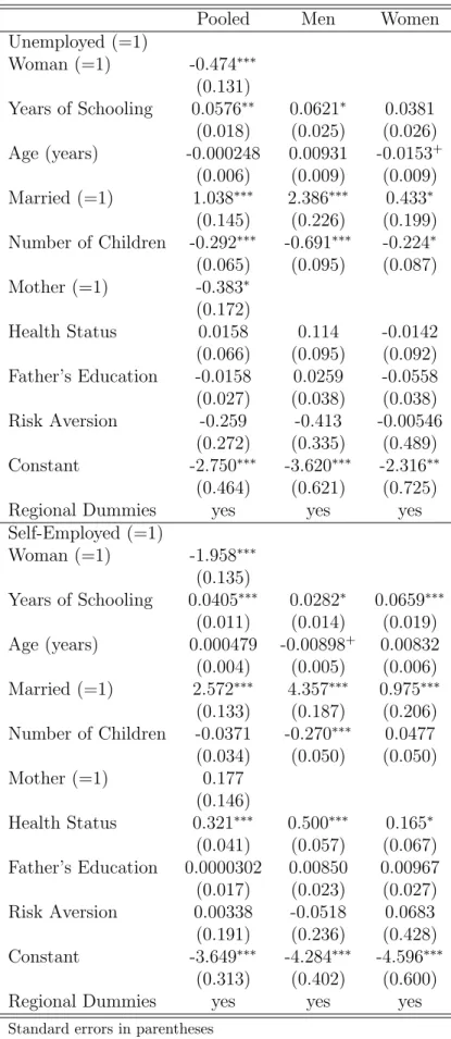
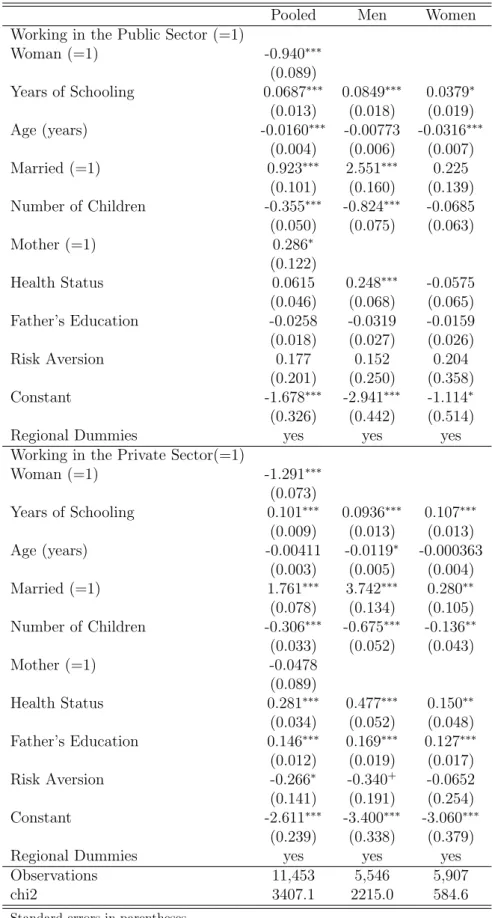
selection steps, we consider being woman, age, marital status, the number of children, being mother, and health status as the main explanatory variables for sector choices. We also included regional dummies to control differences in regional labor-market conditions. Risk aversion and father’s education are used as excluded variables for the selection methods. Table 7 estimates the binary choice in order to investigate what factors explain the decision to work in the public sector; the binary dependent variable is public-sector employment (=1) among wage earners only. The subjects who choose to work in the public sector are as expected more risk averse. Father’s education is negatively correlated with the selection into the public sector. This father’s education variable may offset the impact of risk aversion as risk aversion can be influenced by family background as we discussed in the identification section. Also, being mother is definitely a determinant to make women to work in the public sector. Years of schooling, age, health and marital status are all negatively correlated with working in the public sector. Tables 8 and 9 show the Multinomial Logit Model results for: (1) being inactive as the reference point; (2) being unemployed; (3) being self-employed (Table 8); (4) working in the public sector; and (5) working in the private sector (Table 9). Risk aversion is negatively correlated with the unemployment (not significant) and not correlated with being self-employed. Also public workers are more risk averse without significance. However, it becomes a significant determinant of working in the private sector: the more risk-seeking the individual is, the more likely they choose to work in the private sector.

Overall, mothers tend to choose (or to be pushed to choose) the public sector.

Edu-cation is positively correlated with selection into the private sector. Health11

is positively and significantly correlated with working in the private sector; workers who are confident in their health may prefer to work in the private sector. Our variable of interest, risk aversion is, indeed, negatively correlated with the private-sector choice: workers with greater risk aversion are more often found in the public sector. Father’s education is positively (negatively) correlated with working in the private (public) sector (although

Table 7: Selection Step: Binary Choice between Public and Private

Pooled Men Women

Public (=1) Woman (=1) -0.0177 (0.062) Years of Schooling -0.0422∗∗∗ _-0.0258∗ _-0.0692∗∗∗ (0.008) (0.011) (0.014) Age (years) -0.0260∗∗∗ _-0.0207∗∗∗ _-0.0353∗∗∗ (0.004) (0.005) (0.005) Married (=1) -0.367∗∗∗ _-0.542∗∗∗ _0.0210 (0.061) (0.075) (0.096) Number of Children 0.0338 0.0561 0.0682 (0.033) (0.043) (0.048) Mother (=1) 0.315∗∗∗ (0.083) Health Status -0.125∗∗∗ _-0.115∗∗ _-0.129∗∗ (0.031) (0.042) (0.048) Father’s Education -0.105∗∗∗ _-0.116∗∗∗ _-0.0920∗∗∗ (0.011) (0.015) (0.017) Risk Aversion 0.218+ 0.236+ 0.153 (0.117) (0.136) (0.237) Constant 1.537∗∗∗ _1.205∗∗∗ _2.101∗∗∗ (0.235) (0.297) (0.393)

Regional Dummies yes yes yes

Observations 4230 2575 1655

chi2 357.0 234.2 99.38

Standard errors in parentheses

+

Table 8: Selection Step: Multiple Choice among Inactive, Unemployed, Self-Employed, Public and Private

Pooled Men Women

Unemployed (=1) Woman (=1) -0.474∗∗∗ (0.131) Years of Schooling 0.0576∗∗ _0.0621∗ _0.0381 (0.018) (0.025) (0.026) Age (years) -0.000248 0.00931 -0.0153+ (0.006) (0.009) (0.009) Married (=1) 1.038∗∗∗ _2.386∗∗∗ _0.433∗ (0.145) (0.226) (0.199) Number of Children -0.292∗∗∗ _-0.691∗∗∗ _-0.224∗ (0.065) (0.095) (0.087) Mother (=1) -0.383∗ (0.172) Health Status 0.0158 0.114 -0.0142 (0.066) (0.095) (0.092) Father’s Education -0.0158 0.0259 -0.0558 (0.027) (0.038) (0.038) Risk Aversion -0.259 -0.413 -0.00546 (0.272) (0.335) (0.489) Constant -2.750∗∗∗ _-3.620∗∗∗ _-2.316∗∗ (0.464) (0.621) (0.725)

Regional Dummies yes yes yes

Self-Employed (=1) Woman (=1) -1.958∗∗∗ (0.135) Years of Schooling 0.0405∗∗∗ _0.0282∗ _0.0659∗∗∗ (0.011) (0.014) (0.019) Age (years) 0.000479 -0.00898+ _0.00832 (0.004) (0.005) (0.006) Married (=1) 2.572∗∗∗ _4.357∗∗∗ _0.975∗∗∗ (0.133) (0.187) (0.206) Number of Children -0.0371 -0.270∗∗∗ _0.0477 (0.034) (0.050) (0.050) Mother (=1) 0.177 (0.146) Health Status 0.321∗∗∗ _0.500∗∗∗ _0.165∗ (0.041) (0.057) (0.067) Father’s Education 0.0000302 0.00850 0.00967 (0.017) (0.023) (0.027) Risk Aversion 0.00338 -0.0518 0.0683 (0.191) (0.236) (0.428) Constant -3.649∗∗∗ _-4.284∗∗∗ _-4.596∗∗∗ (0.313) (0.402) (0.600)

Regional Dummies yes yes yes

Table 9: Selection Step: Multiple Choice among Inactive, Unemployed, Self-Employed, Public and Private-Continued

Pooled Men Women

Working in the Public Sector (=1)

Woman (=1) -0.940∗∗∗ (0.089) Years of Schooling 0.0687∗∗∗ _0.0849∗∗∗ _0.0379∗ (0.013) (0.018) (0.019) Age (years) -0.0160∗∗∗ _{-0.00773 -0.0316}∗∗∗ (0.004) (0.006) (0.007) Married (=1) 0.923∗∗∗ _2.551∗∗∗ _0.225 (0.101) (0.160) (0.139) Number of Children -0.355∗∗∗ _-0.824∗∗∗ _-0.0685 (0.050) (0.075) (0.063) Mother (=1) 0.286∗ (0.122) Health Status 0.0615 0.248∗∗∗ _-0.0575 (0.046) (0.068) (0.065) Father’s Education -0.0258 -0.0319 -0.0159 (0.018) (0.027) (0.026) Risk Aversion 0.177 0.152 0.204 (0.201) (0.250) (0.358) Constant -1.678∗∗∗ _-2.941∗∗∗ _-1.114∗ (0.326) (0.442) (0.514)

Regional Dummies yes yes yes

Working in the Private Sector(=1)

Woman (=1) -1.291∗∗∗ (0.073) Years of Schooling 0.101∗∗∗ _0.0936∗∗∗ _0.107∗∗∗ (0.009) (0.013) (0.013) Age (years) -0.00411 -0.0119∗ _-0.000363 (0.003) (0.005) (0.004) Married (=1) 1.761∗∗∗ _3.742∗∗∗ _0.280∗∗ (0.078) (0.134) (0.105) Number of Children -0.306∗∗∗ _-0.675∗∗∗ _-0.136∗∗ (0.033) (0.052) (0.043) Mother (=1) -0.0478 (0.089) Health Status 0.281∗∗∗ _0.477∗∗∗ _0.150∗∗ (0.034) (0.052) (0.048) Father’s Education 0.146∗∗∗ _0.169∗∗∗ _0.127∗∗∗ (0.012) (0.019) (0.017) Risk Aversion -0.266∗ _-0.340+ -0.0652 (0.141) (0.191) (0.254) Constant -2.611∗∗∗ _-3.400∗∗∗ _-3.060∗∗∗ (0.239) (0.338) (0.379)

Regional Dummies yes yes yes

Observations 11,453 5,546 5,907

chi2 3407.1 2215.0 584.6

Standard errors in parentheses

+

the correlation is not significant for the public sector), as it is negatively correlated with risk aversion. In addition, we compare the gender difference. While risk aversion and father’s education are more important for men’s decision in the sectoral choice, it is being mother and the number of children that are more important for women’s decision. In other words, the impacts derived from the innate preference (risk aversion and father’s education in our case) has a weaker influence on the sectoral choice for women compared to men. This could hint at a potential involuntary sorting of women or more restrictions of female working conditions due to heavy domestic work, while men could more actively choose their preferred working sector. However, the results show that the direction of the impact of risk aversion and father’s education for both groups are consistent with differences in size, which will, in turn, modify the corrected wage gap. Therefore, the selection correction reveals the differences in the gender wage gap in both sectors.

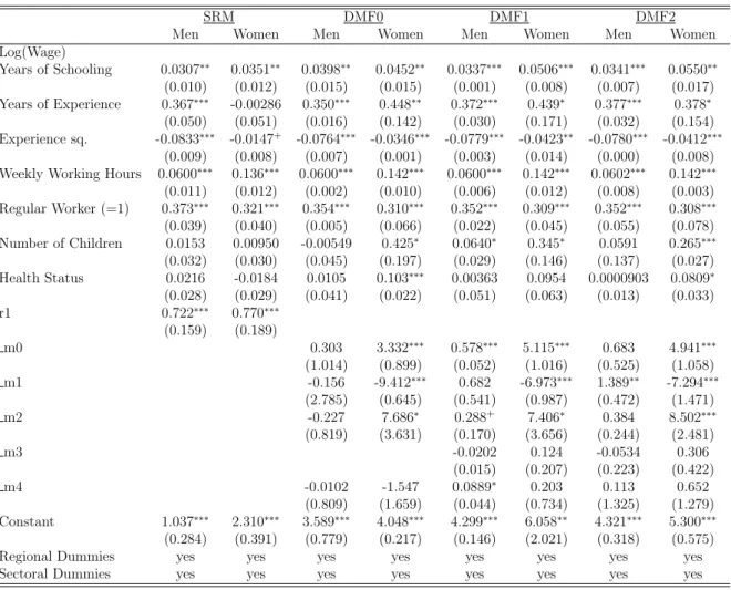
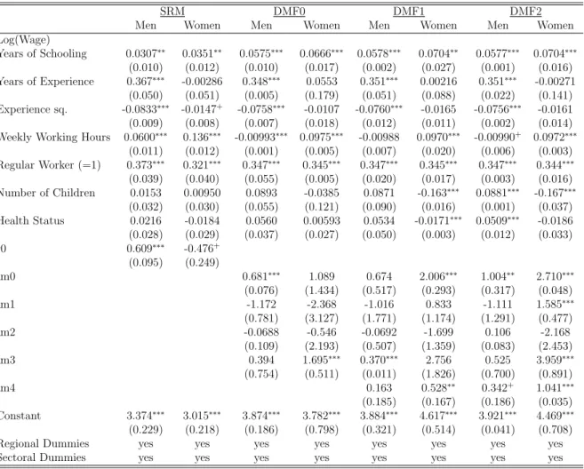
Tables 10 and 11 present the results of various men-women wage equations by sectors

using two different selection-correction methods; the Switching Regression Model (

Nakos-teen and Zimmer (1980)) (hereafter abbreviated to SRM12

) and Dubin and McFadden

(1984)’s polychotomous method (hereafter abbreviated to DMF13

). For the use of DMF,

we applied three kinds of correction: DMF0 performs the Dubin and McFadden (1984)

correction method, DMF1 performs theDubin and McFadden (1984) correction method,

waving the restriction (imposed inDubin and McFadden(1984)) that all correlation

coef-ficients sum-up to zero, and last, DMF2 performs a variant of the Dubin and McFadden

(1984) correction method suggested in Bourguignon et al. (2007). Similar to a usual

Mincerian wage equation, the schooling and experience effects are in the same direction with diffferent sizes. Also the wage increases with the number of weekly working hours and being a regular worker with tenure, allowing different sizes by sector and gender. In addition to a Mincerian wage equation, we included the control function as an additional regressor. The correlation coefficients in Tables 10 and 11 which are the correlations

12_{We use the ‘movestay’ Stata command developed by Lokshin and Sajaia (2006) to estimate the}

switching regression.

13_{We use the ‘selmlog’ Stata command developed byBourguignon et al. (2007) to estimate the}

Table 10: Men-Women Wage Equation in the Public Sector

SRM DMF0 DMF1 DMF2

Men Women Men Women Men Women Men Women

Log(Wage) Years of Schooling 0.0307∗∗ _0.0351∗∗ _0.0398∗∗ _0.0452∗∗ _0.0337∗∗∗ _0.0506∗∗∗ _0.0341∗∗∗ _0.0550∗∗ (0.010) (0.012) (0.015) (0.015) (0.001) (0.008) (0.007) (0.017) Years of Experience 0.367∗∗∗ _{-0.00286 0.350}∗∗∗ _0.448∗∗ _0.372∗∗∗ _0.439∗ _0.377∗∗∗ _0.378∗ (0.050) (0.051) (0.016) (0.142) (0.030) (0.171) (0.032) (0.154) Experience sq. -0.0833∗∗∗ _-0.0147+ _-0.0764∗∗∗ _-0.0346∗∗∗ _-0.0779∗∗∗ _-0.0423∗∗ _-0.0780∗∗∗ _-0.0412∗∗∗ (0.009) (0.008) (0.007) (0.001) (0.003) (0.014) (0.000) (0.008) Weekly Working Hours 0.0600∗∗∗ _0.136∗∗∗ _0.0600∗∗∗ _0.142∗∗∗ _0.0600∗∗∗ _0.142∗∗∗ _0.0602∗∗∗ _0.142∗∗∗

(0.011) (0.012) (0.002) (0.010) (0.006) (0.012) (0.008) (0.003) Regular Worker (=1) 0.373∗∗∗ _0.321∗∗∗ _0.354∗∗∗ _0.310∗∗∗ _0.352∗∗∗ _0.309∗∗∗ _0.352∗∗∗ _0.308∗∗∗ (0.039) (0.040) (0.005) (0.066) (0.022) (0.045) (0.055) (0.078) Number of Children 0.0153 0.00950 -0.00549 0.425∗ _0.0640∗ _0.345∗ _{0.0591 0.265}∗∗∗ (0.032) (0.030) (0.045) (0.197) (0.029) (0.146) (0.137) (0.027) Health Status 0.0216 -0.0184 0.0105 0.103∗∗∗ _{0.00363 0.0954 0.0000903 0.0809}∗ (0.028) (0.029) (0.041) (0.022) (0.051) (0.063) (0.013) (0.033) r1 0.722∗∗∗ _0.770∗∗∗ (0.159) (0.189) m0 0.303 3.332∗∗∗ _0.578∗∗∗ _5.115∗∗∗ _{0.683 4.941}∗∗∗ (1.014) (0.899) (0.052) (1.016) (0.525) (1.058) m1 -0.156 -9.412∗∗∗ _{0.682 -6.973}∗∗∗ _1.389∗∗ _-7.294∗∗∗ (2.785) (0.645) (0.541) (0.987) (0.472) (1.471) m2 -0.227 7.686∗ _0.288+ _7.406∗ _{0.384 8.502}∗∗∗ (0.819) (3.631) (0.170) (3.656) (0.244) (2.481) m3 -0.0202 0.124 -0.0534 0.306 (0.015) (0.207) (0.223) (0.422) m4 -0.0102 -1.547 0.0889∗ _{0.203 0.113 0.652} (0.809) (1.659) (0.044) (0.734) (1.325) (1.279) Constant 1.037∗∗∗ _2.310∗∗∗ _3.589∗∗∗ _4.048∗∗∗ _4.299∗∗∗ _6.058∗∗ _4.321∗∗∗ _5.300∗∗∗ (0.284) (0.391) (0.779) (0.217) (0.146) (2.021) (0.318) (0.575)

Regional Dummies yes yes yes yes yes yes yes yes

Sectoral Dummies yes yes yes yes yes yes yes yes

Standard errors in parentheses

+

Table 11: Men-Women Wage Equation in the Private Sector

SRM DMF0 DMF1 DMF2

Men Women Men Women Men Women Men Women

Log(Wage) Years of Schooling 0.0307∗∗ _0.0351∗∗ _0.0575∗∗∗ _0.0666∗∗∗ _0.0578∗∗∗ _0.0704∗∗ _0.0577∗∗∗ _0.0704∗∗∗ (0.010) (0.012) (0.010) (0.017) (0.002) (0.027) (0.001) (0.016) Years of Experience 0.367∗∗∗ _{-0.00286 0.348}∗∗∗ _{0.0553 0.351}∗∗∗ _{0.00216 0.351}∗∗∗ _-0.00271 (0.050) (0.051) (0.005) (0.179) (0.051) (0.088) (0.022) (0.141) Experience sq. -0.0833∗∗∗ _-0.0147+ _-0.0758∗∗∗ _{-0.0107 -0.0760}∗∗∗ _{-0.0165 -0.0756}∗∗∗ _-0.0161 (0.009) (0.008) (0.007) (0.018) (0.012) (0.011) (0.002) (0.014)

Weekly Working Hours 0.0600∗∗∗ _0.136∗∗∗ _-0.00993∗∗∗ _0.0975∗∗∗ _{-0.00988 0.0970}∗∗∗ _-0.00990+ _0.0972∗∗∗

(0.011) (0.012) (0.001) (0.005) (0.007) (0.020) (0.006) (0.003) Regular Worker (=1) 0.373∗∗∗ _0.321∗∗∗ _0.347∗∗∗ _0.345∗∗∗ _0.347∗∗∗ _0.345∗∗∗ _0.347∗∗∗ _0.344∗∗∗ (0.039) (0.040) (0.055) (0.005) (0.020) (0.017) (0.003) (0.016) Number of Children 0.0153 0.00950 0.0893 -0.0385 0.0871 -0.163∗∗∗ _0.0881∗∗∗ _-0.167∗∗∗ (0.032) (0.030) (0.055) (0.121) (0.090) (0.016) (0.001) (0.037) Health Status 0.0216 -0.0184 0.0560 0.00593 0.0534 -0.0171∗∗∗ _0.0509∗∗∗ _-0.0186 (0.028) (0.029) (0.037) (0.027) (0.050) (0.003) (0.012) (0.033) r0 0.609∗∗∗ _-0.476+ (0.095) (0.249) m0 0.681∗∗∗ _{1.089 0.674 2.006}∗∗∗ _1.004∗∗ _2.710∗∗∗ (0.076) (1.434) (0.517) (0.293) (0.317) (0.048) m1 -1.172 -2.368 -1.016 0.833 -1.111 1.585∗∗∗ (0.781) (3.127) (1.771) (1.174) (1.291) (0.477) m2 -0.0688 -0.546 -0.0692 -1.699 0.106 -2.168 (0.109) (2.193) (0.507) (1.359) (0.083) (2.453) m3 0.394 1.695∗∗∗ _0.370∗∗∗ _{2.756 0.525 3.959}∗∗∗ (0.754) (0.511) (0.011) (1.826) (0.700) (0.891) m4 0.163 0.528∗∗ _0.342+ _1.041∗∗∗ (0.185) (0.167) (0.186) (0.035) Constant 3.374∗∗∗ _3.015∗∗∗ _3.874∗∗∗ _3.782∗∗∗ _3.884∗∗∗ _4.617∗∗∗ _3.921∗∗∗ _4.469∗∗∗ (0.229) (0.218) (0.186) (0.798) (0.321) (0.514) (0.041) (0.708)

Regional Dummies yes yes yes yes yes yes yes yes

Sectoral Dummies yes yes yes yes yes yes yes yes

Standard errors in parentheses

+

between the errors of the wage equations and the errors of the selection equations can provide the direction of the average selection for men and women. For example, looking at SRM for male workers, as r1 is positive and significantly different from zero, men who intentionally choose to work in the public sector earn higher wages than a random man from the sample (or currently working in the other sector) would earn. Yet, r0 is positive and significantly different from zero (note that positive r0 indicates the negative selection in SRM). The model suggests that men who intentionally choose to work in the private sector earn lower wages than a random individual from the sample (or currently working in the other sector) would earn. In other words, those who entered the public sector if they had been placed in the private sector, they would have done better than those who actually entered the private sector. However, women in SRM are positively selected in both sector, meaning that observed wages overestimate female wage in both sectors. Now, we turn to the selectivity coefficients in DMF. For example, the selectivity coefficients related to the inactivity are positive and significant in the female-public wage equation (Table 10). In other words, female wages in the public sector are overestimated as women with worse unobserved characteristics were sorted into inactivity. The public-sector selectivity-correction coefficients in the private-public-sector wage equation ( m3 in Table 11) and the private-sector selectivity-correction coefficients in the public sector ( m4 in Table 10) are all positive (and sometimes significant), but differ in size between gender. With these different selectivity coefficients by gender, the corrected pooled wage gap will certainly be modified.

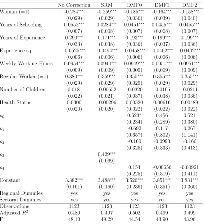
Tables 12 and 13 present the pooled wage equation by sector with various selection methods. Column (1) is a usual OLS Mincerian wage equation. In the Korean sample, female workers earn about 28.4% in the public sector and about 38.1% in the private less on average than male workers, controlling for other socio-demographic variables. Returns to education are 5.5%-7%, which is fairly standard. Being regular workers who hold tenure increases wages by 37%-38%. Female workers in the public sector are paid less (28.4%), but the gap is narrower than in the private sector (38.1%). This could

Table 12: Pooled Wage Equation with Selection Correction in the Public Sector No Correction SRM DMF0 DMF1 DMF2 Woman (=1) -0.284∗∗∗ _-0.259∗∗∗ _-0.185∗∗∗ _-0.164∗∗∗ _-0.158∗∗∗ (0.029) (0.029) (0.036) (0.039) (0.040) Years of Schooling 0.0552∗∗∗ _0.0284∗∗∗ _0.0451∗∗∗ _0.0455∗∗∗ _0.0455∗∗∗ (0.007) (0.008) (0.007) (0.008) (0.007) Years of Experience 0.290∗∗∗ _0.171∗∗∗ _0.193∗∗∗ _0.199∗∗∗ _0.199∗∗∗ (0.033) (0.038) (0.036) (0.037) (0.036) Experience sq. -0.0525∗∗∗ _-0.0494∗∗∗ _-0.0458∗∗∗ _-0.0402∗∗∗ _-0.0402∗∗∗ (0.006) (0.006) (0.006) (0.006) (0.006)

Weekly Working Hours 0.0954∗∗∗ _0.0940∗∗∗ _0.0949∗∗∗ _0.0951∗∗∗ _0.0951∗∗∗

(0.009) (0.009) (0.009) (0.009) (0.009) Regular Worker (=1) 0.380∗∗∗ _0.359∗∗∗ _0.350∗∗∗ _0.355∗∗∗ _0.355∗∗∗ (0.029) (0.029) (0.029) (0.029) (0.029) Number of Children -0.0181 -0.00652 -0.0320 -0.0165 -0.0211 (0.022) (0.021) (0.037) (0.038) (0.036) Health Status 0.0300 -0.00296 0.00520 0.00616 0.00489 (0.020) (0.020) (0.022) (0.022) (0.022) ρ0 0.523∗ 0.456 0.521 (0.234) (0.289) (0.380) ρ1 -0.692 0.117 0.267 (0.657) (0.802) (1.141) ρ2 -0.160 -0.0993 -0.166 (0.325) (0.333) (0.413) ρ3 0.429∗∗∗ (0.069) ρ4 0.154 -0.00656 -0.00921 (0.225) (0.319) (0.411) Constant 3.382∗∗∗ _3.488∗∗∗ _3.526∗∗∗ _3.851∗∗∗ _3.831∗∗∗ (0.161) (0.160) (0.236) (0.351) (0.360)

Regional Dummies yes yes yes yes yes

Sectoral Dummies yes yes yes yes yes

Observations 1123 1123 1123 1123 1123

Adjusted R2 _{0.480 0.497 0.502 0.499 0.499}

F 48.10 49.29 44.54 43.90 43.96

Standard errors in parentheses

+

Table 13: Pooled Wage Equation with Selection Correction in the Private Sector No Correction SRM DMF0 DMF1 DMF2 Woman (=1) -0.381∗∗∗ _-0.352∗∗∗ _-0.222∗∗∗ _-0.243∗∗∗ _-0.236∗∗∗ (0.018) (0.019) (0.026) (0.026) (0.026) Years of Schooling 0.0705∗∗∗ _0.0580∗∗∗ _0.0691∗∗∗ _0.0647∗∗∗ _0.0645∗∗∗ (0.004) (0.004) (0.004) (0.004) (0.004) Years of Experience 0.300∗∗∗ _0.238∗∗∗ _0.200∗∗∗ _0.186∗∗∗ _0.188∗∗∗ (0.025) (0.027) (0.027) (0.027) (0.027) Experience sq. -0.0553∗∗∗ _-0.0524∗∗∗ _-0.0472∗∗∗ _-0.0428∗∗∗ _-0.0429∗∗∗ (0.004) (0.004) (0.004) (0.004) (0.004)

Weekly Working Hours 0.0165∗∗ _0.0175∗∗ _0.0178∗∗ _0.0178∗∗ _0.0178∗∗

(0.006) (0.006) (0.006) (0.006) (0.006) Regular Worker (=1) 0.369∗∗∗ _0.364∗∗∗ _0.360∗∗∗ _0.358∗∗∗ _0.358∗∗∗ (0.021) (0.021) (0.021) (0.021) (0.021) Number of Children 0.0404∗∗∗ _0.0409∗∗∗ _{-0.0205 -0.00758 -0.00373} (0.012) (0.011) (0.019) (0.022) (0.020) Health Status 0.0482∗∗∗ _0.0299∗ _0.0344∗ _{0.0238 0.0235} (0.012) (0.013) (0.014) (0.014) (0.014) ρ0 0.492∗∗∗ 0.129 0.188+ (0.118) (0.090) (0.099) ρ1 -1.301∗∗∗ -0.834+ -1.137+ (0.335) (0.478) (0.676) ρ2 -0.686∗∗∗ -0.668∗∗∗ -0.786∗∗∗ (0.161) (0.163) (0.192) ρ3 1.303∗∗∗ 0.985∗∗∗ 1.187∗∗∗ (0.195) (0.188) (0.242) ρ4 -0.382∗∗∗ (0.065) Constant 3.566∗∗∗ _4.044∗∗∗ _3.759∗∗∗ _3.867∗∗∗ _3.871∗∗∗ (0.101) (0.130) (0.123) (0.129) (0.125)

Regional Dummies yes yes yes yes yes

Sectoral Dummies yes yes yes yes yes

Observations 3085 3085 3085 3085 3085

Adjusted R2 _{0.470 0.476 0.491 0.487 0.487}

F 125.3 122.6 115.2 113.6 113.6

Standard errors in parentheses

+