Feature: Persistence – Research Articles
Including Degradation Products of Persistent Organic Pollutants in a
Global Multi-Media Box Model *
Urs Schenker, Martin Scheringer** and Konrad Hungerbühler
ETH Zurich, Institute for Chemical and Bioengineering, 8093 Zurich, Switzerland
** Corresponding author ([email protected])
DOI: http://dx.doi.org/10.1065/espr2007.03.398
Please cite this paper as: Schenker U, Scheringer M,
Hun-gerbühler K (2007): Including Degradation Products of Persis-tent Organic Pollutants in a Global Multi-Media Box Model. Env Sci Pollut Res 14 (3) 145–152
Abstract
Goal, Scope and Background. Global multi-media box models
are used to calculate the fate of persistent organic chemicals in a global environment and assess long-range transport or arctic contamination. Currently, such models assume substances to degrade in one single step. In reality, however, intermediate deg-radation products are formed. If those degdeg-radation products have a high persistence, bioaccumulation potential and / or toxicity, they should be included in environmental fate models. The goal of this project was to gain an overview of the general impor-tance of degradation products for environmental fate models, and to expand existing, exposure-based hazard indicators to take degradation products into account.
Methods. The environmental fate model CliMoChem was
modi-fied to simultaneously calculate a parent compound and several degradation products. The three established hazard indicators of persistence, spatial range and arctic contamination potential were extended to include degradation products. Five well-known pes-ticides were selected as example chemicals. For those substances, degradation pathways were calculated with CATABOL, and par-tition coefficients and half-lives were compiled from literature.
Results. Including degradation products yields a joint
persis-tence value that is significantly higher than the persispersis-tence of the parent compound alone: in the case of heptachlor an increase of the persistence by a factor of 58 can be observed. For other sub-stances, the increase is much smaller (4% for α-HCH). The spa-tial range and the arctic contamination potenspa-tial (ACP) can in-crease significantly, too: for 2,4-D and heptachlor, an inin-crease by a factor of 2.4 and 3.5 is seen for the spatial range. However, an important increase of the persistence does not always lead to a corresponding increase in the spatial range: the spatial range of aldrin increases by less than 50%, although the persistence in-creases by a factor of 20 if the degradation products are included in the assessment. Finally, the arctic contamination potential can increase by a factor of more than 100 in some cases.
Discussion. Influences of parent compounds and degradation
products on persistence, spatial range and ACP are discussed. Joint persistence and joint ACP reflect similar characteristics of the total environmental exposure of a substance family (i.e.,
parent compound and all its degradation products). * ESS-Submission Editor: Prof. Dr. rer. nat. habil., M.A. Winfried Schröder
Conclusions. The present work emphasizes the importance of
degradation products for exposure-based hazard indicators. It shows that the hazard of some substances is underestimated if the degradation products of these substances are not included in the assessment. The selected hazard indicators are useful to assess the importance of degradation products.
Recommendations and Perspectives. It is suggested that
degra-dation products be included in hazard assessments to gain a more accurate insight into the environmental hazard of chemi-cals. The findings of this project could also be combined with information on the toxicity of degradation products. This would provide further insight into the importance of degradation prod-ucts for environmental risk assessments.
Keywords:Arctic contamination potential; degradation products; environmental fate modeling; hazard assessment; organochlorine pesticides; persistence; spatial range; transformation products
Introduction
Persistent organic pollutants (POPs) are chemicals that are persistent in the environment, subject to long-range trans-port, bioaccumulate in humans and animals, and impact human health and the environment. In the Stockholm Con-vention on Persistent Organic Pollutants (UNEP 2001), some of the most dangerous POPs are regulated.
Multi-media box models have been developed to understand and possibly predict the behavior of existing and new chemi-cals in the environment (Mackay & Paterson 1991, Wania & Mackay 1995, Scheringer 1996). Such models simulate how chemicals behave in the different environmental me-dia, and aim at predicting how long such substances will be present in the environment. Degradation in such models is generally the main removal pathway, and is usually assumed to take place in one step. In reality, however, degradation is known to occur in a series of transformations. Intermediate degradation products are formed and often have similar prop-erties as the original substances (persistence, bioaccumulation potential, toxicity). Depending on the dynamics of the dif-ferent transformation processes, such intermediate dation products may accumulate in the system. If a degra-dation product is, at the same time, present in the
environ-ment in relevant quantities, has high bioaccumulation po-tential and toxicity, not taking this degradation product into account might lead to an underestimation of the hazard and risk of the parent compound (Boxall et al. 2004).
There are some multimedia box models currently available that include degradation products (Fenner et al. 2000, Fenner 2001, Cahill et al. 2003). All of those are one-region mod-els, i.e., they can be used for a regional environment only, or look at the whole globe as one single box with homoge-neous properties. However, many chemicals are known to be distributed over large scales, and can be found in various regions of the globe, in particular in the arctic (AMAP 1998). It has been shown that the behavior of such chemicals is strongly influenced by the variable climatic conditions on earth: in the cold arctic climates, degradation is slower, and vapor pressure lower, so that the chemicals accumulate in these regions (a behavior called 'cold condensation'). To accurately reproduce such phenomena, unit world models are not suited, and zonally averaged models like CliMoChem (Scheringer et al. 2000, Wegmann 2004) or GloboPOP (Wania & Mackay 1995) and Global Circulation Models (Koziol & Pudykiewicz 2001, Dachs et al. 2002, Leip & Lammel 2004) have been developed.
However, none of these models take into account the im-pact of degradation products so far. As mentioned above, it is thus possible that the hazard and risk of such substances are not correctly identified. This is particularly important for substances like DDT or aldrin that are known to be glo-bally distributed, and have degradation products that are known to be persistent, too: DDE, a known degradation product of DDT is frequently measured in the arctic envi-ronment and biota, and often present at higher concentra-tions than the parent compound. Therefore, there is a strong need for a model that includes degradation products in the assessment of chemicals.
Here, we have integrated degradation products into the en-vironmental fate model CliMoChem. Three established ex-posure-based hazard indicators have been expanded to in-clude degradation products. With the example of five well-known insecticides and herbicides, it is shown that deg-radation products can contribute significantly to the overall hazard score of the parent compounds.
1 Material and Methods
1.1 Information on degradation pathways and property data of degradation products
Information on substance properties is generally scarce, espe-cially when it comes to substances that have not been assessed in detail. This is particularly true for degradation products that are not produced and therefore less frequently studied. To reduce problems with data availability for this study, it was decided to rely on relatively well known substances. In addition, the substances had to be known to be globally dis-tributed; otherwise an assessment with a simpler unit-world model would be sufficient. To fulfill these two conditions, we have selected five insecticides and herbicides that have been frequently used in the past and have been found at remote
places in the global environment: DDT, aldrin, and heptachlor are three insecticides that have known, persistent degradation products (see following section for details), whereas α-HCH and 2,4-D, an insecticide and a herbicide, are not known to degrade into persistent degradation products.
For much of the input data used in this study we rely on QSAR software. It has been shown that results from QSAR models can be associated with considerable uncertainty. We are aware that this potential inaccuracy could lead to se-verely biased conclusions in this study if we tried to repro-duce the exact behavior of a specific chemical in the real environment, or quantify the importance of a specific deg-radation product. Therefore, we do not attempt to make statements for individual substances here: our study aims at giving a general overview and at stressing the general im-portance of degradation products. For these purposes, the uncertainties of QSAR results are less problematic. To describe the degradation pathways in the model, Fenner et al. (Fenner et al. 2000) have introduced the notion of 'fraction of formation', ff. The ff is the amount of a given degradation product that is formed from the degradation of a given amount of the parent compound. If one mole of DDT is degraded into one mole of DDE, then the ff for the DDT – DDE degradation would be one. If DDT is equally degraded into DDE and DDD, then the two ff would be 0.5 each. If 10% of the DDT is directly mineralized and the rest forms DDE, then the ff for DDT – DDE would be 0.9. Fi-nally, if a molecule is split in two (for instance the two ben-zene rings might be separated), the sum of the fractions of formation can also be bigger than one. For this study, sub-stances were usually degraded into one degradation prod-uct at a given step of the degradation, and therefore we have assumed the ff to be 0.9. Exceptions are DTT and aldrin, which both have ffs of 0.5 in water and soil, standing for equal degradation into DDE and DDD and into dieldrin and ald-deg1, respectively.
For each of the substances investigated, the degradation pathways had to be determined. Where possible, literature information was used. This was often the case only for the substances with known degradation products. For the sub-stances without known degradation products, and to comple-ment literature information, QSAR programs were used to predict the degradation pathways.
CATABOL (Jaworska et al. 2002) predicts possible trans-formation products formed by biodegradation of the parent compound. The CATABOL outputs have been very useful to determine the degradation pathways for poorly known substances. This information was completed by the MSU database (Schmidt 1996, Ellis et al. 2006) which also pre-dicts the most probable biodegradation products. A degra-dation pathway is usually a long sequence of transforma-tions. It would theoretically be possible to include every single degradation step until the full mineralization. However, it has been shown for unit world models (Fenner 2001) that, in most of the cases, only the first two generations of degra-dation products have a significant impact on the overall hazard of the chemicals. Therefore, when deciding how many substances we should include in the degradation pathway, we have relied on the 'probabilities to be stable' output given
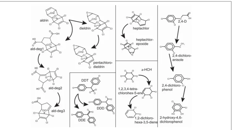
Fig. 1: Degradation Pathways for the five substances in this study
by CATABOL. In the degradation pathways that we have selected for this assessment, we have retained only substances for which this probability was greater than 0. This was the case for between six (aldrin) and two (heptachlor) substances. The selected degradation pathways in soil are shown in Fig. 1. Degradation pathways predicted by CATABOL are subject to considerable uncertainty. For aldrin, e.g., Paasivirta et al. (1988) have identified transformation products that are not indicated by CATABOL. We have, in this case, changed the pathways predicted by CATABOL to include pentachloro-dieldrin, as suggested by Paasivirta et al. (1988).
Biodegradation is representative for the degradation pro-cesses in soil, and to a certain amount also in water and vegetation. In the atmosphere, OH radical reactions are the most important degradation pathway, and they do not nec-essarily form the same products as biodegradation. Unfor-tunately, there is to our knowledge no QSAR software avail-able that would predict the substances formed after OH radical reactions. Therefore, if no literature information was available, we have assumed that OH radical reactions al-ways lead to total mineralization of the substance. This leads to an underestimation of the total hazard caused by those chemicals. This meant that α-HCH and 2,4-D were directly mineralized in atmosphere, and that the degradation prod-ucts of dieldrin were mineralized in atmosphere, too. Ald-rin, DDT, and heptachlor were degraded into dieldAld-rin, DDE and heptachlor-epoxide with a fraction of formation of 0.9 (Crosby & Moilanen 1977, Zepp et al. 1977, Buser & Muller 1993, Bandala et al. 2002).
In addition to the degradation pathways, degradation half-lives for all the substances had to be found for the different media. Sometimes such values are measured and reported
(Mackay et al. 1997), but this is not usually the case for degradation products. Therefore, QSAR software was used to predict degradation half-lives if no reported values were available. AOPWin and BIOWin from the EPIWin software (US-EPA 2000) were used to calculate OH reaction rates and biodegradation half-lives. The degradation classes given by BIOWin were transformed into half-lives with the esti-mation procedure suggested by Arnot et al. (2005). Finally, partitioning information for all the substances had to be found. KOW and KAW values have been measured for a large number of substances, and such data has been as-sembled for pesticides by various authors (Beyer et al. 2002, Xiao et al. 2004, Shen & Wania 2005). Here, we have taken an improved compilation of partitioning data and their tem-perature dependency by Schenker et al. (2005). Again, par-titioning data is usually unavailable for degradation prod-ucts that were not known to be persistent. We have relied on QSAR software from the EPIWin package to extract raw values of KOW and KAW. Those values were adjusted with the least-squares adjustment procedure (Schenker et al. 2005). Temperature dependencies were estimated with a method suggested by MacLeod et al. (2007).
Fig. 1 shows the degradation pathways of the selected sub-stances and Table 1 gives the degradation half-lives and the partitioning properties for the selected substances as they were used for the calculations in this paper. As mentioned above, DDT is simultaneously degraded into DDE and DDD in soil and water. In atmosphere, DDT is degraded into DDE only. Aldrin can be degraded in two different ways: either into dieldrin and then pentachlorodieldrin, or it can be de-graded in three steps to more polar substances (ald-deg1 to
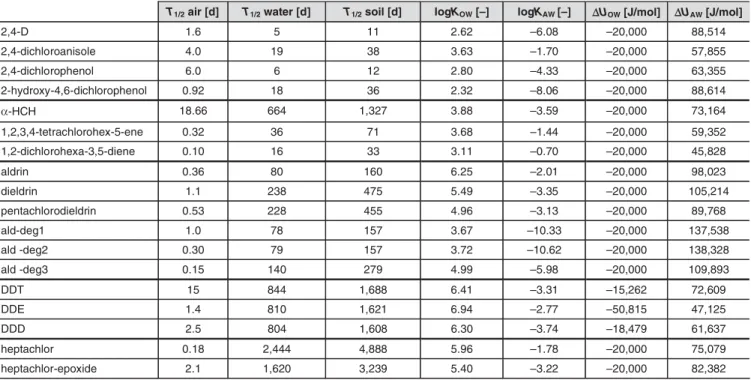
T1/2 air [d] T1/2 water [d] T1/2 soil [d] logKOW [–] logKAW [–] ΔUOW [J/mol] ΔUAW [J/mol] 2,4-D 1.6 5 11 2.62 –6.08 –20,000 88,514 2,4-dichloroanisole 4.0 19 38 3.63 –1.70 –20,000 57,855 2,4-dichlorophenol 6.0 6 12 2.80 –4.33 –20,000 63,355 2-hydroxy-4,6-dichlorophenol 0.92 18 36 2.32 –8.06 –20,000 88,614 α-HCH 18.66 664 1,327 3.88 –3.59 –20,000 73,164 1,2,3,4-tetrachlorohex-5-ene 0.32 36 71 3.68 –1.44 –20,000 59,352 1,2-dichlorohexa-3,5-diene 0.10 16 33 3.11 –0.70 –20,000 45,828 aldrin 0.36 80 160 6.25 –2.01 –20,000 98,023 dieldrin 1.1 238 475 5.49 –3.35 –20,000 105,214 pentachlorodieldrin 0.53 228 455 4.96 –3.13 –20,000 89,768 ald-deg1 1.0 78 157 3.67 –10.33 –20,000 137,538 ald -deg2 0.30 79 157 3.72 –10.62 –20,000 138,328 ald -deg3 0.15 140 279 4.99 –5.98 –20,000 109,893 DDT 15 844 1,688 6.41 –3.31 –15,262 72,609 DDE 1.4 810 1,621 6.94 –2.77 –50,815 47,125 DDD 2.5 804 1,608 6.30 –3.74 –18,479 61,637 heptachlor 0.18 2,444 4,888 5.96 –1.78 –20,000 75,079 heptachlor-epoxide 2.1 1,620 3,239 5.40 –3.22 –20,000 82,382
Table 1: Degradation half-lives (T1/2), partition coefficients (logKOW, logKAW) and their temperature dependencies (ΔUOW,ΔUAW) for the substances used
in this study
Fig. 2: The geometry of the CliMoChem model
ald-deg3). Heptachlor is degraded into heptachlor epoxide, and α-HCH is de-chlorinated in two steps. Finally, 2,4-D degrades into 2,4-dichloroanisole, and then in two steps into 2-hydroxy-4,6-dichlorophenol.
1.2 The CliMoChem model
CliMoChem (Scheringer et al. 2000, Scheringer et al. 2004, Wegmann 2004, Wegmann et al. 2006) is a zonally aver-aged multi-media box model. The model assembles a vari-able number of zones in the North-South direction (Fig. 2). Each of the zones represents one latitudinal band around the globe and is composed of an ocean-water, atmosphere, bare-soil, vegetation-soil and vegetation compartment. The model assumes a homogeneous distribution of the chemi-cals in the East-West direction. The model calculates envi-ronmental processes such as diffusive exchange between phases (partitioning), advective exchange between phases (wet deposition, runoff), transport between zones (wind, ocean-currents), and degradation. For each box (a compart-ment in a zone), mass-balance equations can be written to describe the exchange, transport, emission, and degradation processes (for details, see (Scheringer et al. 2000)). The mass-balance equations for a given substance in all the boxes can be summarized in a single differential equation with a
square-matrix S, see eq. 1. S stores all the above-mentioned pro-cesses for all the boxes in the model and has the size (nzones *
ncompartments) * (nzones * ncompartments); c(t) and dc(t)/dt are vec-tors with (nzones * ncompartments) elements.
(Eq. 1) Fenner et al. (2000) have shown how a series of chemicals can simultaneously be calculated with the above equations for a unit world model. This procedure can be applied as such for the case of a zonally averaged model and is recon-structed briefly here. For each substance X, the mass bal-ance equations have to be established as mentioned above, leading to a series of SX matrixes. To link the substances
with each other, the SX matrixes have to be written as blocks
on the diagonal of a new SBIG matrix. The non-diagonal blocks of the SBIG matrix have to be filled with source ma-trixes. Those source matrixes contain on their diagonals the
ki degradation coefficients multiplied by the respective frac-tions of formation ffi->j (for the degradation of the parent
compound i into the degradation product j, as described in the previous section).
1.3 Expanding exposure-based hazard indicators to take degradation products into account
Exposure-based hazard indicators have been developed to classify chemical substances according to their persistence, long-range transport potential and probability to accumu-late in the arctic.
At steady-state (with continuous emissions of a parent com-pound of m, in kg/day), the primary persistence (PP), as de-fined in Scheringer (1996), is the total mass of the parent compound in the system divided by the emission rate m.
( )
( )
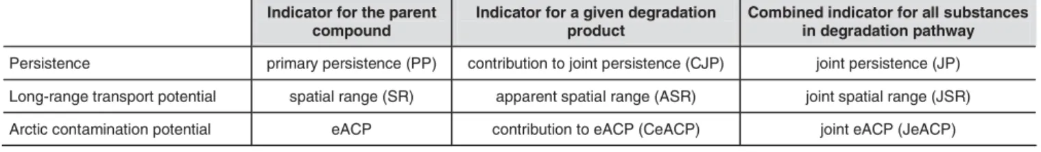
t dt t d c S c ⋅ =Indicator for the parent compound
Indicator for a given degradation product
Combined indicator for all substances in degradation pathway
Persistence primary persistence (PP) contribution to joint persistence (CJP) joint persistence (JP) Long-range transport potential spatial range (SR) apparent spatial range (ASR) joint spatial range (JSR) Arctic contamination potential eACP contribution to eACP (CeACP) joint eACP (JeACP)
Table 2: Overview of the indicators for parent compounds, degradation products, and combined indicators for all the substances in the degradation pathway
Fig. 3: Evolution of the concentration of DDT and its degradation products
after a pulse emission. The plot shows the evolution in the emission zone at the equator in soil as a function of time (in years)
The primary persistence represents the overall residence time of the chemical in the system. In analogy, Fenner et al. (2000) have defined the joint persistence (JP) as the overall resi-dence time of the parent compound and all its degradation products in the system. At steady-state, it can be calculated as the sum of the mass of the parent compound and all the degradation products divided by the emission rate m (of the parent compound). The 'contribution to joint persistence' (CJP) of the degradation products, finally, is the steady-state mass of a given degradation product, divided by m. It can easily be seen that the sum of the contributions to joint per-sistence of all the degradation products, plus the primary persistence of the parent compound is equal to the joint per-sistence (PP + ΣiCJPi = JP). These concepts are equally valid
for pulse emissions that we have worked with in this project. The spatial range (Scheringer 1997) serves to classify chemi-cals according to their long-range transport potential. It is defined as the 95% interquantile range of the geographical distribution of the time-integrated mass on a north-south transect of the earth, after an emission at the equator. A high spatial range signifies that a substance is highly mobile and will be transported far away from the usage areas. It has been shown that this concept can be expanded for deg-radation products, too (Quartier & Müller-Herold 2000). In analogy to the joint persistence, we define here the joint spatial range as the 95% interquantile range of the sum of the time-integrated mass of the parent compound and all the degradation products. In analogy to the 'contribution to joint persistence', we define an indicator for the individual degradation products, too: the 'apparent spatial range' is defined as the 95% interquantile range of a given degrada-tion product after the emission of the parent compound. This 'apparent spatial range' of a degradation product is not equal to the spatial range of the same substance if it were directly emitted at the equator. It can be shown that the joint spatial range must lie within the minimum and the maximum of the spatial range of the parent compound and the apparent spatial ranges of all the degradation products. The Arctic Contamination Potential (ACP) has been intro-duced to identify chemicals that are likely to accumulate in the Arctic (Wania 2003). In the current project, we work with the exposure-ACP (eACP), as opposed to the mass-ACP (mmass-ACP); see Wania (2004). The emass-ACP has been de-fined as the ratio of the mass of a chemical that is present in the arctic surface media (excluding atmosphere), divided by the total emissions of the substance, after 1 year (eACP-1), and after 10 years (eACP-10). The emissions of the sub-stances occur proportionally to the latitudinal population distribution over the globe. In analogy to the joint persis-tence and the joint spatial range, we define the joint eACP
as the ratio of the total mass of the parent compound and the mass of all the degradation products, divided by the to-tal emissions of the parent compound. Like the contribu-tion to the joint persistence, the contribucontribu-tion to the joint eACP can be calculated for the degradation products. The joint eACP is again the sum of the eACP of the parent com-pound and the contributions to joint eACP of all the degra-dation products.
All described indicators are sensitive to the medium to which the substance is emitted. In our case, all emissions were into atmosphere. An overview of the nomenclature of the different indicators for parent compounds, individual deg-radation products, and entire substance families is given in
Table 2.
2 Results
2.1 Impact of degradation products on the temporal evolution of concentrations
The temporal evolution of all the substances follows a simi-lar pattern. As an example, Fig. 3 displays the evolution of DDT and its degradation products DDE and DDD. It can be seen how the concentration of DDT decreases immedi-ately after the pulse emission, and continues to decrease ex-ponentially. The two degradation products DDE and DDD are present at low concentrations at the beginning and ac-cumulate in the first years, as a result of the degradation of DDT. After about 3–4 years, their concentration has reached a peak, and they start to decrease, too, although at a slower rate than DDT. Eventually (after about 10 years), DDE and DDD are present at higher concentrations than DDT.
Fig. 5: Spatial Range of the studied substances. The spatial range of the parent compound is given in gray, the apparent spatial range of the degradation
products in white, and the joint spatial range in black. The apparent spatial ranges of the two α-HCH degradation products are 96 and 98% and are not completely displayed in the figure
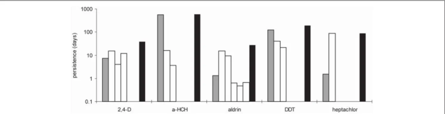
Fig. 4: Persistence (in a log-scale) of the studied substances: parent compounds have gray bars, their degradation products white bars, and the joint
persistence of the whole substance family is given in black bars For the other substance families, a similar behavior can be observed: for heptachlor, for instance, the degradation prod-uct is present at higher concentrations than the parent com-pound already after only a few months, because the half-life of heptachlor-epoxide is so much longer than the one of the parent compound. Later on, the concentration of the degra-dation product is several magnitudes higher than the con-centration of the parent compound. In the environment, this would mean that the degradation product would be present in much higher concentrations than the parent compound (a finding that is confirmed, for instance, for measurements in arctic atmosphere (Hung et al. 2005) or in temperate ag-ricultural soils (Harner et al. 1999)).
2.2 Persistence
Fig. 4 gives the persistence for the five parent compounds
and their degradation products, and the joint persistence. It is clearly visible that the persistence of aldrin and heptachlor is significantly increased if their degradation products are included. The impact is still significant for the herbicide 2,4-D, but for DDT and especially for α-HCH, the increase of the persistence is of less than a factor two. This is consistent for the case of α-HCH (a substance that is not known to have persistent degradation products), but surprising for DDT, as DDE is often cited as an example for an important degra-dation product. One reason why the hazard of DDE might be underestimated in our study is that the half-life in atmo-sphere for DDE is based only on one QSAR value from AOPWin (1.4 days). For DDT, in addition to the AOPWin
value, several estimated and measured atmospheric half-lives were available (Moltmann et al. 1999, Liu et al. 2005, Müller 2005). These alternative values suggest a much slower deg-radation (20.9 days on average) than indicated by the AOPWin value for DDT (that is similar to the QSAR result of DDE: 3.1 days), and therefore the atmospheric half-life of DDT in our study is much higher than the one of DDE, see Tab. 1. If alternative values for the half-life of DDE were available, they would probably be significantly higher than the AOPWin value, too. This would significantly increase the contribution to joint persistence for DDE.
2.3 Spatial Range
Fig. 5 shows that the apparent spatial range of many
degra-dation products exceeds the spatial range of the parent com-pound. This effect is very significant for the α-HCH, hep-tachlor, 2,4-D, and DDT substance families, but less pro-nounced for the aldrin substance family. The joint spatial range of α-HCH (and DDT) is almost uninfluenced by the degradation products, although those have very high appar-ent spatial ranges (especially for the case of α-HCH). This will be analyzed in detail in the discussion part.
2.4 Arctic contamination potential
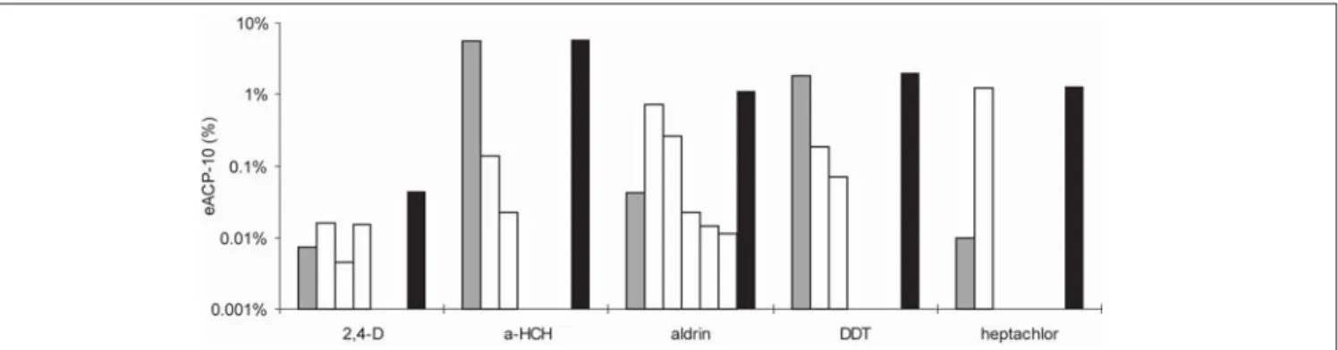
As could already be seen for the persistence, the degrada-tion products of aldrin and heptachlor considerably increase the eACP-10 of their parent compounds (Fig. 6). For α-HCH and DDT, the effects are much less pronounced.
Fig. 6: Arctic contamination potential after 10 years (eACP-10), for the parent compound (gray), the degradation products (white), and the joint ACP for
the whole substance family (black). The scale is a log-scale and gives the eACP-10 in percents
3 Discussion
The contribution of degradation products to persistence has previously been assessed with unit world models (Fenner et al. 2000). Our study confirms the findings from the previ-ous work: for some substances (such as heptachlor and ald-rin), the impact of the degradation products is very impor-tant, as the joint persistence is much higher than the primary persistence of the parent compound (a factor of 20 for ald-rin and 58 for heptachlor). For other substances, like DDT and especially α-HCH, the impact is much lower, for α-HCH the increase is only by 4%. This is because the two degrada-tion products of α-HCH, 1,2,3,4-tetrachlorohex-5-ene and 1,2-dichlorohexa-3,5-diene, are chemicals that degrade quite readily in the environment. These results show that the per-sistence of the parent compound alone is not a good indica-tor for the joint persistence of the whole substance family. Many degradation products have a higher apparent spatial range than the parent compound. This can be explained by the fact that the parent compound is emitted as a pulse emis-sion at the equator, whereas the degradation products occur continuously on the whole globe, as a result of the transport of the parent compound. The joint spatial range for hep-tachlor and 2,4-D is much higher than the spatial range of their parent compounds (a factor of 3.5 and 2.4). This shows again that the spatial range of the parent compound is not a good indicator for the long-range transport potential of the whole substance family.
Interestingly, for aldrin, DDT, and α-HCH, the joint spatial range is almost equal to the one of the parent compound, although the apparent spatial ranges of the degradation prod-ucts are much higher. This is due to the fact that the contri-bution to joint persistence of those intermediate degrada-tion products is very low: they are present in the system in relatively small quantities. The joint spatial range, as it is defined, is mainly determined by the substance that is present at the highest concentrations, which is the parent compound for the case of α-HCH. In the case of heptachlor, the degra-dation product is present at much higher concentrations, and therefore, the joint spatial range is determined by the degradation product. It can therefore be said, if persistent degradation products that are subject to long-range trans-port exist, that the joint spatial range will be significantly higher than the spatial range of the parent compound.
The arctic contamination potential shows a behavior simi-lar to the one for joint persistence: for aldrin and heptachlor, an important increase of the eACP-10 can be observed, while the difference is only minor for DDT and α-HCH. This stresses again the fact that the eACP-10 of the parent com-pound can, in some cases even severely, underestimate the overall hazard of a substance family: including heptachlor-epoxide in the 10 of heptachlor increases the eACP-10 by a factor of more than eACP-100.
In the current study, we have heavily relied on estimation methods to determine substance parameters and degrada-tion pathways. Our conclusions can therefore only highlight the general importance of degradation products, especially with respect to the three indicators investigated. To confirm the accuracy of the predictions of our model, and to be able to draw conclusions on a specific substance, more thorough studies are required that have to include a comprehensive investigation of the degradation pathways and the substance properties as well as detailed comparisons of model results and measurements in various environmental media and re-gions of the world. For DDT, we are presently working on such a study (Schenker et al. 2007), taking into account his-torical emissions, measured data on chemical properties and degradation kinetics, and conducting a detailed comparison of model results and concentrations measured in the field. This study on DDT demonstrates that the CliMoChem model yields results that are in good agreement with field data.
4 Conclusions
The importance of degradation products for the hazard as-sessment of organic chemicals has clearly been shown. Tak-ing into account only the parent compounds can lead to a severe underestimation of the persistence, the spatial range and also the arctic contamination potential. Furthermore, for regulatory purposes, chemicals are often ranked accord-ing to their score for persistence, spatial range or arctic con-tamination potential. The goal of this is to identify the most harmful substances. If such a ranking is uniquely based on the score of the parent compound, it is well possible that substances with low scores for their parent compounds, but high scores for the degradation products would not be iden-tified, whereas substances with a high score for the parent compound, but very low score for the degradation products would be flagged as problematic.
5 Recommendations and Perspectives
It is suggested that degradation products be included in haz-ard assessments to gain a more accurate insight into the en-vironmental hazard of chemicals. The findings of this project could also be combined with information on the toxicity of degradation products. This would provide further insight into the importance of degradation products for environ-mental risk assessments.
Acknowledgement. We gratefully acknowledge the help of Mark
Bonnell, Lukas Gasser and Kathrin Fenner in the compilation of the degradation pathways, and thank Fabio Wegmann for interesting com-ments on the project.
References
AMAP (1998): AMAP Assessment Report – Arctic Pollution Issues. Arctic Monitoring and Assessment Program (AMAP), Oslo
Arnot J, Gouin T, Mackay D (2005): Practical Methods for Estimating En-vironmental Biodegradation Rates, Canadian EnEn-vironmental Modelling Network, Peterborough
Bandala ER, Gelover S, Leal MT, Arancibia-Bulnes C, Jimenez A, Estrada CA (2002): Solar photocatalytic degradation of Aldrin. Catal Today 76, 189 Beyer A, Wania F, Gouin T, Mackay D, Matthies M (2002): Selecting
inter-nally consistent physicochemical properties of organic compounds. Environ Toxicol Chem 21, 941–953
Boxall ABA, Sinclair CJ, Fenner K, Kolpin D, Maud SJ (2004): When syn-thetic chemicals degrade in the environment. Environ Sci Technol 38, 368A–375A
Buser HR, Muller MD (1993): Enantioselective Determination of Chlor-dane Components, Metabolites, and Photoconversion Products in Envi-ronmental-Samples Using Chiral High-Resolution Gas-Chromatography and Mass-Spectrometry. Environ Sci Technol 27, 1211
Cahill TM, Cousins I, Mackay D (2003): General fugacity-based model to predict the environmental fate of multiple chemical species. Environ Toxi-col Chem 22, 483–493
Crosby DG, Moilanen KW (1977): Vapor-Phase Photodecomposition of DDT. Chemosphere 6, 167–172
Dachs J, Lohmann R, Ockenden WA, Mejanelle L, Eisenreich SJ, Jones KC (2002): Oceanic biogeochemical controls on global dynamics of persis-tent organic pollutants. Environ Sci Technol 36, 4229–4237
Ellis LBM, Roe D, Wackett LP (2006): The University of Minnesota Biocatalysis/Biodegradation Database: the first decade. Nucleic Acids Res 34, D517
Fenner K, Scheringer M, Hungerbuhler K (2000): Persistence of parent com-pounds and transformation products in a level IV multimedia model. Environ Sci Technol 34, 3809–3817
Fenner K (2001): Transformation Products in Environmental Risk Assess-ment: Joint and Secondary Persistence as New Indicators for the Overall Hazard of Chemical Pollutants. PhD Thesis, Swiss Federal Institute of Technology Zurich, Zurich, Switzerland
Harner T, Wideman JL, Jantunen LMM, Bidleman TF, Parkhurst MJ (1999): Residues of organochlorine pesticides in Alabama soils. Environ Pollut 106, 323
Hung H, Blanchard P, Halsall CJ, Bidleman TF, Stern GA, Fellin P, Muir DCG, Barrie LA, Jantunen LM, Helm PA, Ma J, Konoplev A (2005): Temporal and spatial variabilities of atmospheric polychlorinated biphe-nyls (PCBs), organochlorine (OC) pesticides and polycyclic aromatic hy-drocarbons (PAHs) in the Canadian Arctic: Results from a decade of monitoring. Sci Total Environ 342, 119
Jaworska J, Dimitrov S, Nikolova N, Mekenyan O (2002): Probabilistic assessment of biodegradability based on metabolic pathways: Catabol system. SAR QSAR Environ Res 13, 307
Koziol AS, Pudykiewicz JA (2001): Global-scale environmental transport of persistent organic pollutants. Chemosphere 45, 1181–1200
Leip A, Lammel G (2004): Indicators for persistence and long-range trans-port potential as derived from multicompartment chemistry-transtrans-port modelling. Environ Pollut 128, 205
Liu Q, Krüger HU, Zetzsch C (2005): Degradation study of the aerosol-borne insecticides Dicofol and DDT in an aerosol smog chamber facility
by OH radicals in relation to the POPs convention. Proceedings to Euro-pean Geosciences Union in Vienna, Austria
Mackay D, Paterson S (1991): Evaluating the Multimedia Fate of Organic-Chemicals – A Level-III Fugacity Model. Environ Sci Technol 25, 427–436 Mackay D, Shiu WY, Ma KC (1997): Illustrated Handbook of Physical-Chemical Properties and Environmental Fate for Organic Physical-Chemicals, Vol 5. Lewis Publishers, Boca Raton
MacLeod M, Scheringer M, Hungerbühler K (2007): Estimating enthalpy of vaporization from vapor pressure using Trouton's rule. Environ Sci Technol (in press)
Moltmann JF, Küppers K, Knacker T, Klöpffer W, Schmidt E, Renner I (1999): Verteilung persistenter Chemikalien in marinen Ökosystem, ECT Oeko-toxikologie GmbH, Floersheim am Main
Müller M (2005): Gutachten zur Validierung von QSAR-Modellen zur Ab-schätzung des atmosphärischen Abbaus mit einem Datensatz von ca. 760 Stoffen, Frauenhofer-Institut für Molekularbiologie und Angewandte Oekologie, Schmallenberg, Germany
Paasivirta J, Palm H, Paukku R, Akhabuhaya J, Lodenius M (1988): Chlo-rinated Insecticide Residues in Tanzanian Environment – Tanzadrin. Chemosphere 17, 2055–2062
Quartier R, Müller-Herold U (2000): On secondary spatial ranges of trans-formation products in the environment. Ecol Model 135, 187–198 Schenker U, MacLeod M, Scheringer M, Hungerbühler K (2005):
Improv-ing Accuracy and Quality of Data for Environmental Fate Models: A Least-Squares Adjustment Procedure for Harmonizing Physicochemical Properties of Organic Compounds. Environ Sci Technol 39, 8434–8441 Schenker U, Scheringer M, Hungerbühler K (2007): Modeling DDT in a global fate model: Reproducing current levels, looking out into the fu-ture. Environ Sci Technol (submitted)
Scheringer M (1996): Persistence and spatial range as endpoints of an expo-sure-based assessment of organic chemicals. Environ Sci Technol 30, 1652– 1659
Scheringer M (1997): Characterization of the environmental distribution behavior of organic chemicals by means of persistence and spatial range. Environ Sci Technol 31, 2891–2897
Scheringer M, Wegmann F, Fenner K, Hungerbühler K (2000): Investigation of the cold condensation of persistent organic pollutants with a global multimedia fate model. Environ Sci Technol 34, 1842–1850
Scheringer M, Salzmann M, Stroebe M, Wegmann F, Fenner K, Hungerbühler K (2004): Long-range transport and global fractionation of POPs: In-sights from multimedia modeling studies. Environ Pollut 128, 177–188 Schmidt M (1996): University of Minnesota biocatalysis biodegradation
database. Asm News 62, 102
Shen L, Wania F (2005): Compilation, Evaluation, and Selection of Physi-cal-Chemical Property Data for Organochlorine Pesticides. J Chem Eng Data 50, 742–768
UNEP (2001): Homepage of the Stockholm Convention on Persistent Or-ganic Pollutants. Secretariat for the Stockholm Convention on Persistent Organic Pollutants. <http://www.pops.int/>
US-EPA (2000): EPIWin Suite. Syracuse Research Corporation. <http:// www.epa.gov/oppt/p2framework/docs/epiwin.htm>
Wania F, Mackay D (1995): A Global Distribution Model for Persistent Organic-Chemicals. Sci Total Environ 161, 211–232
Wania F (2003): Assessing the potential of persistent organic chemicals for long-range transport and accumulation in polar regions. Environ Sci Technol 37, 1344–1351
Wania F (2004): Schadstoffe ohne Grenzen – Ferntransport persistenter organischer Umweltchemikalien in die Kälteregionen der Erde. GAIA 13, 176–185
Wegmann F (2004): The Global Dynamic Multicompartment Model CliMoChem for Persistent Organic Pollutants: Investigations of the Veg-etation Influence, the Cold Condensation and the Global Fractionation. PhD Thesis, Swiss Federal Institute of Technology, Zurich, Switzerland Wegmann F, Scheringer M, Hungerbühler K (2006): First investigations of
mountainous cold condensation effects with the CliMoChem model. Ecotoxicology and Environmental Safety 63, 42–51
Xiao H, Li NQ, Wania F (2004): Compilation, evaluation, and selection of physical-chemical property data for alpha-, beta-, and gamma-hexachlo-rocyclohexane. J Chem Eng Data 49, 173–185
Zepp RG, Wolfe NL, Azarraga LV, Cox RH, Pape CW (1977): Photochemi-cal Transformation of DDT and Methoxychlor Degradation Products, DDE and DMDE, by Sunlight. Arch Environ Contam Toxicol 6, 305–314
Received: December 12th, 2006 Accepted: March 14th, 2007