by
JAMIE C. CHAPMAN
B.A., University of California, Santa Barbara (1958)
M. S., Case Institute of Technology (1961)
SUBMITTED IN PARTIAL FULFILLMENT OF THE REQUIREMENTS FOR THE
DEGREE OF DOCTOR OF PHILOSOPHY
at the
MASSACHUSETTS INSTITUTE OF TECHNOLOGY June, 1966
Signature of Author ...
Deparyment of Geology and Geophysics May 13, 1966
Certified by . . . . Thesis Supervisor
Accepted by . . . . Chairman, Departmental Committee
ABSTRACT
Considered was the scattering of a particle of charge q and mass m in a uniform magnetic field by the Coulomb potential of a charge Q fixed at the origin. The scattering was described quantum-mechanically by a formalism in which the presence of the magnetic field was incorporated as the dominant and controlling factor. Also incorporated was the facility for varying the initial position of the gyrocenter with respect to the line on which the scattering charge is located, and for keeping track of the energies perpendicular and parallel to the magnetic field.
The charge q was represented in a Born approximation cross section by combinations of the energy eigenfunction set obtained as solutions to the Schroedinger equation H = E in a
o NMk o NMk
_ 2 cylindrical coordinate system. The Hamiltonian H = (p - qA) /2m
0
is that describing the motion of a single particle in the magnetic field generated from the potential A. The parameters (NMk) are interpre-ted in terms of energies perpendicular and parallel to the magnetic field and in terms of the radius and radial position of the corresponding classical orbits.
An exact result was obtained for the matrix element of the Coulomb potential energy between these eigenfunctions. The diagonal matrix element is characterized by a logarithmic singularity. The maximum value of the off-diagonal element used in the scattering
cal--10
culations was about 10 eV - m. A simple, limiting form was ob-tained and utilized in a differential cross section.
ACKNOWLEDGEMENT
The existence of this thesis is due in large and substantial part to the prodding, help and encouragement of four persons: Francis Bitter and Giorgio Fiocco of the Department of Geology and Geophysics; Hernan Praddaude of the National Magnet Labora-tory at MIT; and John Champeny of EG&G, Inc.
Work on this thesis was supported in part by the Research Laboratory of Electronics and by the National Magnet Laboratory at MIT. Figures C1 and C2 were made through the facilities of the MIT Computation Center.
TABLE OF CONTENTS TITLE PAGE ... ... ... i ABSTRACT .... ... .... ... ... .. ... ... ii ACKNOWLEDGEMENTS ... ... iii TABLE OF CONTENTS ... iv LIST OF FIGURES ... ... ix LIST OF TABLES... ... ... x
PART I: SUMMARY PAPER I. INTRODUCTION... ... 2
C ontent .... .. ... . .... .. ... .... 2
Context ... 5
II. THE CYLINDRICAL LANDAU EIGENFUNCTIONS. ... 8
Properties ... ... .. ... 8
Interpretation of the Eigenparameters (NMk). ... 9
III. THE COULOMB MATRIX ELEMENT ... .10
IV. BORN APPROXIMATION CROSS SECTIONS. ... 13
AND MAGNETIC FIELDS ... 17
Al Introduction ... ... 17
A2 The Lagrangian Formalism ... 18
The Non-relativistic Lagrangian ... 18
The Relation of Canonical and Linear Momenta. .. .19
Application to Cylindrical Coordinates. ... 20
Equations of Motion ... 23
A3 The System Hamiltonian ... 24
Construction of the Hamiltonian ... 24
Equations of Motion ... 25
A4 Numerical Estimates of Hamiltonian Energies and Other Quantities of Interest ... 26
A5 The Effect of Coordinate System Rotation ... 29
Rationale ... 29
Lagrangian-Hamiltonian Formalism in Rotating Coordinates ... .... ... 30
The Lagrangian Equations of Motion ... 34 B SOME FEATURES OF THE CLASSICAL MOTION OF
A CHARGED PARTICLE IN A MAGNETIC FIELD ... B 1 C ontent . . . . B2 Coordinates of the Perpendicular Motion ...
B3 Constants of the Motion ...
B4 Three Time-Averaged Dynamical Variables... Squared Distance, Origin to Particle ... Radial and Azimuthal Components of the
Perpendicular Energy . ... ... .36 36 .36 .37 .40 .40 41
C A QUANTUM REPRESENTATION OF A CHARGED PARTICLE IN A MAGNETIC FIELD: THE CYLINDRICAL LANDAU
EIGENFUNCTIONS ... ... ... 45
C1 Introduction ... ... .. ... 45
C2 Derivation and Properties ... ... 45
C3 Interpretation of the Quantum Numbers and Parameters ... ... ... 55
The Wavenumber k of the z Eigenfunctions ... .55
Density in Energy of the z Eigenstates. ... 56
The Quantum Number M of the Azimuthal or <. Eigenfunctions. ... 57
The Signs of <} and the Radial Quantum Number N .... ... . . ; ... .. 57
Degeneracy of the Perpendicular Energy Levels. .62 Surfaces of Constant Energy. ... 63
C4 Construction of a Uniform Beam . ... .... 67
De finition and Representation ... 68
Position Upon the Surfaces of Constant Energy. . . 69
Normalization and z Flux ... ... . 69
C5 Sum m ary. ... ... 70
D MATRIX ELEMENTS OF RADIAL POSITION AND ENERGY BETWEEN CYLINDRICAL LANDAU EIGENFUNCTIONS... 73
D 1 Content ... .. .. .... . ... . ... 73
D2 The Set of Basis Eigenfunctions ... 74
D3 The Matrix Element < ... 75
Case a = 0. The Normalization Integral. ... .77
Case o = 1. The Matrix Element <q > ... 78
Case a' = -1. The Matrix Element <(W)'> .. .... 78
E EVALUATION OF THE COULOMB MATRIX ELEMENT
BETWEEN CYLINDRICAL LANDAU EIGENSTATES. ... 82
El Content ... 82
The Centered Coulomb Matrix Element. ... 82
The Off-Center Coulomb Matrix Element. ... .84
E2 Execution of the Centered Coulomb Matrix Element . 86 Method I ... 88
Two Alternate Methods ... 92
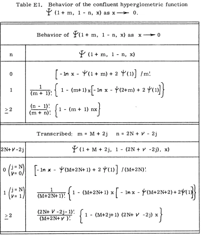
E3 Properties of the Confluent Hypergeometric Psi Function ... 95
General Relations ... 95
The Particular Form of Interest. .. ... 97
Leading Terms for Small Values of the Argument ... ... 98
Behavior for Large Values of the Argument. .. . 101
General Behavior. ... .101
Computation ... ... . 102
E4 Variation of the Argument Y ... 105
E5 Behavior and Properties of the Centered Coulomb Matrix Element ... 110
The Diagonal Matrix Element ... 111
The Off-Diagonal Matrix Elements ... 112
E6 The Centered Coulomb Matrix Element in the Limit of Small Angle Scattering ... 116
F PROBABILITY DENSITY FLUX ASSOCIATED WITH THE CYLINDRICAL LANDAU EIGENFUNCTIONS ... 122
F1 Content ... ... ... 122
F2 Origin of the Flux Concept, and General Expressions ... .... ... .. .... .122
F3 Flux Associated with Cylindrical Landau Eigenfunctions ... ... ... 123
G DERIVATION OF THE DIFFERENTIAL CROSS SECTION
FOR SCATTERING IN A MAGNETIC FIELD. ... 128 G1 Introduction ... ... . 128 G2 General Formalism ... 128 G3 Application to Cylindrical Landau Eigenfunctions ... 133 G4 Separation of the Two-Particle Hamiltonian... .136 REFERENCES . ... 140 BIOGRAPHICAL NOTE ... 143
LIST OF FIGURES B1 Coordinates used in classical
averages-over-orbits... 38 B2 Results of classical averages
over a cyclotron orbit ... 42 C1 Radial probability density for
several cylindrical Landau
eigenfunctions ... ... 53 C2 Radial probability density for
several cylindrical Landau
eigenfunctions ... ... 54 C3 Surfaces of constant energy for
group I and group II cylindrical
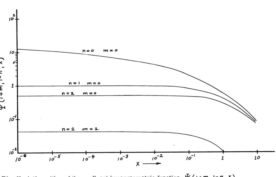
Landau eigenfunctions for q = -e. ... 64 El Variation with x of the confluent
hypergeometric function
F'
(l+m, -n, x)for several values of m and n ... 103 E2 Variation of the argument Y
of the centered Coulomb matrix element, with conservation of
energy incorporated. Approximately
to scale. . . . ... .. 108 E3 Sketch indicating the variation of the
off-diagonal centered Coulomb matrix element, with conservation of energy
Al Numerical estimates of Hamiltonian Energies and other quantities of interest, and comparison for the extreme cases of a bound and an unbound
electron in a uniform magnetic field ... 28 C1 Classification and perpendicular eigenvalues
of the cylindrical Landau eigenfunctions VNMk ... . 60 C2 Eigenstate expectation values of the cylindrical
Landau eigenfunctions ' .NMk . ... 61 El Behavior of the confluent hypergeometric function
( (+m, I-Y,x) as x--O... 100 E2 Properties of the function Y near the origin and at
the end points of the independent variable (N1-N 2 ) / Nz ,
PART I
I. INTRODUCTION
Content
The problem of interest here is the scattering of a charge q in a uniform magnetic field by the Coulomb potential of a charge Q fixed at the origin. The treatment has revealed novel features not present in the zero magnetic field Rutherford problem. The
scattering is described quantum-mechanically by a formalism in which the presence of the magnetic field has been incorporated as the dominant and controlling factor. If there is present any magnetic field, no matter how small, this is the only correct approach. The principal physical reason is the very omnipresence of the magnetic field. Even though the Coulomb potential may be considered long range in character, its influence must eventually become inconsequen-tial as the scattered charge moves farther away along the magnetic field. Also incorporated into the formalism is the facility for varying the initial position of the gyrocenter with respect to the line on which the scattering charge is located, and for keeping track of the energies perpendicular and parallel to the magnetic field. At the heart of the scattering calculations presented herein is the matrix element of the Coulomb potential energy between Schroedinger wave functions repre-senting the scattered particle. An exact result has been obtained for this quantum average. The end result is expressed in terms of a Born approximation cross section. Within limits to be discussed later, the general validity of the results are dependent not upon the
size of the magnetic field, but upon its existence. Indeed, the results simplify considerably for small magnetic fields. The treatment is
spin-less and non-relativistic. Other than these, the chief approximations are connected with the fact that we have ignored the coupling of the relative and center of mass motions, and have ignored the possible
Specifically, and in more detail, the charge q was represented by combinations of the energy eigenfunction set obtained as solutions of the Schroedinger equation
H0 'kmmk -E 34Mk (1)
in the cylindrical coordinate system spanned by the unit vectors
A A A
f x = z. The Hamiltonian Ho is that describing the motion (see Appendix A) of a single particle of charge q and mass m in a magnetic
field:
Ho - (2)
The magnetic field was generated from the vector potential
A
- (3)through the relation
- c url A = (4)
Since the divergence of this potential is identically zero, we may utilize the commutator [, T ] = 0 to combine the two cross terms
of (2). We note specifically that the term quadratic in A (in Be)
is retained. The radial Location of the gyrocenter and the perpendicular and parallel energies are described by the set of eigenparameters
(NMk). We shall see that there are actually two orthogonal sets of such eigenfunctions, one corresponding to cyclotron orbits which enclose the origin and a second describing those which do not.
The Coulomb potential energy, with exponential or Debye shielding incorporated, has the functional form (mks rationalized units are employed):
-4-Q e-4. r
-A-c
L.1X). 0
evr
(5)where r is to be replaced by e' o . This is the potential energy of the charge q (Located at 7) due to Q fixed at the origin. This is the agent or perturbation considered to cause transitions from one
quantum representation of the charge q to another.
Two such representations were employed in the cross section calculations. One was a single eigenfunction 3'NMk ' leading to a differential cross section. The second representation considered, although not as extensively, was a uniform, flooding beam of sufficient radial extent to encompass as much as desired of the Coulomb potential field. This beam, characterized not only by its radial extent but also by single values of the perpendicular and parallel energies, is of use in the consideration of a total cross section.
One of the novel features of this problem is that we are dealing with transitions from a one dimensional continuum in which are embedded discrete states to a second such continuum-discrete system. The
continuum states are associated (through the eigenparameter k) with the free or unbound motion of the charge q along the direction of the magnetic field. The discrete states (belonging to the quantum numbers N and M) are a manifestation of the binding of q by the magnetic field in the plane perpendicular to the field. The transition probability and cross section expressions must reflect this circumstance. These expressions must contain, loosely speaking, one-dimensional density of states functions for both the initial and the final z energies and states.
Derived in appendix G is the Born approximation cross section which takes into account this circumstance and which contains these two density of states functions. It is a differential cross section, in a
way not connected with E.1 and to be made clear later. The expression obtained was
c.7 1( 1-4, Ac)+1cM +2r, +I)
e
= ~ E", H"• (6)where w eB/m. The index a refers to the parameters (N Mlk I)
c 11
characterizing the initial state, and 3 the final state set (N2M2 k 2
Conservation of energy between the initial and final states is implied in this expression, since it has been integrated once on dE 2 over an energy-conserving delta function. Also incorporated has been a result not yet mentioned, namely, conservation of the quantum number M in the basic matrix element (+ qhALj). This result, which has a direct
and interesting classical analog, will greatly facilitate formation of a total cross section from the differential expression (6). We return to the results of this investigation after considering other work,and the relation of the scattering and bound state problems.
Context
Although of fundamental interest, this problem and the closely related bound state problem have been little studied. This is in part due to the formidable mathematical difficulties and in part due to Lack of appreciation of the significance of these problems. By the bound
state problem we mean the properties associated with the solutions and energy spectrum of the Schroedinger equation
wherein the terms quadratic in the product of the magnetic field and radial distance are retained. This is commonly known as the problem of the hydrogen atom in a strong magnetic field. However it is obvious from (3) that this is not a complete description. It is also the problem of the hydrogen atom in a (perhaps moderate) magnetic field and with the electron in a highly excited angular momentum state. This is a
most interesting region because the electron, though bound (its wave-function vanishing at infinity in all directions), may have a total positive energy. As the electron occupies states more and more distant from the proton, it may be more strongly bound by the magnetic field than by the Coulomb potential. The always negative and decreasing
(as 1/e ) Coulomb binding energy may be overcome by the always positive and increasing (as e ) magnetic binding energy. The electron
will always be bound in the direction perpendicular to the magnetic field, whether by the Coulomb potential (negative energy) or by the
magnetic field (positive energy). This is not the case along the direction of the magnetic field since the electron does not see the field in this direction. If the electron is bound in this direction, it must have a negative energy, and if not bound, a positive energy. The bound state problem thus approaches the scattering problem as the binding becomes predominantly magnetic in character.
These and other aspects of the bound state problem have been studied by Bitter [1964, 1965, and private communication] and by Praddaude [1964, private communication]. It is probably fair to say that one of the most significant contributions to emerge from their investigations has been the realization that the case of precisely zero magnetic field is singular. That is, the point B = 0 in the treatment of the hydrogen atom as described above is not a limit point as B -- 0. They are separate problems having in common only the Coulomb binding. This may be understood from consideration of the energy eigenvalue
spectrum, some aspects of which already have been discussed above. In an approximate solution to the bound state problem (valid for
S<< I ), Praddaude obtained an energy spectrum of the form
Eb
-
3(1) + P (8)Bitter has obtained a qualitatively similar form by means of semi-classical arguments. The first term is the usual Coulomb binding energy. The second represents the binding by the magnetic field. The quantum number P is related to the angular momentum, or the energy of azimuthal motion. The feature that we wish to emphasize here is that, as B--0, these magnetic field states become more and
more dense (more and more states per unit energy increment). Then, when B = 0, these infinitely numerous states discontinuously
cease to exist. The existence and behavior of this spectrum is a significant feature of the bound state problem, and has profound
implications for the scattering problem. For example, it is conceivable that an electron, initially unbound in the z direction and incident upon a proton, could be temporarily or permanently delayed in its trip along the field line by occupation of one of the states of this spectrum.
Unfortunately, the scattering formalism employed herein is not powerful enough to detect this possibility.
There have been reported sporadic attacks upon the scattering problem, most within the framework of the Born approximation. Each has involved some approximation in the calculation of the matrix elements. Tennenwald [1959) was apparently the first to point out the difficulty of integrating the classical equations of motion and of separating the relative and center of mass motions. Kahn [1960 considered the scattering of Cartesian Landau eigenfunctions against a delta function potential through use of a Greens function in the scattering integral equation. Goldman
Coulomb profiles. problem,
interactions in the calculation of cyclotron radiation line There was found one classical approach to the scattering that of Barananenkov [1960].
II. THE CYLINDRICAL LANDAU EIGENFUNCTIONS
Properties
The cylindrical Landau eigenfunctions INMk' solutions of the Schroedinger equation, (1), are factorable in each of the coordinates as
As derived in appendix C, the factored eigenfunctions have
' 4L R"M ayL e 1M e the forms (10) (11) 2k e' - (12) 2 -2
where 2 eB/2i (dimensions of m-), and N and M are independent positive integers (including zero) having no formal upper bound. Johnson and Lippmann [1949] have identified the reciprocal of 02 (or more precisely 1/2/32) as the minimum area in the x-y plane to which a gyrocenter may be located. It is the minimum area occupied by a single state. We have the numerical relation
* = [7 10
0
(13)
The Laguerre polynomial, an oscillatory function having N zeroes, has the explicit series representation
S(N*t )! (X )
L (x) s 1 (14)
Other equivalent representations are given in equations (C23).
The factored eigenfunctions are separately normalized to Kronecker and Dirac delta functions such that
<N'M'kINk" I N k > S 5m , (k'-k) (15)
r
mk NJ" M)I.,
J<NM
klNMhk> dkQJ 1. (16)From these equations there follows the interpretation that the quantity
j thti(Fr) d-r
ek
(17)represents the probability (a pure number on a scale of unity) of
locating the charge q in the volume element dT at ' = (e, < , z) and in the quantum state characterized by the numbers N and M and the
continuous wavenumber k in the range dk. The appearance of these eigenfunctions is illustrated in Figures C1 and C2 on pages 53 and 54. These or closely related eigenfunctions have been employed by
Dingle[1952], Tannenwald [1959], Goldman [1963, 1964], and Goldman and Oster 11963]. Their relation to the Cartesian Landau eigenfunctions was considered by Johnson and Lippmann [1949].
Interpretation of the Eigenparameters (NMk)
Interpretation of the parameters (NMk) of the cylindrical Landau eigenfunctions follows from construction of the appropriate quantum operators and eigenvalue equations or from quantum-classical corres-pondence arguments. The former is of course the fundamentally correct
method; results obtained by the correspondence method should be verified by construction of the operator eigenvalue equations. The details and results of these procedures are to be found in section C3 (page 55). Although of vital importance to the understanding of what follows, a lucid exposition requires more space than is available here. Because of their importance, it is suggested that the interested
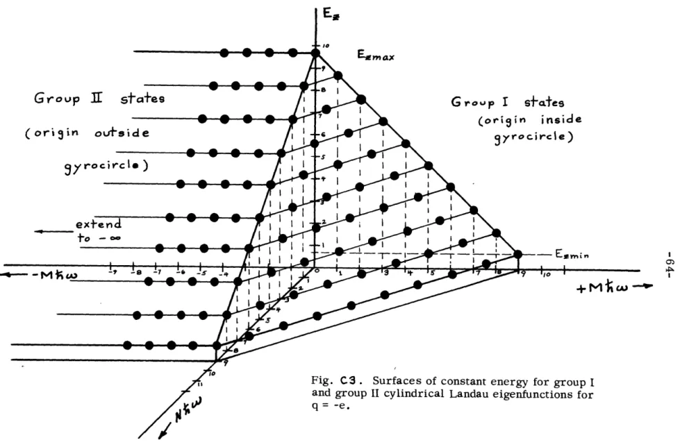
reader pause in this development and consult the ten or so pages of C3. In particular, one should be aware of the role of the + signs of the IM eigenfunctions, understand the distinction between the group I and group II states, and have examined the results summarized in Tables C1 and C2 and in Fig. C3.
III. THE COULOMB MATRIX ELEMENT
The Coulomb matrix element is denoted and defined as
<ZAG>
JA
1 4kMkcr r (18)It was also denoted in (6) by ( , q.~ .+ ). The exact result obtained (section E2) for this integral was
2M. )!+ M)! + M)!
,
2 ") ' " +-) (19)
where
Y
stands for the functions¥II
1.
+,
I± +(N,-z)
(20)
in which conservation of energy has been incorporated and +(1 + m, 1-n, x) denotes a confluent hypergeometric function, the properties of which are discussed in section E3. The parameter N E /i w
is the z energy measured in units of h .. The + signs are associated
c
with forward or back scattering transitions in which the direction of the z momentum is either the same before and after the interaction or is reversed. In what follows, the shielding parameter p is set to zero. The effect of a p > 0 is to depress the values of both forward and back
scattering matrix elements. The properties of the confluent hyper-geometric functions are such that the matrix element for forward scattering transitions is always greater in value than that of the back
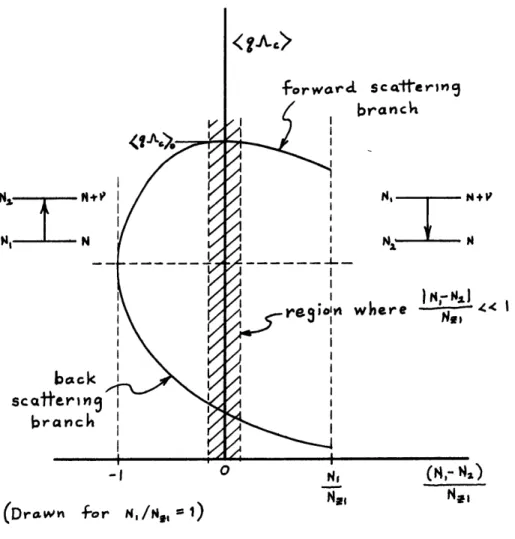
scattering matrix element. The matrix element (19) applies to both group I and group II states even though the signs of IM do not explicitly appear. They are contained implicitly in the interpretation which must be supplied to the quantum integers N and M. The steps leading to the appearance of the Kronecker delta (expressing conservation of the angular momentum canonical to the coordinate , in agreement with the classical equations) indicate that transitions of the type group I group II are explicitly forbidden. Only intragroup transitions are allowed, and only with M conserved. Energy conservation appears in connection with the cross section. The matrix element is symmetric as regards transitions between any pair of states. It was not possible to determine analytically if the matrix element exhibited a preference for equal upward (increase in N) or downward transitions from a given state. These and other properties of this matrix element are explored in sections E4 and E5. The arguements Y are drawn in Fig. E2. The general appearance of the matrix element is sketched in Fig. E3.
The value of an exact result lies not only with the result itself, but also with the fact that it provides a known reference or base from which to make approximations. Because of the analytical complexity of this general result, we shall utilize in the cross section discussions a simplified form in which is embodied the major contribution of the result (19). The simplification proceeds from the fact that, for n
>
1 and any m >, 0, the confluent hypergeometric function j(l+m, 1-n, x)approaches a value independent of x as x -- 0. The form is in essence the constant term of a power series expansion in B V2/E 1 about the origin of the confluent hypergeometric functions of (19). The procedure is described in section E6. The result is
>
(I
(N+M)! (N+P)'(! (N+V+M)!
where V - N1 - N2 and N- min (N1 , N2). Since the minimum values of V, N, and M are respectively 1, 0, and 0, this indicates that the
-10
maximum value of the matrix element (19) is about 10 eV - m. (See equation 5.) The result is valid for V2 /N Z 1, the numerical value of which is
2
for B in w /m and E in eV. This is the principal forward scattering zi
contribution to the matrix element in a region where the back scattering contribution is certainly smaller and may be negligible. As discussed on page 110 in connection with the weaker requirement
V I/N1 <<1, this inequality places no restriction on the size of N 1
relative to Nz1 ( i. e. , the partitioning of the total energy into per-pendicular and parallel modes), but rather is a restriction on the change of the quantum integer N compared to Nz . The milder in-equality is equivalent to the requirement that the relative change in z energy be small, that INz2 - NZ1l /Nzl4<1. We thus have in (21)
a result which describes small angle changes in the momentum vector not only for distant encounters but apparently also for the closest possible encounters (the case M=0, any N and V, is interpreted pictorially or classically as the case where the cyclotron orbit
IV. BORN APPROXIVIATION CROSS SECTION
A cross section is a conversion ratio measuring the efficacy of some agent (here, the Coulomb potential) in transferring the par-ticles or states of an incident beam to some other accessible conditions or states. It may be defined operationally as the number per second w of events (particles, states, or groups of states) arriving at a detector of appropriate configuration, normalized by the product of the incident flux r and the total number of agents N within the scattering
sc volum e:
SNsc r (23)
When the scattering agents operate independently of one another, the number Nsc incorporates and corrects for the additive effect of each independent scatterer upon the detector signal (proportional in some way to w). In theoretical calculations describing single scattering, Nsc
is set to unity, as it is here. By the subscript z we have implied that the predominant direction of the incident flux is along the z axis, which is in this problem the direction of the magnetic field.
Considered here is the cross section for Coulomb scattering of an initial cylindrical Landau eigenstate a = (N 1Mkl ) to a final eigen-state p = (N 2MVIk2). Of interest is the dependence of the cross section
upon the initial energies E_, and Ezl, and upon the initial location of the gyrocenter (in the q-4 plane) with respect to the z axis upon which is located the scattering charge. Also of interest is the most probable change in the perpendicular and parallel energies and the most probable radial gyrocenter displacement. We shall employ the simplified form (21) for the matrix element needed in (6). The
numerical values of (22) indicate that the use of the simplified matrix element does not severely restrict the validity of the final results.
Substitution of the simplified form (21) into (6) yields
M+--N,+I (N+M4)! (N -f)! -FN+V
"=o "V I- + -= N (24)
where the order-of-magnitude coefficient a; is
. WET I - x 1o 1 (25)
SB
The numerical expression bears units of (meters)2 for 1 in w/mn and Ez1 in eV. The explicit B dependence origLnated in expression for the area-averaged flux of the initial eigenstate, While the factor 1/E was contributed by the initial and final one-dimensional density
zl
of z states functions.
The expression (24) is in fact four cross sections since our notation encompasses upward and downward transitions for group I and group II eigenstates. An upward transition is one in which the quantized variables of the perpendicular motion are increased (by V). The principal perpendicular variables of interest are the squared
22 22
gyrocenter distance P C2 and the squared cyclotron radius P e2 (equal to the normalized perpendicular energy E./'uw). The content of the cross sections (24) is more easily understood when they are rewritten in terms of integers directly representing the perpendicular variables:
22
S 2 = 0, 1, 2, . 0 1 (26)
N 2 2 _P =0 1, 2, . (27)
The transformation is accomplished with the aid of the interpretations summarized in Table C1 on page 60. The resulting expressions are listed below. We note that S and N.L refer to initial values, and that
Direction
of Group I
e /e
I Group II e /e Jtransition states or S 4 N-. states or S N. 14.VT s N +l ! (+v ! VN+V!! S (++ S+
N_
o4L+ V)
s,
vZ
(5+p)!S _+5 + INj.- V) 1 SS+ !
N( +I (S-)!
,, " v : (NL- Y)!
For fixed N. and V , both the upward and downward cross sections exhibit qualitatively similar behavior with respect to S. The most significant quantitative difference is that o-t is always greater than -(, except at the value S = N,. The tendency is thus toward outward radial motion with a concomitant increase in the cyclotron radius. As S increases from zero (gyrocircle of squared radius N. centered about the origin, the location of the scattering charge), both cross sections rise from a minimal value (zero for cr, and < o-, for @t ) at the origin to the same maximum value (2N +l)a /V' at the group I-group II boundary point S = N, . This is the single point at which o- = ~ . For all other values of S, Qa t is
invariably greater than- a, . The classical picture associated with the point S = N.L is that of the set of cyclotron orbits of squared radius N,_
whose gyrocenters are situated on the circle of squared radius S = N . That is, S = N., describes the set of orbits which intersect the z axis
upon which is located the scattering charge. The appearance of a maximum at this value of the impact parameter S is thus physically reasonable.
As S increases beyond the group I-group II boundary point, both -I. , t and
.e fall to zero as S except for the case V = 1. For Y= 1 the cross
sections do not vanish as S--" , but instead approach the limiting values
(NA+1) 0- and N. o; . In illustration of these features, we have sketched on the next page the variation with S of the V = 1 cross sections for NL = 3.
-+---(N±A ')
0 r I I I I I I I I I I I I I
o 3 5- o 1
(s= .
--One important result not yet commented upon is that the minimum change V= 1 is the most probable, no matter what the values of N.
and S. That is, in classical terms, minimal changes in pitch angle and gyrocenter location are most likely. This is attributed to the strong binding of the scattered charge by the magnetic field. That the V = 1 cross sections do not vanish as S --- -is o attributed to the
long range character of the Coulomb potential and to the fact that some discrete change must always occur in the quantized perpendicular variables. The quantum integer AI is conserved, and there can be no
smooth transition from the minimum change V= 1 to V= 0, the case of no change in the quantum integer N (and through energy conservation,
the case of no change in the z energy).
Although of great conceptual interest, the cross sections qo
are of little experimental interest (even in the case of massive ions) since the gyrocenter location S is not under experimental control. As an initial approach to the calculation of a quantity comparable with experiment we should consider the scattering of a beam
con-sisting of a uniform distribution of gyrocenters out to some squared distance S = S . As described in section C4, the beam is further
max
characterized by single values of the perpendicular and parallel
energies. The cross section derivation of section G3 must be modified to reflect the different total energy of such a beam. It is only through
the use of such flooding beams that one can arrive at differential and total cross sections which admit of comparison with the familiar B=O, Rutherford differential and total cross sections. Such a com-parison would be made by suppressing the initial perpendicular
energy and utilizing the expression which relates the velocity vector pitch angle after the interact on to the change V,
sin2o a = V /E, . (28)
We are presumably on good grounds for making such comparisons, particularly and most significantly as B-- 0, when the simplified matrix element (21) may be used with increasing accuracy. One should also recognize that in summing over groups of states upon the surface of constant total energy (see Fig. C3, page 64), one encounters an additional magnetic field dependence. Although this dependence may in fact be so weak as to be negligible, it originates in the summation limits which define the extent of this surface.
V. FUTURE WORK
Now that the above results are at hand, and with experimentally more meaningful results near at hand, the single most important question to be answered is, When must the present magnetic field scattering formalism be used in preference to the B=0, Rutherford scattering formalism? At what magnetic field strength must the B=0, Rutherford formalism be abandoned? Other questions of theoretical and experimental interest are the relation of these results to the laboratory frame (see the discussion of section G4) and an assess-ment of the role and effects of bound states. With further clarification of these and other theoretical results, the design of experiments
PART II
APPENDIX A
CLASSICAL MECHANICS OF A CHARGED PARTICLE IN COULOMB AND MAGNETIC FIELDS
Al Introduction
Considered in this appendix are the classical mechanics of a non-relativistic particle of charge q and mass m in Coulomb and magnetic fields. The equations of motion are constructed by means of the Lagrangian - Hamiltonian formalism in both stationary and rotating cylindrical coordinate systems.
The problem is simplified by considering the seat of the
Coulomb potential (the charge Q) to be at rest in the reference frame of the charge q. The transformation from this rest frame to the laboratory frame is considered in connection with the analogous quantum treatment of a later appendix.
The problem is complicated by our interest in the domain where the Larmor theorem cannot legitimately be applied to reduce
the problem to the zero magnetic field case. This domain is reached when the Hamiltonian terms quadratic in the product of the magnetic
field and the radial distance may not be ignored. Because of this, the effects of the magnetic field cannot in general be removed by rotation of the coordinate system about the direction of the uniform and constant magnetic field.
Since we do retain the terms quadratic in the magnetic field and radial distance, the classical formalism developed should be
applicable to the quantum description of highly excited (large angular momentum) bound hydrogenic states in a magnetic field or to unbound
states of the charge q which are perturbed or scattered by the Cou-lomb potential. This in fact is the main purpose of this appendix
-to serve as an introduction -to and foundation for the later quantum treatment of the scattering problem. As we shall see, the inter-pretation of the numbers and parameters arising in the quantum approach leans heavily upon classical quantities and concepts. In-deed, the starting point of the quantum formalism is the classical Hamiltonian. Further, a coherent and connected treatment displays the often-subtle relationships among the many types of momenta which abound in a system containing a magnetic field.
We proceed from the system Lagrangian which we regard as fundamental and Goldstein-given. From the Lagrangian are derived the various momenta and the system Hamiltonian. The cylindrical coordinate system force equations are found to be non-linear and coupled in at least two dimensions. For the charge Q located at the
origin, rotation of the coordinate system about the magnetic field at a constant, arbitrary velocity leaves the equations of motion in-variant.
Generalized coordinates and coordinate systems other than cylindrical were not investigated. Neither were serious attempts
made to obtain general solutions of the cylindrical equations. This was due in part to the availability and increased utility of the
(guaran-teed linear) quantum approach. A2 The Lagrangian Formalism
The Non-relativistic Lagrangian
The non-relativistic Lagrangian (considered to be a function of the generalized coordinates x. and their time derivatives 1 x.) 1 for a particle of mass m and charge q in the magnetic vector potential A and the scalar potential A is
h ptVnr- r
1A
+ dee. (Al)coordinates x., and the velocity v upon both x. and x.. Only in the
1 1 1
Cartesian system, in which all coordinate surfaces are planes and all coordinates have the same dimensional footing, are the velocity components given by c. alone. The expression (Al) follows from expansion (in powers of v /c ) of the radical in the relativistic single particle Lagrangian [Goldstein, 1950, p. 207]
- -mc -A + A -' (A2)
2 with subsequent omission of the rest energy term mc2
The Relation of Canonical and Linear Momenta
Suppose now, for the moment only, that the Lagrangian (Al) is expressed in terms of Cartesian coordinates. That is, the generalized coordinates x. are chosen to be (x, y, z). Then, from
1
the definition of the momentum canonically conjugate to the general-ized coordinate x.,
1
/ -- (A3)
there follows the oft-quoted vector relation -_
' YM - A. (A4)
It is important to note that, even though this relation holds for any coordinate system, the momentum components as given by (A4) may be called canonical momenta only for those coordinates satisfying (A3). For coordinates not satisfying (A3), the relation (A4) must be relegated to the lesser role of defining the linear momenta associated with these coordinates.
The relation (A4) is often used in vector proofs and arguments as though it did in fact represent the momentum components canonical
to every possible choice of generalized coordinates. The results of such vector proofs and arguments are valid as long as they remain in vector form or are expressed in terms of Cartesian coordinates. However, when cast in terms of other-than-Cartesian coordinates,
the results may appear to be perplexingly inconsistent with the Cartesian expressions. At the root of this inconsistency is the failure to observe the distinction between (A3) and the components of (A4). When casting the vector results in terms of other-than-Cartesian generalized coordinates, this pitfall may be avoided by expressing all non-canonical momentum components in terms of momenta which are canonical to the generalized coordinates.
Application to Cylindrical Coordinates
The foregoing distinctions are well illustrated in the familiar cylindrical coordinate system spanned by the unit vectors q x 6 The generalized coordinates are chosen as the set (t , , z). We shall employ these coordinates in the majority of our calculations. The components of velocity and acceleration are
A A(A5)
a++(A6)
Here we see that v is not equal to
$
but to e$ . We also introduce at this time the specific potentials of interest, the magnetic vector potentialA
B X r (A7a)- (A 7b)
A. (A8a)
L7
e. e e (A8b)
The expressions for A describe a constant and uniform magnetic field through the relation B = curl A. The particular form (A7b) describes the field B = B z. The expressions (A8) describe the potential field at the point = (, , z) due to the charge Q located at F = (e' ,e, ze). With these potentials, the Lagrangian (Al) becomes
+
- Oe +. (A9)
It represents the system of a particle of mass m and charge q located atr= (, 4, z) moving in the magnetic field B = B z and in the Coulomb field of a particle of charge Q fixed at the point r =
e ( e' 'e', Z e) That is, the charge Q is always at rest in the reference frame of the charge q.
The canonical momenta are generated from the definition (A3):
=
e
P1 = mL (A10a)x2 2 = P = 2 M '1 + 0B L (A1Ob)
-(A10c) X3 =
Application of the vector relation (A4) yields the triad of linear momentum components:
(All a)
TO =+ E3 (Alb)
(Allc) We see that the canonical components pl and p3 are the same as the
linear components pe and pz, respectively. The. canonical momen-tum p2 is an angular momentum which we have identified as the
component Lz of the system angular momentum L. This identifi-cation follows from the definition of L in terms of the linear momen-tum p:
L- r (A12)
-(A
1
3b)
L= = re€ =L " -e ) (Al3b)
L. +(A13c)
It is to be noted that none of the foregoing momentum relations explicitly reflects the presence of the charge Q. They would be formally the same for Q = 0. They do explicitly reflect the presence
The equations of motion follow upon application of
o (A14)
For the generalized coordinates ( , q, z), these equations are
_- =o (A15)
C1
2 2e
s4+,rE
e
zeC CeS# +4S~ ]3 l (A16)rn!0 ____Cs___ eI_+ : e(, +__
-o
(A17)where we have set ze and e equal to zero. Thus the entire posi-tional dependence of these equations upon the location of the charge Q is connected with % It is believed that this placement causes no loss of generality which cannot be regained via the initial conditions on the parametric functions (e, 4, z). With the exception of (A16), these equations are identical to those obtained as components of Newton's second law, ma = qE + qV x B. The equation of motion (A16) is the 1p component of the torque equation F x (Newton II). Were this component written out, we would see that the qB /2
term in the canonical angular momentum Lz is the time integral (more correctly, the time primitive) of the torque exerted by the magnetic field upon the charge q.
From the above equations it follows that the energy is a constant of the motion depending only implicitly upon the magnetic
field:
a. ;L + 4ri v eee2 12 E = CDAS+. (A18)
From the 4 equation of motion (A16) it is apparent that the angular momentum Lz is a constant of the motion only for e, = 0. For this location of the charge Q, the equations may be written in the simpler forms
L
<
(A19)
,YE, (e. + ) (A20)
The condition = 0e0 has permitted the incorporation of (A16) into (A15). The form (A19) is valid for e 0, but then L is not a constant of the motion. It appears also from (A16) as if L
z
approaches constant-of-the-motion status as Q is moved to infinity, i. e. , as e -- . In this limit the entire problem approaches that for Q = 0.
A3 The System Hamiltonian Construction of the Hamiltonian
The Hamiltonian, a function of the generalized coordinates and the canonical momenta, may be defined in terms of the La-grangian, the canonical momenta, and the time derivatives of the coordinates:
-25-For the generalized coordinates (e, 4, z) and the Lagrangian (A9), application of (A21) yields successively .the forms
L
Hro
+(A22a)replaced in the form c the canonizal pExpression (A22a) states tt the Hmiltonin is the sum of the(A2b)1 and p3 by the equivalent H+ + -(A22c)
As before, we have set Ze and *e equal to zero. We have alsoreplaced in the form c the canonical p1 and p3 by the equivalent Pe and pz in order to capitalize on their greater mnemonic value. Expressions b and c are the formally correct ones, as they are expressed in terms of the canonical momenta and coordinates. Expression (A22a) states that the Hamiltonian is the sum of the particle kinetic and Coulomb potential energies, which sum we have earlier called E.
Equivalently, one may proceed from the commcnly-encountered expression
2-.
H _+ 2 .A (A23)
so long as the components of the linear momentum p are eventually expressed in terms of the canonical momenta p . Equation (A22c) is seen to be of this form since p =(Lz/ )
Equations of Motion
The Hamiltonian equations of motion follow from the pair a H
- =
(A25)
The first of these, applied to the Hamiltonian (A22c) for x. =
(e, , z) and pi = (Pe Lz', ) yields relations identical to (Alla), (A13c), and (Allc). The second leads to the following set of equations:
- ILe +
%Q 3
- - ,- (A28)
These equations are equivalent to the set (A15 through (A17). A4 Numerical Estimates of Hamiltonian Energies
and Other Quantities of Interest
In Table Al are collected numerical estimates of quantities pertinent lo the motion of an electron (q = -e) in magnetic and Cou-lomb fields. The distances, angular momenta, and energies
respectively. The estimates are given for two extreme cases. The first is that of q so strongly bound to the charge Q that the magnetic field terms are negligible. Estimates for this case
are derived from the Bohr picture of the hydrogen atom. The entries in the H atom column of this table were calculated from the value of a the lowest Bohr orbit radius and the value of the Coulomb
0
potential energy at the distance a . The first values to be calculated were and , from which all others followed. The value of e was
_ t a 2
2-obtained by equating + e to a and setting z = . The value of ; then followed from the energy me ' This total average kinetic energy was taken as 13. 7 eV on the basis of the virial theorem for the central Coulomb potential.
The opposite extreme is that of a free electron in a magnetic field. For this case Q is set to zero, and the standard relations for cyclotron motion are tuilized. In these relations, the cyclotron radius e is normalized by the parameter ~ defined as
--- =7.o x lo B] in , m -for B i W/ '. (A29)
The primary significance of this important quantum parameter is that its reciprocal represents the minimum area in the x-y plane to which a gyrocenter may be located by any measurement
Johnson and Lippmann,1949]. Thus normalized, we have the relation
.. x Jo
(A30) 2
for the energy E.in eV and B in weber/m . Alternatively, if E_ is replaced by kT, this relation becomes
I . 7 +3 -. (A 31)
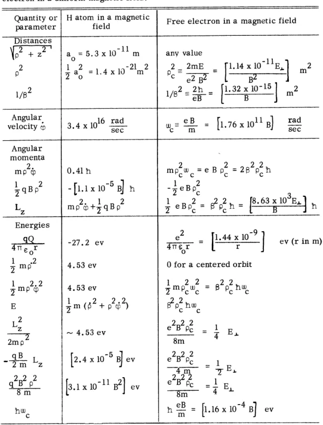
TABLE A1. Numerical estimates of Hamiltonian energies and other quantities of interest, and comparison for the extreme cases of a bound and an unbound electron in a uniform magnetic field.
Quantity or H atom in a magnetic Free electron in a magnetic field parameter field Distances p2 + z a =5.3 x 10⁻¹¹ m any value 2 1 -21 2-21 2 2 2mE 1.14x10 E . p a o =l.4x10 m pc 2 2 =1 B3m2 /2 2 2h _ 1.32 x10⁻¹⁵ 2 1/ 1/ 6 B B m
Angular 16 rad eB [1.76 x 101 B] rad
velocity 3 x sec c m sec
Angular momenta 2. 2 2 22 mp cp 0.41h mpc = e B pc = 28 Pc h 1 2 -5 1 1 2 2 qBp - .xl B h - eBpc 2 1 2 1 2 22 [8.63 x 10³ E Lz mp + qBp 2 eBp Pch c B -27.2 ev 4.53 ev 4.53 ev 1 m (62 -T( + p2 2 ) - 4.53 ev 2.4
I3.1
x
x 10- 5 B] ev 10-11 B 2 1.44 x 10⁹ r 2 e 4TTe r o 22 c 1 S.2-E 1 E, 4 ev (r in m) 0 for a centered orbit1 2 2 222 2.2 2 e B Pc 8m e2B2 2 4m e2B2 2 8m h eB- 1.16 x 10⁻⁴ B] ev Energies qQ 1 -mp.2 2 1 2.2 -mp p E 2 z 2m p qB
-2m
Lz 2B2 8 m hwfor T in degrees Kelvin. Note that (3 is in general a large number compared to unity. For E = 0. 1 eV and B = 0. 1 w/m2 , its value exceeds 103 . A second important parameter for the case of a free electron in a magnetic field is the cyclotron energy iw1c-i(eB/m). Its numerical value is
~tCCL ., X Yx-- e V. (A32)
We shall see that fiw, is the spacing between the levels of the
quantized perpendicular energy EL . For B = 1 w/m2 , a respectable laboratory field, this level spacing is 0. 116 milli-eV.
There are several features about this table which are interest-ing, or will become so in the light of later quantum calculations. We notice first of course that the cyclotron radius is in general much larger than the Bohr orbit radius. Of the two terms which comprise the canonical angular momentum L , the kinetic term for an atom is far larger than the field term qB 2/2 due to the smallness of . For a free electron, on the other hand, these terms are of compar-able size. A further distinction is that L for the atom is of thez order of units of i, whereas Lz for the free electron can reasonably be of the order of thousands of i. Likewise, in the case of the H atom, the energies associated with the magnetic field are negligible compared to the kinetic energies, whereas in the free electron case these energies are comparable. It must be emphasized that the entries are largely estimates and have at best order of magnitude validity. They are intended to encompass the extremes of the dynamical system represented by the Hamiltonian (A22).
A5 The Effect of Coordinate System Rotation Rationale
In the preceding section were considered two limiting cases of the physical system described by the Hamiltonian (A22b). In the
first of these cases we saw that the energy term quadratic in the magnetic field could reasonably be ignored and still leave a term (the energy linear in B) at least partially descriptive of the effects of the magnetic field. This is possible for the charge q in quantum states and magnetic fields such that the energy term proportional
22
to B 2 may be neglected. The Hamiltonian for this limiting case is
- Le
*n 7r .,., (A33)
This Hamiltonian has been studied in connection with the Zeeman effect and the Larmor theorem. General solutions have been ob-tained both classically and quantum-mechanically. The other ex-treme case for which numerical values were given in Table Al
was for Q = 0, that is, the case of cyclotron motion of a free charge in a magnetic field. The Hamiltonian is
+c +. I (A34)
General solutions are of course also known for this dynamical system.
In both of these limiting cases, rotation of the coordinate system brings about considerable simplification in the equations of motion and the solutions. Hence it is natural to employ this tech-nique in attempts at simplification of the equations of motion (A15) through (A17), which may be said to result from the more general Hamiltonian (A22).
Lagrangian-Hamiltonian Formalism in Rotating Cylindrical Coordin-ates
begin by constructing the Lagrangian " from which may be generated the equations of motion referred to a frame rotating with angular velocity n . The prescription is
-
JA
(r-) . (A35)Quantities referred to the rotating frame are starred; Newtonian reference frame quantities are unstarred. The relations necessary to carry out the prescription are given by Symon [1953, p. 240] , among others:
r - (A36)
dt t (A37)
d
1F
d*
--I H-6, (A38)
The first of these equations says that at any given point in time, the position vector as viewed from either system is fundamentally the same entity. That is, at a given point in time, both observers are considering (from the common origin) the same point in space. The remaining two equations relate the behavior of the position vector over intervals of time. They consequently contain terms describing the effects of frame rotation upon observations of the position vector time behavior. Thus the second of the three vector relations states that the Newtonian frame velocity may be resolved into the velocity
as measured by a rotating observer plus the velocity of the rotating frame itself (the Newtonian frame velocity of a point at rest in the rotating system). The Newtonian frame acceleration similarly may be resolved into components associated with the rotating frame.
The first term on the RHS of (A38) is the total acceleration of the position vector as viewed from the rotating frame. The remaining terms give the Newtonian frame components of acceleration due, respectively, to frame rotation (the centripetal acceleration), to motion with respect to the rotating frame (the Coriolis acceleration), and to non-uniform frame rotation.
In what follows, the rotating frame is chosen to be a cylindrical coordinate system rotating about the direction of the magnetic field
= (A39)
The dimensionless parameter E measures the rotation angular velocity in units of qB/m, which for q = e becomes the cyclotron frequency - . We consider that e may vary with time, although, as we shall see, conservation of energy requires that E be constant. Through use of the foregoing prescription, relations, and choice of
y_ , we write the Lagrangian for a particle of charge q and mass m
instantaneously located at r = ( , 4, z) moving in a uniform mag-netic field B = B^ and in the Coulomb field of charge Q fixed at r = ( e , e , z ):
-
z+ (A40)
z*) of the rotating system, and will rely upon the presence of E to indicate that these are coordinates in a rotating frame. This form
and the Newtonian frame Lagrangian are in essential agreement for
6 = 0. There is apparently no choice of e which will completely remove the effects of the magnetic field from this Lagrangian. We note that if the term quadratic in B can be ignored (due either to the small value of the radial distance or the magnetic field, or both), then the choice E = - 1/2 removes all remaining effects of the magnetic field from this Lagrangian. This is the basis of the
Larmor theorem, that the sole effect of the magnetic field upon such a system is a rotation of the system about the field direction at the Larmor frequency eB/2m. The other obvious choice of rotation
speed is E = -1 describing coordinate system rotation at the cyclo-tron frequency. For Q = 0 and a cyclotron orbit centered upon the origin, the particle would be at rest for this choice of E
The canonical momenta are
' (A41)
+ + B (A42)
(A43)
-A YYn
The Hamiltonian, constructed according to the prescription (A21) is
1- -16- 'E>
The Lagrangian Equations of Motion
The Lagrangian equations of motion for the rotating frame are
"" _ ___- - o. (A47)
dt 0 S 04D+ A6
For any value of
ee,
the z equation of motion is unchanged by the rotation (compare A47 with A17). For = 0e 0 (the charge Q situated at the origin), the remaining equations are also invariant. For this location of Q, the canonical angular momentum Lz is conserved as before, and (A46) may be incorporated into (A45) with the result) o. (A48)
The fact that this equation is identical to (A19) does not necessarily imply that the solutions are the same, but only that they are of the same family. It is obvious that for the same physical situation, at least one of the two initial conditions of (A48) would differ from those of (A19). Further, L is not the same constant for (A48) as for (A19). In passing, we note that (A48) is valid also for R,3 0 except that Lz
is then no longer a constant of the motion.
By means of the usual techniques for obtaining energy integrals, the equations of motion (A45) through (A47 may be combined to yield
(A49)
showing explicitly that energy is conserved for constant 6.
We conclude that, for = 0, there exists no value of E which0e will simplify the equations of motion since they remain invariant under coordinate system rotation about the direction of the magnetic field. For e 0, the equations can be somewhat simplified, but
APPENDIX B
SOME FEATURES OF THE CLASSICAL MOTION OF A CHARGED PARTICLE IN A MAGNETIC FIELD B1 Content
In the following appendix, we shall be faced with the assignment of physical meaning to a quantum representation of a single charged particle moving in a magnetic field. In preparation for this inter-pretation, we consider here three constants of the classical motion as well as three other dynamical variables whose time dependence has been removed by averaging over one or more gyroperiods. Of particular interest is the dependence of these quantities upon the cyclo-tron radius and upon the location of the particle gyrocenter with respect to the coordinate system origin. The system considered consists of a particle of mass m and charge q moving in the constant and uniform
A
magnetic field B = Bz.
B2 Coordinates of the Perpendicular Motion
Compared to the motion in the plane normal to the magnetic field, the z motion is relatively uninteresting and quickly may be elim-inated from consideration. In discussing features of the perpendicular motion, we shall utilize the following vectors and coordinates. The particle is Located by the vector 'r extending from the coordinate
system origin to the instantaneous particle position. The plane polar (or cylindrical polar) coordinates of this point are labelled (r, 0). The particle gyrocenter is located by the vector Yro , or equivalently, by the pair (ro, 0 ). The third vector of interest is the cyclotron
radius vector 7' extending from the gyrocenter to the particle. These c
vectors satisfy the equation
r
= r + r . (B l)The associated unit vectors satisfy the relations
x = r e rxc x e (B2)
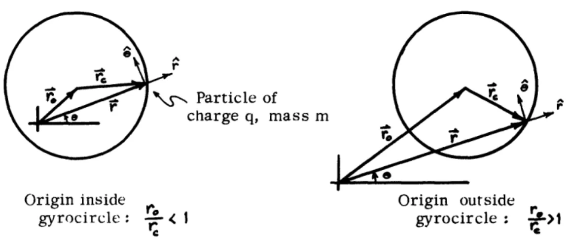
This location scheme and the two cases of interest are illustrated in Fig. Bi. One is the case r /r < 1 when the origin is inside the
oc
gyrocircle; the other is the case ro/rc > 1 when the origin is outside the gyrocircle. There is also the singular, joint case r /r = 1.
o c
B3 Constants of the Motion
There are three basic constants of the motion. One is associated with the motion along the magnetic field and the others with the motion normal to the field. They are the z energy E , the perpendicular energy E_ , and the angular momentum component L (canonical to the coordinate e). Each may be cast into different
z
though equivalent forms:
S_. cos. (B3)
E rL 'Li a3-F
E ' r' sc (B4)
L= (r - Y, )
=
cons+. (B5)That these quantities are constant follows from equations (A16)
through (A18) for Q = O. The expression of the perpendicular quantities in terms of the distances r and r follows from basic vector
defini-o c