COORDINATION OF INVENTORY DISTRIBUTION &
PRICE MARKDOWNS FOR CLEARANCE SALES AT ZARA
By
Orietta Parra Verdugo B.S. Industrial Engineering Arizona State University, 2004
Submitted to the MIT Sloan School of Management and
the MIT Department of Engineering Systems
ARCHVES
in Partial Fulfillment of the Requirements for the Degrees of MASSACHUSETTS INS rTIME OF TECHNOLOGY
Master of Business Administration
AND
JUN 082010
Master of Science in Engineering Systems
LIBRARIES
In conjunction with the Leaders for Global Operations at theMassachusetts Institute of Technology
June 2010
C
2010 Massachusetts InstityA of Technology. All rights reservedSignature of Author
MI Sloan School of Management
epartment of gineering Systems ay 07, 2010 Certified by
C Caplice, Thesis Supervisor Executive Director for the Centev f Transportation and Logistics I-MIT Engineering Systems Certified by
Felipe Caro, Thesis Supervisor Assistant Professor of Decisions, Operations, & Technology Management
UCLA Andcrson .School of Management
Certified by______
C ir6mie Gallien, Thesis Reader Associate essor of Operations Management 1\JIT loan School of Management Accepted by
Nancy Leveson Engineering Systems Division Education Committee Chair Professor of Aeronautics and Astronautics, MIT Engineering Systems Accepted by
Debbie Berechman
Executive Director of MBA Program MIT Sloan School of Management
COORDINATION OF INVENTORY DISTRIBUTION & PRICE MARKDOWNS FOR CLEARANCE SALES AT ZARA
by
Orietta Parra Verdugo
Submitted to the MIT Sloan School of Management and the MIT Department of Engineering Systems on May 07, 2010 in Partial Fulfillment of the
Requirements for the Degrees of Master of Business Administration and Master of Science in Engineering Systems
ABSTRACT
There is an essential need in the retail industry, of integrating inventory planning and pricing strategies. In the fast-fashion world of retail, inventory is treated as a perishable item leading to short selling periods. It is a common practice for retailers to liquidate unsold merchandise via clearance markdown policies. Joint
marketing and production decisions are important and challenging in retailing. Clearance sales depend on the pricing, seasonal effects, and the assortment of goods available to the customer. Errors in inventory
distribution and clearance pricing result in loss of potential revenue or excess inventory to be salvaged. In the case of Spanish-based retailer Zara, thirteen percent of annual revenues are attributed to clearance sales. To maximize these revenues a supply chain tool is designed to facilitate the inventory distribution decisions
for the clearance season while considering price markdowns. A two part linear optimization model considers the demand forecast, pricing decisions, and logistic costs in determining the allocation of excess inventory. The business case is very similar to other retailers where revenues need to be maximized. However, Zara's business model and vertically integrated supply chain makes this case very unique. In a forecast error comparison test, the proposed solution improved the forecast error from 8 to 4 percent in respect to the current forecast process.
Thesis Supervisors:
Chris Caplice, Executive Director for the Center of Transportation and Logistics MIT Department of Engineering Systems
Felipe Caro, Assistant Professor of Decisions, Operations, and Technology Management
UCLA Anderson School of Management Thesis Reader:
Je'remie
Gallien, Associate Professor of Operations ManagementTABLE OF CONTENTS
A b stract... 3
T able of C ontents... 5
L ist of T ables ... 8
L ist of Figures ... 9
A cknow ledgm ents... 10
1 Introduction ... 12
1.1 Overview of Problem Statement ... 13
1.2 Project Methodology ... 14
1.3 Chapter Outline ... 15
2 Company Background... 16
2.1 Sales Campaign and Regular Season... 17
2.2 Organization Team...18
2.3 Product Lines ... 18
2.4 Regular Season Merchandising and Distribution...19
2.5 Clearance Season... 20
3 Clearance Distribution Problem...20
3.1 Legacy Clearance Forecasting...20
3.2 Legacy Clearance Distribution Process...21
3.2.1 Selecting a Reference... 21
3.2.2 C hoosing a Store... 23
3.2.3 Store Shipment Size ... 23
3.3 Proposed Solution... 23
4 Forecasting Model... 24
4.1 Clearance Pricing Forecasting Model... 24
4.2 Regular Season Forecasting ... 25
4.2.1 Forecasting for Weekly Regular Season Sales... 26
4.2.2 Forecasting for the Entire End-of-Season Sales ... 26
4.2.3 Regular Season Comparison Test ... 27
4.3.1 Forecasting Tests for the First Clearance Period... 29
4.3.2 Estimating the Elasticity of Demand ... 30
4.4a ... 34
4.5 Forecasting Process Sum m ary... 35
5 Model Formulation: Clearance Material Distribution Optimization...36
5.1 Model I: Maximizing Revenues Formulation ... 36
5.1.1 Indices and Index Sets ... 37
5.1.2 Param eters ... 37
5.1.3 D ecision V ariables... 39
5.1.4 O bjective Function ... 40
5.1.5 M odel I C onstraints ... 41
5.1.6 L evers ... 44
5.2 Model II: Minimizing Costs Formulation... 45
5.2.1 Indices and Index Sets ... 45
5.2.2 Param eters... 45 5.2.3 D ecision V ariables... 48 5.2.4 O bjective Function ... 48 5.2.5 C onstraints ... 50 5.2.6 L evers ... 51 6 Im plem entation ... 51 6.1 A M PL Files... 51 6.2 M odel I O utput... 52 6.3 M odel II O utput ... 53
6.4 O ptim ization M odel A nalysis ... 53
6.4.1 Legacy Process and Proposed M odel Fit ... 54
6.4.2 W inter 2010 Forecast E rror O verview ... 54
6.4.3 Store Forecast E rror... 57
6.4.4o ... 59
7 C onclusions ... 60
7.1 R ecom m endations for Z ara ... 61
7.2 Future W ork ... 63
8.1 D escriptive Statistics for Forecast Errors ... 64
8.1.1 R egular Season Statistics ... 64
8.1.2 Clearance Season Statistics ... 65
8.1.3 Product Line Statistics... 66
8.2 M odel I A M PL Files... 69
8.2.1 M odel I D ata File ... 69
8.2.2 M odel I Run File ... 71
8.2.3 M odel I M od File... 73
8.3 M odel II A M PL Files ... 76
8.3.1 M odel II D ata File ... 76
8.3.2 M odel II Run File ... 79
8.3.3 M odel II M od File ... 81
9 W ork Cited ... 83
LIST OF TABLES
Table 1: Dem and Forecast Beta-5 Com parison ... 33
Table 2: Rotation Com parison ... 34
Table 3: M odel I Country Detailed Shipm ents ... 53
Table 4: M odel II Store Detailed Shipm ent ... 53
Table 5: M odel II DC Total Shipm ents... 53
Table 6: Legacy vs. M IT Forecast Error ... 57
LIST OF FIGURES
Figure 1: Inventory Distribution...13
Figure 2: Project Overview ... 15
Figure 3: Zara Store in Greece...17
Figure 4: Zara M erchandizing...19
Figure 5: Distribution Center...21
Figure 6: Regular Season Forecast Com parison Test ... 28
Figure 7: Dem and Elasticity Plot...32
Figure 8: Forecast Experim ent Sum m ary ... 35
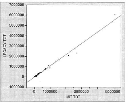
Figure 9: Unit Sales by Country Linear Fit ... 54
Figure 10: Optim ization M odel Descriptive Statistics...55
Figure 11: Legacy Process Descriptive Statistics... 55
Figure 12: Optim ization M odel Capability Analysis ... 56
Figure 13: Legacy Process Capability Analysis ... 56
Figure 14: Legacy Store Descriptive Statistics... 58
Figure 15: Optim ization M odel Store Descriptive Statistics ... 58
Figure 16: Legacy Store Capability Analysis ... 58
Figure 17: Optim ization M odel Store Capability Analysis ... 59
Figure 18: Product Line Unit Sales...60
Figure 19: Group Error Chart ... 60
Figure 20: Optim ization M odel Regular Season Statistics...64
Figure 21: Legacy Regular Season Statistics ... 64
Figure 22: Optim ization M odel Clearance Season Statistics... 65
Figure 23: Legacy Clearance Season Statistics... 65
Figure 24: Product Line A Statistics...66
Figure 25: Product Line B Statistics...66
Figure 26: Product Line C Statistics...67
Figure 27: Product Line D Statistics ... 67
Figure 28: Product Line E Statistics...68
ACKNOWLEDGMENTS
I owe my deepest gratitude to the team at Zara and my advisors for the development and success of this project. I would like to first thank my supervisor, Francisco Babfo, for his continual support, corporate insight, and introduction to the Spanish culture. To Felipe Pefia Pita, who was my right-hand man, for sharing his knowledge and using his curiosity to continuously challenge the
methodologies to grow as a leader. My appreciation goes to Miguel Vinas, Cesar Suarez, and Pepe Corredoira for collaborating on the project and ensuring the outcomes align with current business processes. I would also like to thank Miguel Diaz for being the champion of the project and believing in academia research to continuously improve and grow the organization. To the rest of the Zara family who welcomed me to the organization with open arms and shared their lives, work, and culture with me.
I would like to extend my sincere appreciation to my advisor Professor Felipe Caro who mentored and encouraged me throughout the project. It was an honor working side by side with him and I will forever by grateful. For Professor Jremie Gallien who inspired me take a supply chain adventure in fast fashion. To Professor Chris Caplice for reminding me that business solutions are often practical and simple.
For my family and friends who have helped guide me throughout my life and whose love provides fuel for my soul.
1 Introduction
There is an essential need in the retail industry, of integrating inventory planning and pricing
strategies. In the fast-fashion world of retail, inventory is treated as a perishable item leading to short selling periods in which "inventory and pricing strategies are central to success."' It is a common practice for retailers to liquidate unsold goods via clearance pricing2
. From 1925-1965 average markdowns were stable at 6% but by the mid-1990's they had grown to over 26%3.
The forefront of the problem lies with the demand uncertainty followed by discount decisions made dynamically. Mantrala and Rao (2001), state that in the 1990's there had been an explosion of
product variety on the supply side and consumer tastes had diversified on the demand side increasing demand volatility. With excess inventory on hand, retailers focus on maximizing revenues by
improving clearance markdown policies, which has caused an increase in dynamic pricing strategies in recent years to facilitate these needs4.
Integrating marketing and inventory control was first proposed by Whitin in 1955 and has since received broad attention in the marketing, economics and inventory management literature5. In
1991, for example, Eliasberg and Steinberg designed an integrated joint marketing production decision model. There has also been analysis of pricing strategies in respect to clearance markdowns found in (Gallego & van Ryzin, 1994) as well as (Feng & Gallego, 1995) among others.
The following will discuss a case study on Zara, a Spanish based fast-fashion retailer. It will address a business case, a proposed solution, which will include a demand forecast and a two-part optimization model, and an analysis of the findings with further recommendations. The business case is very similar to other retailers where revenues need to be maximized. However, Zara's business model and vertically integrated supply chain makes this case very unique. The proposed solution suggests a
more sophisticated methodology in coordinating inventory distribution and discount decisions than the current business policy. In a comparison test for forecast accuracy the proposed solution improved the current business process by four percentage points.
1 (Bitran, Caldentey, & Mondschein, 1998)
2 (Wang & Webster, 2009)
3 (Mantrala & Rao, 2001)
4 (Keskinocak & Elmaghraby, 2003)
1.1 Overview of Problem Statement
End-of-season clearance sales is a strategy retailers use to liquidate excess inventory. Each year Inditex S.A. sells less than twenty percent of regular season inventory during clearance sales shown in Figure 1. Within the first seven days, thirty percent of this inventory is sold. Inditex S.A. is one of the largest fashion distributers in the world with revenues of C10.4 billion6. Zara is Inditex's largest
of eight commercial brands and accounts for 65.5% of the total contribution. In 2008, thirteen percent of Zara's revenues were generated during the clearance season. The objective of this project is to maximize clearance profits. In order to facilitate this goal, merchandise should be distributed to
stores with the highest potential of sale and employ the proper discount price.
Clearcce
Regur Price
Figure 1: Inventory Distribution
One of the biggest challenges Zara faces in preparation for the clearance season is determining how to distribute 11,000 different fashion designs to over 1,200 stores worldwide. To accommodate for limited store capacity, shipments of clearance inventory must begin one month before the start of the sale. Once the sale begins, the ability to react and transfer merchandise is limited.
In 2007, Professor Jeremie Gallien, Professor Felipe Caro and Rodolfo Carboni developed a methodology for Zara to determine the price discounts that should be applied to each fashion design during the clearance season7. This model assumed that the physical distribution of the inventory was already at each store. The purpose of this project is to develop a methodology that will optimize store merchandising during the clearance season to later facilitate pricing decisions in which the combination of the two would lead to maximizing revenues. In other words, each store would have
6 (Grupo Inditex 2008 Annual Report)
the right merchandise, at the right time, with the right pricing and gain higher profits during the clearance season.
1.2 Project Methodology
The approach of the project was composed of two parts: determining a demand forecast for end-of-season and clearance end-of-season sales and developing an optimization model prototype that coordinates pricing decisions with store merchandising during the clearance season.
The project began by trying to improve the current clearance pricing demand forecast model developed by Caro and Gallien. This forecast considers the size of the purchase, age, demand rate of the previous period, broken assortment, and price discount as determining factors. The model was adjusted to develop an end-of-season demand forecast. The main adjustment was removing demand elasticity as the price remains steady during the regular season. Next various tests were conducted that determined that the elasticity of demand or the price discount variable was the most sensitive in estimating the demand during the clearance season. Therefore various factors were tested to try to improve the elasticity of demand such as unemployment rate, store to city population ratio, and price demand elasticity of regular season discounts. Though all of these variables and experiments seemed promising, it was concluded that the current model's prediction is the most favorable for both end-of-season and clearance season sales.
Next, two optimization models were developed to determine end-of-season replenishments as well as clearance inventory distribution. The first optimization model used the input from the demand forecasting model to decide how much merchandise to ship to each of the 72 counties to maximize global revenues. Shipment costs from the central distribution centers to each country were taken into account as well as the cost of transshipment between each distribution center. The second optimization model used the output from the first model to disaggregate the country shipments to the store and article level while minimizing costs. In this model, shipment costs to the stores from the distribution centers, country warehouses, and other stores were also considered. The advantages of the model are that it uses a demand forecast, considers discount prices and costs, and determines shipments to a store at a fashion design level. Figure 2 illustrates an overview of the project approach.
-Cearmce duration - Minmums*mentsto coutry cnkd stare -%c3 iwentauyto End of ScasonI De maon d -Sehpn Stoeshipment Clearance V Pead per - Dc to county - Dctoskes shipmentsa CtM e DC-to-DC shipments tm Sa
* Regdcreasan.- storK~eto store
psca pd dg - Warehouseto storew
discounts~saivaUs kM""'"iMri"'
kwuuihe, - DC's, al
- DCs~cuniy warehousesstres -nSb DC'soourh
- CuMnt&NewStores - Sdes&irvvenory
Figure 2: Project Overview
Lastly, a comparison of the current merchandising process with the proposed model will be
discussed. An extensive analysis of the model will be given along with the motivation of the decisions of the proposed model. Recommendations on how to improve the model and how to utilize its methodology in future research will also be discussed.
1.3 Chapter Outline
This thesis is divided into seven chapters as discussed below.
Chapter 2 provides company background and introduces the clearance season and its key
components.
Chapter 3 explains the current forecasting and inventory distribution process for the clearance
Chapter 4 describes the pricing demand forecasting model and outlines the various hypothesis tests conducted to improve and modify the forecast to utilize in inventory planning and pricing decisions.
Chapter 5 outlines the two linear optimization models and its formulations that work in conjunction with a demand forecast to maximize revenues while minimizing shipment costs. Chapter 6 discusses the implementation of the integer programming model in AMPL and the present's the inventory distribution decisions.
Chapter 7 addresses the optimization model's decisions in comparison with the current processes and provides recommendations to improve the model use it in future research.
2
Company Background
In 1975, Amancio Ortega Gaona opened the first Zara store in La Coruna, Spain. Zara provided high quality designer clothing at reasonable prices and quickly gained customer popularity. By 1989, there were 82 stores in Spain with international presence in Portugal, Paris, and New York City. Inditex Group, Zara's parent company, became a publically traded company in 2001 and was the third largest clothing retailer8
. Today, Inditex is the world's largest fast fashion retailer by sales, overtaking GAP Inc. in 2008. Inditex has eight commercial formats including Zara, Pull & Bear, Massimo Dutti, Bershka, Stradivarius, Oysho, Zara Home and its newest brand Uterque. In 2008, Inditex had 89,122 employees in 72 countries with 4,264 stores and over 140 nationalities.
Zara is the flagship chain for Inditex with E6.8 billion in revenues. It is known for its innovative trends in fashion and rapid response to market demand. The key to Zara's success and rapid growth has been due to its virtually integrated supply chain that includes textile sourcing, design, production, distribution and retail. Zara designers look to luxury fashion designers for inspiration for new trends and work together with the fashion savvy regional sales teams to respond to customer demands. The supply chain flexibility, from procurement to distribution, enables new fashion trends to reach stores on a weekly basis. For example, the logistic team is able to take orders from a store and deliver the merchandise within 24 hours for European stores and within 48 hours to American or Asian stores.
8 (Fraiman, Medini, Arrington, & Paris, 2002) 9 (Grupo Inditex 2008 Annual Report)
In the past decade, Zara has grown from 507 stores in 39 countries0 to over 1300 stores in 73 countries tripling its revenues. To thrive with the large expansion, Zara expanded its network of vendors to other European and Asian suppliers. With the rapid growth Zara was forced to rescale their supply chain and improve their current process to maintain their competitive advantage. Figure 3 is a picture of one of the Zara stores located in Greece.
Figure 3: Zara Store in Greece
To facilitate growth strategies, in 2006, Zara began a partnership with the Leaders for Global
Operations (LGO) Program at MIT to develop and incorporate novel forecasting, inventory, pricing and distribution models to their supply chain. Zara stores have three departments Women's, Men's and Kids'. Zara Woman represents sixty percent of Zara's revenues and hence has been selected to pilot new supply chain tools, including those presented here. Past projects with MIT included regular
season replenishment and clearance pricing. The project described here combines merchandising, replenishment and pricing in an optimization that will maximize clearance season revenues.
2.1
Sales Campaign and Regular Season
Zara divides its design collections into two campaigns each year the winter campaign and the
summer campaign. Each campaign lasts approximately six months and at the end of each campaign a clearance season is followed that serves as a transition from one campaign to the next. During the first two weeks of the clearance season the stores position themselves to focus primarily on clearance sales in order to liquidate the old trends. As the clearance season progresses, less and less of the
store s real estate is dedicated to the clearance items. The sale signs in the display windows come down and the new campaign designs are displayed. The clearance season ranges from two to eight weeks and varies in start dates by country and store.
2.2 Organization Team
There are three groups that collaborate to determine the distribution of inventory during the clearance season. The first group is the Performance Management Team (PMT) who estimates the expected sales of each store in both revenues and unit sales. They are responsible for maintaining and updating the store shipment schedule each week.
The second team involved in the inventory distribution process is the distribution group. They forward the schedule of shipments to the distribution centers (DC) to create work orders. Because the schedule specifies number of units for each store it is up to the DC to pick and choose the stock keeping units (SKUs) to distribute to each store. A SKU is a particular size and color of an article.
Lastly, commercial managers are responsible for store sales and are the market experts in the countries and regions they manage. They are in contact with store managers on a daily basis and have familiarity with store inventory needs. Once the schedule of shipments is released, they work with the PMT and the distribution group to make any adjustments to the schedule. Commercial managers can also block shipments of certain trends to a given region. A common example is blocking the distribution of heavy coats to the Middle East during the summer months. Due to hot weather conditions, customers are less likely to buy coats even at a discounted price.
2.3 Product Lines
The Women's Department is separated into six product lines that have a team of designers and buyers who are responsible for the quality and success of the designs. The product lines vary in price, design, and fit. Some for example have more trendy designs while others have basic trends for casual use. Within each product line there are groups that further categorize each segment such as dresses or pants. In each group there are references or articles, which are design trends that are categorized by a model and textile quality. For example, a reference such as a denim jacket would be under the outerwear group for product line A.
2.4 Regular Season Merchandising and Distribution
Merchandising decisions are essentially investment decisions made by retail managers". From a marketing prospective, there are many advantages to offering a wide assortment of products. Van Ryzin and Mahajan suggest that having such an assortment will increase the likelihood a customer will purchase something from that assortment (1999). Merchandising is centralized at Zara from inventory distribution to store merchandising.
During the regular season, Zara's inventory distribution philosophy uses a forecast to predict the following week's sales based on historic sales. A demand forecast and optimization model created by Gallien and Caro is used to maximize revenue for a reference and determines how to allocate the inventory to each store . Zara's information technology system also enables store managers to place any additional merchandise orders from a personal digital assistant (PDA). m
Figure 4: Zara Merchandizing
Store merchandising is fundamental to Zara's unique customer experience. At headquarters, Zara has mock stores where visual merchandisers design store layouts including window and in-store displays as well as a design assortment to facilitate a standard Zara appearance worldwide. Store dynamics includes a very detailed process to ensure a well assorted collection of fashion designs shown in Figure 4. This includes a strict rule on the number of sizes that can be displayed at a time for a given article and a quick replenishment process once an item is sold.
11 (Sweeney, 1973)
2.5 Clearance Season
Zara approached Professors Gallien and Caro to assist them once again in an optimization model but this time for clearance season sales. The approach taken by the professors was to develop a two-step process. The first was to establish a pricing policy to ensure articles during the clearance season were priced in a manner that maximized revenues. Zara's current pricing policy is managed by the Pricing Team and country managers. Each week during the clearance season the sales team reviews its sales at the current price and based on experience and instinct make pricing decisions. In 2007, LGO Rodolfo Carboni in conjunction with Gallien and Caro worked on an optimization model that would facilitate the pricing decisions".
The second step, which will be discussed here, is ensuring stores receive the proper merchandise for the clearance season. The combination of having stores with the right merchandise and priced at the right levels would facilitate Zara's goal of maximizing clearance revenues. Similar methodologies are used in both projects purposely in order to facilitate integration.
3 Clearance Distribution Problem
One month before the start of the clearance sale the Performance Management Team estimates store sales for the remainder of the regular season merchandise. This includes sales from both the last month of regular season and those accumulated from the clearance season. With this estimate a store shipment schedule is created and is used by the business as the main distribution plan. This chapter discusses the clearance season in more detail focusing on the current inventory distribution decision process. The process includes the existing clearance forecasting method as well as the allocation of goods to each store.
3.1 Legacy Clearance Forecasting
The current forecasting method used by the PMT is based on data from similar campaigns and seasons. Therefore, when estimating sales for the current winter clearance season the previous year's winter clearance sales data is used. The forecast is calculated by taking into account the sales from the previous year and the current sales trend for that campaign and season. These estimations are in both revenues and unit sales.
The forecasting method ensures all merchandise in the DC's is distributed to the stores. Therefore, stores are expected to make an effort to sell the excess inventory. A load factor that proportionately allocates the inventory is used to calculate the expected effort of the store. The load factor
considers the inventory levels in the network including country warehouse, distribution centers, and stores. If there is sufficient inventory in the store to cover the estimated sales, the store will be blocked from additional shipments. Once the store estimations are complete they are aggregated
at a country level to identify if a country needs to be blocked.
The forecast drives the store shipment schedule by determining total store sales. The shipment schedule uses this information to breaks down the total shipment by weekly shipments. Weekly shipments are derived by a combination of store inventory capacity and maximum shipment levels.
3.2 Legacy Clearance Distribution Process
The PMT manages a schedule of shipments that is sent to the distribution center to decide what merchandise each store will receive. A three step process is used by the distribution center to determine the shipments. These steps are first selecting a reference, determining which stores to ship the reference, and calculating the shipment size.
Figure 5: Distribution Center
3.2.1 Selecting a Reference
The first step is selecting a reference to distribute. Zara's picking system is based on inputting a reference and then assigning the quantity to ship to all stores. DC personnel pick at a reference level
and then the item is physically sorted by store. This is different than picking a set of references for a given store.
To choose which reference r , the distribution team considers merchandise with the highest success ratio, lowest stock to sales ratio, and most inventories. Each reference has a success ratio
SSr , which
is the ratio of total sales of a reference divided by the total opportunity of sales for the currentseason. This estimates the success of sales over the life of the item. The range of the success ratio is from 0 to 1 and used as a percentage of inventories that has been sold at a given store. A success ratio of 0.8 signifies that 80 percent of the total inventory available to the store has been sold. Equation 3-1 describes the success ratio in which
Inventoryr
is the current stock on hand at a given store andSales,
is the total sales of that reference.s
= Sales
.
Invenotry,. + Sales r
Equation 3-1: Success RatioNext, references are sorted by those with a low stock to sales ratio. The stock to sale ratio or rotation
Rot,
is "a direct index of the stock which should be on hand at each store in a given time.1 4" Itdivides the stock at the end of a period with the sales during that period. Rotation is the number of days the current inventory will remain on hand at a store if the sales rate remains the same for that period. This differs from the success ratio as it is only captured at a given period and not the entire season. At Zara, the stock to sales ratio is estimated on a daily or weekly basis. Equation 3-2 is the rotation calculation for a given period.
Inventory Rot -
Sales
'Equation 3-2: Rotation
By considering the success ratio
SS,
and the stock to sale ratioRot,
the DC is ultimately choosing to ship those items that are selling very well first. The sooner these items are in the store the more likely they will be sold during the first week of clearance and will not have to be discounted numerous times.Lastly, references with the most inventory on hand take priority shipment. Items with the most stock on hand are those that did not have success during the regular season. If there is an excess amount of these items in the distribution centers they are likely to be used to fill store orders due to the volume of the merchandise.
3.2.2 Choosing a Store
To choose which stores should receive a shipment of a chosen reference, the DC team considers first those stores that have the highest total unit sales of the reference and the highest sales of that reference the previous week. The information system, based on point-of-sale, has this information easily accessible for the user to monitor. Stores that have been blocked by the commercial manager will have an alert in the system and will not allow the user to assign a pick list to that store. A final method of choosing a store is based on the DC's knowledge of that market. For instance, if the reference is a pair of Bermuda shorts and it is known that historically Japan sells many Bermudas, Japanese stores will have a priority of these shipments with respect to another country.
3.2.3 Store Shipment Size
The size of the shipment to each store is based on the current inventory level of that store and its sales the previous week. Conventionally store shipments are larger for the clearance season than for the regular season since the merchandise is to replenish stock for the entire clearance season and not just one week of sales. If there is an item in which there are less than a few thousand articles
available, the DC will ship to only those few stores with the highest historical sales. Once the top references have been evaluated and assigned to a store the team sums the total shipments quantity per store. A report is printed out with each stores shipment size and compared to the schedule created by the PMT team to ensure the proper shipment sizes are implemented.
3.3 Proposed Solution
The proposed solution to this process is to create a demand forecast that will be use to determine sales for both end-of-season and clearance season. It will be an automated process in which point-of-sale data would be used for inventory and past sale records, making the forecast more viable. An optimization model based from linear programming will be implemented to make distribution decisions for each reference by maximizing profits for the global network and then minimizing costs for distribution within each country.
4 Forecasting Model
The fashion industry relies heavily on sales forecasting for operational decisions. Demand is very volatile and "any gaps between supply and demand leave stores holding too much of what customers don't want and too little of what they do"15. In Chapter 3 the traditional forecasting tools used by Zara and how historical data is used to reflect current trends are discussed.
In this chapter the current forecasting model created by Caro and Gallien in 2007 is addressed. This model that will be referred to as the pricing forecast, considers five variables to estimate demand including the elasticity of demand in each country. It encompasses data from both the current
season as well as historical sales from the previous two years. Next, the model is analyzed by running various simulations and hypothesis testing to determine key decision variables to improve forecasting accuracy. Finally, a forecasting model for end-of-season demand is formulated.
4.1 Clearance Pricing Forecasting Model
In 2007, Caro and Gallien developed a forecast to estimate demand of a given reference at different price points during the clearance season. The pricing forecast estimates expected unit sales for a given reference at a group and country level. In Carboni's case study, he found that the sales data was most accurate when observed at an aggregated reference level. The pricing forecast is described
in Equation 4-1.
[4 LN MIN 1 InvPos ' Y sLN
, * (Q*LN (Purchase,)* (i62Age,) * e(pLN(A)) * jLf *C, *S,. pJ
Equation 4-1: Pricing Forecast16
There are five explanatory variables, purchase, age, demand level, broken assortment, and price discount. Purchase represents the global purchase in units of the given reference. Age refers to the number of days the reference has been in the store starting from the day it shipped out of the distribution center. The demand level is an estimation of demand based on sales from the week before. Broken assortment refers to the variety colors and sizes available for a given reference. Finally, the price discount is the price elasticity of demand also referred as
p
15 (Friend & Walker, 2001) 16 (Carboni, 2008)
Regular season data is used to calculate
#lo
(the intercept) through 63 (demand level) in a minimum squared error linear regression. In order to normalize the regression, the model removes the effects of seasonality and product assortment by using intra-week (delta) and inter-week seasonality. Intra-week refers to seasonality observed from one day of the Intra-week to the next. Inter-Intra-week seasonality measures sales patterns from one week in the regular season to another.The broken assortment
($4)
and price discount(#5
) is calculated using historical regular season and clearance season data. In order to estimate the price elasticity of demand, past data is important when capturing the price sensitivity of each reference by country. the broken assortment also changes during the clearance season as the majority of the reference collection was sold during the regular season. 84 and#5
are calculated through a series of residuals and then are fitted in the linear regression with the other variables.Once the demand forecast is calculated it is must be converted into unit sales. The demand is than multiplied by an alpha parameter that disaggregates the demand to a color, size, and store level. Currently the demand is at a reference by country level. Next, it is multiplied by the delta intra-week seasonality that gives an estimated demand by the number of days of the clearance period. During the clearance season, each period of sales may vary in number of days as it is dependent on when the business decides to make a pricing decision. Finally, the Gamma Distribution is used to convert this calculation into unit sales.
4.2 Regular Season Forecasting
The pricing forecast created by Caro and Gallien estimates clearance sales using both historical and current season data. Conceptually, the fitted model should be able to predict regular season demand by using
#le
through164.
In this section this hypothesis is tested by predicting one week in the regular season and then using the model to estimate sales for the remainder of the regular season. As mentioned in Section 3.1, the current forecast is calculated four weeks before the clearance season. In order to allow decision flexibility the forecast analysis in this chapter is based on an eight week horizon.Belgium's winter 2008 regular season data was used to test the model. Belgium was chosen as it is a medium size country with 25 stores and has been the pilot country chosen by Zara. The broken assortment parameter will be calculated with the regular season data through the linear regression.
Historical data will not be used as the price discount parameter will not be incorporated since there is no change in prices during the regular season.
4.2.1 Forecasting for Weekly Regular Season Sales
The first test conducted was to understand if the pricing model, with modifications, would predict weekly sales during the regular season. Meaning, can the pricing model determine sales for week t+1 with current regular season data through week t. Modifications to the pricing demand model were calculating 84 with regular season data and removing
#5
. Another alteration needed for the model was to use seven days for the delta intra-week seasonality used to transform the demand to sales. Seven days represents the duration of a regular season sales week.The sales forecast in comparison with the true sales resulted in a forecasting error of -1 percent. With such a low error it was concluded that the modified forecast gave an acceptable estimation of weekly sales. However, it was unclear if the model could estimate the eight weeks leading up to the
clearance sales. This is imperative to have when making the inventory distribution choices.
4.2.2 Forecasting for the Entire End-of-Season Sales
To determine if the same approach could be used to estimate the last eight weeks of the regular season two methodologies were tested to calculate the intra-week seasonality. The first approach was a straight line estimation using 56 days (7 days x 8 weeks) as it represents the remaining days left before the clearance period. The second approach was a calculation based on the number of days a SKU was on display at each store. In this latter method, it took the average days a given color and size of a reference was on display per store. The number of days was calculated based on the day of the first shipment to the store.
Though the average number of days on display of a SKU appeared to be logical, when testing both methods this approach gave a large underestimation compared to the straight line approach. There were many doubts about the straight line approach as sales tend to drop as the regular season comes to an end. The results however proved to give a feasible prediction for two months in the future. The new regular season forecast is shown in Equation 4-2. This equation is the same as Equation 4-1: Pricing Forecast but does not contain the price discount (p8 ) variable.
(8 , * * (.. ,Age')( )) * LN MIN 1, InvPos "'
e ( LN(Purchase)) (62 A e (3LN(, *e ' f *C,*S ,
Equation 4-2: Regular Season Forecast
4.2.3 Regular Season Comparison Test
After testing the regular season forecast, it was compared to the legacy forecasting method discussed in Section 3.1. In the legacy method, the forecasts are estimated at a store level. The regular season
forecast, on the other hand, is based on sales for a reference therefore this estimation was
disaggregated to a store level in order to compare both techniques. The forecast error is calculated by taking the difference between the forecast and the actual sales and dividing by the actual sales as
shown in Equation 4-3.
Forecast Error = Forecast - True __Sales
True Sales Equation 4-3: Forecast Error
Figure 6 shows the forecast error of both methods for each Belgian store. A negative error represents an underestimation of the forecast where a positive error represents an overestimation. From a store level there is more variation in the forecast error using the regular season forecast. However, at the aggregated country level, the regular season forecast gives a closer estimation of sales than the legacy method. The ideal forecast the organization would like to obtain would be one that decreases both store and country variation.
337 -10% 6% 339 -5% -1% 340 -a% -10% 346 -7% 12% 348 -1% 5% 376 -11% 9% 377 -20% 2% 378 -4% 6% 388 -8% -4
392 -
Belgium-W08
Old
New
3014 244 6% 3139
-12%1 -18%
'-I
Totai
-8%
-1%
3141 -15% -19% 3168 -9% 95 3193 - A% 3295 -12% -10% 3332 - % 3542 -5% 3578 101% 73% 3589 -6% 10% 3597 -1%0 0% 36P1 -10% 17% ---Figure 6: Regular Season Forecast Comparison Test
With the regular season trials, the team was comfortable with the formulation of the regular season forecast and the results of the comparison test. The next step was to focus on estimating sales for the clearance season followed by experimenting with adding additional variables to improve the demand forecast.
4.3 Clearance Season Forecasting
The pricing forecast is based on all data leading up to the clearance season. In other words, it captures the entire regular season information to estimate clearance sales. Smith and Achabal's
(1998) research demonstrates that the first clearance markdown tends to be the dominant
decision economically. With this in mind, Caro and Gallien designed the pricing forecast model to estimate the first period of the clearance season and through a pricing optimization model to calculate the total clearance sales".
The following tests focus on improving the first period of the clearance season by using the pricing forecast. The first experiment was to test the forecast error using the data that would be available eight weeks prior to the start of the clearance season. The second experiment was testing other variables that may affect the elasticity of demand for the pricing discounts.
4.3.1 Forecasting Tests for the First Clearance Period
Estimating clearance sales two months before the sales begin is challenging. One aspect to consider is that the inventory position in the current period will be different once the clearance season begins. The current inventory position changes as there will be both sales and merchandise replenishment in the eight weeks leading up to the clearance season, both of which are unknown. Inventory position affects the calculation of the broken assortment variable in the linear regression. Moreover, it impacts the conversion of the demand to sales through the Gamma Distribution. The Gamma Distribution has two parameters k and theta. Theta is the scale parameter and in the Caro and Gallien pricing model is the demand multiplied by the intra-week delta factor and an alpha that disaggregates the reference to a SKU and store level. Current stock level or inventory position is the parameter k used to shape the Gamma Distribution. Changes to the stock level will impact the sale estimation. Various iterations of the inventory position were tested to analyze how feasible it would be to estimate the first week of clearance sales.
In this analysis winter 2008 data for all stores in Belgium were used. The clearance period duration for the winter 2008 was five days, therefore the intra-week seasonality resulted in a 4.8 value18. This of course is an after-the-fact data point but was used to understand the viability of the model. The various inventory positions are described below:
e Inventory Position I: The inventory position eight weeks prior to the start of the clearance season, this would reflect the stock levels the business can identify.
* Inventory Position II: The stock level eight weeks prior to the clearance period plus all shipments within the eight weeks. In practice an estimation of all the shipments would not be feasible but was tested to determine the significance of these shipments.
* Inventory Position III: The inventory position at the start of the clearance season. The inventory level at the beginning of the clearance season would be unknown in practice as both shipments and generated sales would have to be considered.
The experiments showed that there was little difference with the forecast errors when using
Inventory Position I versus Inventory Position III. The second inventory position did not offer any convincing insights and was quickly discarded. It was concluded that using stock levels two months
prior to the clearance season provides a demand forecast similar to one when knowing the true stock level at the start of the clearance season. Consequently the pricing forecast could be used to
determine the first period of the clearance season given a shortage on regular season data. 4.3.2 Estimating the Elasticity of Demand
Price elasticity of demand is "a measure of the sensitivity of quantity demanded to changes in price"19. The current model estimates the elasticity as a function of historical sales in the previous two years. However, it fails to test if there are external factors that can influence the ratio between quantity demanded and change in price. For the following experiment three years worth of data (2006-2008) for the summer clearance season was used to test the variables for 10 countries using a linear regression approach. The next section describes the factors considered as viable variables to test.
4.3.2.1 Test Variables
1) Country Growth Domestic Product rate year over year20: GDP was used to understand if
there was a trend with a countries growth that it may affect the elasticity of demand.
2) Country unemployment rate year over year": Unemployment rate was considered due to the social impacts and changes in spending trends in consumers.
3) Store to city population ratio22: The ratio of population of each city to the number of stores in each country was considered to understand the dynamics of any cannibalization between stores.
4) Country economic position: Economic position of a country was a measure of how many hours a store employee would have to work to be able to purchase an article from the store. 5) Regular Season Markdowns: The price elasticity of demand of regular season mark
downs.
19 (Wikipedia Elasticity of Demand)
20 (European Commission Eurostat) 21 (European Commission Eurostat) 22 (City Population, )
4.3.2.2 Elasticity of Demand Regression Analysis
The pricing forecast focuses on estimating sales for each of the 21 groups at a time. As mentioned in Section 2.3, groups are categorized into product lines. Through analyzing historical sales, there was evidence in trends amongst product lines. Therefore, the elasticity of demand was estimated at the product line level. Using the true
#5
for the summer clearance season, the elasticity of demand for the product line was calculated by taking the average /, of the groups within the product line. To test the correlation of the variables with the elasticity of demand, three years worth of data was used for 10 countries with a total sample size of 30 per product line. The linear regression tested each of the variables independently with only unemployment rate and regular season markdowns proving to be statistically significant. The relationship with unemployment rate and the elasticity of demand signified that consumers were more sensitive to price mark downs as the unemployment rate inceased. However, using unemployment rates to determine the elasticity of demand for theclearance sales has its short comings as these figures may not be readily accessible for all countries. The elasticity of demand from the regular season markdowns, on the other hand, is a more practical
solution. The next step was to test the theory by estimating the elasticity of demand using current season data.
4.3.2.3 Estimating,5 with Regular Season Markdowns
The plot of the linear regression using three years worth of data can be found in Figure 7. The dependent variable
#8
product line was estimated by taking the weighted average elasticity of each group within the product line. Markdown elasticity was measured using the definition of priceelasticity found in Equation 4-4 were D is unit sales and Pis price. Since the unit sales are known for the price markdown during the regular season, demand was not necessary.
AD/D Elasticity= AP/P
AP /P Equation 4-4: Markdown Elasticity23
The change in sales was determined by the sales of the last seven days at the regular season price denoted by variable e and the sales for the first seven days at the markdown price denoted by variable
b . The price ratio was calculated by using a weighted average that was dependent on the inventory volume for each reference r. Equation 4-5 and Equation 4-6 illustrate the sales and price ratio
respectively.
AD/D = (Db-De) De Equation 4-5: Change in Sales Ratio
Stock, * e)__
1 Stock,
Equation 4-6: Change in Price Ratio
To estimate the elasticity of demand for summer 2009, a simple linear regression was used given by the regression analysis of the historical data. The relationship between the two variables can be found in Figure 7 wherey is the
#5
product line for 2009 and x is the markdown elasticity for 2009.Relationship of Historic Elasticity
0- -0.5- -1- -1.5- -2--2.5 - -3- -3.5-r--14 , I I , , -12 -10 -8 -6 -4 Markdown Elasticity -2
Figure 7: Demand Elasticity Plot
This linear relationship will give the elasticity of demand at the product line level, therefore needs to be disaggregated at a group level for the pricing forecast. To estimate the
#5
group (B5G we took the weighted average from the previous year as denoted in Equation 4-7. Where B5pL representsp5
product line and tis the current year.* y = 0.217x - 0.059
B5
t'
B5
t'-
GB5
Equation 4-7: Beta-5 Weighted Average
Equation 4-8 portrays the final calculation of B5G by multiplying the group weighted average by
B5PL.
B5' = B5'L *B5 t-1
Equation 4-8: Beta-5 Group Estimation
With the estimated
#5
for summer 2009, the pricing forecast was tested with these new values versus the values given though the residual analysis discussed in Section 4.1.Next, 10 countries with regular season data up to two months prior to the clearance season was used to test the pricing forecast. The forecast errors using both methods of calculating the elasticity of demand were compared and are shown in Table 1.
-4% -11% -8% -23% -3% -10% -4% 11% -2% -12% -2% 1% -26% -41% -3% 23% -21% -22% 25% -22%
Table 1: Demand Forecast Beta-5 Comparison
The results showed that estimating the
,6
using regular season markdowns improved the pricing forecast by an absolute error in country 28 and 101. However, the pricing forecast overall had a smaller error percentage for 80 percent of the countries tested. Another insight from this test was that the model was successful in terms of forecast error for multiple countries not just one as tested in Section 4.3.1.4.4
New Variables for Demand
The last hypothesis in improving the pricing forecast was to determine if adding an additional variable to the current five variable pricing forecast would decrease the overall forecasting error. In
Section 3.2.1 the stock to sales ratio called rotation was discussed as a factor that Zara uses to
measure how well a given article is performing. A rotation of 5 signifies that the current inventory for a reference would last 5 days if the store continues to sell at that rate. The data used in this
experiment was winter 2008 figures for three medium size countries. To test if the Rotation variable was significant in determining demand, it was added to the linear regression as
$6
and calculatedusing regular season data. Given that the rotation is the stock to sales ratio, there are various techniques that can measure this variable. Therefore, three distinct rotation measurements were tested by adding them to the regular season forecast and the pricing forecast. Below are the rotation calculations and results of these experiments.
1. Rotation of the first day of sale 2. Rotation of the first week of sale 3. Rotation of the total regular season
Collecting the data for the first two rotations was a tedious task as each article had its individual first day of sale. The third rotation measurement took less effort to collect and calculate as it was the ratio of the sum of total inventory and total sales for the regular season. Table 2 is a comparison of each rotation measurement for a sample reference.
First Day of Sale 4.35 First Week of Sale 3.81 Total Season Sale 4.12
Table 2: Rotation Comparison
The rotation tests were tested on both the regular season forecast and the pricing forecast. In each case, the results were not compelling. In the case of the pricing forecast, all three rotation
calculations were not statistically significant in the linear regression. The third rotation calculation, however, was statistically significant in the regular season linear regression. The sales estimation for
method but was not the case in comparison to the regular season forecast as shown in Equation 4-2. It was therefore concluded that rotation is not a significant variable and will not be added to the two forecasting methods.
4.5 Forecasting Process Summary
Caro and Gallien's pricing forecast proved to be sufficient in determining both regular season sales and clearance season sales with limited data. The forecast is aggregated at each reference and predictions are arranged at a group and country level. A linear regression analysis is used to determine demand and finally converted to sales though the Gamma Distribution.
The regular season forecast is a modification of the pricing forecast in that it did not contain the price discount variable. A straight line estimation approach was used to estimate the sales for the ending weeks of the regular season. The demand forecast is then converted to a sales forecast for the optimization models discussed in Chapter 1.
H1:Pridng forecast can predict regularsen sales.
1 a Intra-week delta= Straight line rnthod
* Intra-week delta =Days on display
ExtBenui factDEs dCt priCe elatlC nli can mpnuve prldngforecast.
1 External factors can predict beta-5
* Regular season rnarkdowns
i
e
Unernployrnent
rate* Country GDP
- Store to city population . e country economic position
2 Regular~ussan narkdmns mpoefre cast
*
:Adg PAtation as a varale will improve forecast.1
eRotation=
Firsitdayo saleRua Rotation= First week of sale * Rotation= Total season sale
Figure 8: Forecast Experiment Summary
In estimating demand for the clearance season, the pricing forecast proved to be sufficient. Various tests were conducted to improve the model as shown in Figure 8 but all failed in providing
compelling evidence to change the current model. The demand for the first week of the clearance season at various discounted prices is determined by using the pricing forecast and an optimization
model discussed in Carboni's case study. To estimate inventory distribution for the clearance season, a demand estimate is used for the clearance season rather than a sales estimate as used in the regular season forecast. This is due to the optimization models that will be discussed in the following chapter that will determine the shipment based on the available inventory and demand.
5
Model Formulation: Clearance Material Distribution Optimization
The optimization model was broken down into two models in order to be able to manage the size of the data of 11,000 SKUs and 73 countries. The objective of the first model is to maximize global profits for each group and pricing cluster by determining the allocation of inventory to each country. A pricing cluster is a set of references that have the same regular season price. It uses the demand forecast at each of the various price points from the regular season price to the distinct price discounts during the clearance season. The output of this model will be the number of units to ship to a county in a given group and pricing cluster. In the second model it will take each group and cluster and allocate these at a reference level to each store while minimizing shipping costs. With this model users can determine what reference to ship to each store from the distribution centers and local warehouses as well as which
references to transfer from one store to another. These two models are designed to run a few weeks before the clearance season begins to assign the total number of units by reference to ship to each store for both end-of-season and clearance season sales. The two models were formulated by Professor Felipe Caro2 4
.
In order to distinguish the variables between regular season and clearance season, in the
following section variables and parameters with a tilde - will denote regular season. For example Fm, and Fg,, denote the sales forecast for a given country m , group g, and cluster n during the regular season and the clearance season respectfully.
5.1
Model I: Maximizing Revenues Formulation
The purpose of this optimization model is to maximize global profits by making inventory distribution decisions based on a dynamic pricing system. The model considers each product
24 (Caro F. , In preparation for: Coordination of Inventory Distribution and Price Markdowns for Clearance Sales, 2009,
group and pricing cluster in determining the allocation of the inventory to each country. Inventory and demand estimates are taken from the POS system each period for data accuracy. For clearance markdowns it is assumed that pricing decisions are permanent, therefore cannot increase overtime. The general notations of the model will be introduced first followed by the definition of the parameters.
5.1.1 Indices and Index Sets
e m e M: Each county within the distribution network. The index m will also be used to denote local warehouses for those countries in which it exists.
e a e
A:
Main distribution centers located in Spain. Thus, a(m) denotes the distribution center that supplies country m and a(j) the distribution center that supplies store j. LetP(a) C
M
andT(a)
q J denote the set of countries and stores respectfully that are supplied by the distribution centers.* g
e
G: Clearance sales groups that represent each product line and are numbered from 1 to 21.* n E
N(g):
Price clusters in a given group g. each group g has distinct price clusters thatrepresent several references r .
*
k
eK
={k:
k
>
1: Clearance prices are indexed by (k). Let Pk denote the set of clearance prices that increases by convention, i.e. p P2 --- Pk, where p, is the final liquidationpnce.
" w e
W
={w:
0W
<W}:
Periods within the clearance season, where w = 0 represents thefirst period of the clearance season and w = W the last period of the season. 5.1.2 Parameters
Each country has different price clusters based on their currency as well as their local market demand. For example, an article in the distribution center may be categorized in price cluster 9.99 Euros. That same article in a different country might have a different price point in the local country currency. In order to allocate the inventory the clusters were standardized in the pricing categories