Comparing Different Methods to Create a Linear Model for Uncontrolled Manifold Analysis

(1)

HAL Id: hal-02185115

https://hal-amu.archives-ouvertes.fr/hal-02185115

Submitted on 16 Jul 2019

HAL is a multi-disciplinary open access archive for the deposit and dissemination of sci-entific research documents, whether they are pub-lished or not. The documents may come from teaching and research institutions in France or abroad, or from public or private research centers.

L’archive ouverte pluridisciplinaire HAL, est destinée au dépôt et à la diffusion de documents scientifiques de niveau recherche, publiés ou non, émanant des établissements d’enseignement et de recherche français ou étrangers, des laboratoires publics ou privés.

for Uncontrolled Manifold Analysis

Inge Tuitert, Tim Valk, Egbert Otten, Laura Golenia, Raoul Bongers

To cite this version:

Inge Tuitert, Tim Valk, Egbert Otten, Laura Golenia, Raoul Bongers. Comparing Different Methods to Create a Linear Model for Uncontrolled Manifold Analysis. Motor Control, Human Kinetics, 2019, 23 (2), pp.189-204. �10.1123/mc.2017-0061�. �hal-02185115�

(2)

Comparing Different Methods

to Create a Linear Model for Uncontrolled

Manifold Analysis

Inge Tuitert

Aix-Marseille University and University of Groningen

Tim A. Valk, Egbert Otten, Laura Golenia, and Raoul M. Bongers

University of Groningen

An essential step in uncontrolled manifold analysis is creating a linear model that relates changes in elemental variables to changes in performance variables. Such linear models are usually created by means of an analytical method. However, a multiple regression analysis is also suggested. Whereas the analytical method includes only averages of joint angles, the regression method uses the distribution of all joint angles. We examined whether the latter model is more suitable to describe manual reaching movements. The relation between estimated and measured ﬁngertip-position deviations from the mean of individual trials, the relation betweenﬁngertip variability and nonequivalent variability, goal-equivalent variability, and nongoal-goal-equivalent variability indicated that the linear model created with the regression method gives a more accurate description of the reaching data. Therefore, we suggest the usage of the regression method to create the linear model for uncontrolled manifold analysis in tasks that require the approximation of the linear model.

Keywords: Jacobian, motor control, uncontrolled manifold method

The uncontrolled manifold (UCM) method is a well-established approach to assessing the coordination of multiple degrees of freedom (DoF) in synergies that stabilize performance in human actions. The method has been applied to a variety of actions, such as sit-to-stance,ﬁnger-force production, and goal-directed reaching (Black, Smith, Wu, & Ulrich, 2007; Domkin, Laczko, Djupsjöbacka, Jaric, & Latash, 2005; Greve, Zijlstra, Hortobágyi, & Bongers, 2013; Klous,

Tuitert is with Aix-Marseille University, CNRS, Institut des Sciences du Mouvement, Marseille, France. Tuitert, Valk, Otten, Golenia, and Bongers are with the University of Groningen, University Medical Center Groningen, Center for Human Movement Sciences, Groningen, the Netherlands. Address author correspondence to Inge Tuitert [email protected].

(3)

Danna-dos-Santos, & Latash, 2010;Krüger, Borbély, Eggert, & Straube, 2012;

Romero, Kallen, Riley, & Richardson, 2015;Scholz, Schöner, & Latash, 2000;

Shim, Hsu, Karol, & Hurley, 2008;Togo, Kagawa, & Uno, 2016;Van Der Steen & Bongers, 2011;Wu, Pazin, Zatsiorsky, & Latash, 2012;Yang, Scholz, & Latash, 2007). The current paper focuses on computational aspects of the UCM method in goal-directed manual reaching movements to illustrate the argument. When performing a reaching movement, the DoF, that is, the joint angles of the arm, have to be coordinated to stabilize the index-finger position. To assess how the joint angles are coordinated, the UCM method is applied to evaluate the variability in the joint angles across trials. Joint-angle variability is partitioned into variability that does not influence the index-finger position (goal-equivalent variability, GEV) and variability that does (nongoal-equivalent variability, NGEV). If there is more GEV than NGEV, it is assumed that the joint angles of the arm are coordinated into a synergy that stabilizes the index-finger position.

The computation of GEV and NGEV with the UCM method requires four steps (Latash, Scholz, & Schöner, 2007). Thefirst two steps consist of selecting the elemental variables and the performance variable, respectively. In goal-directed manual reaching, elemental variables are usually the nine joint angles of the arm (shoulder, elbow, wrist, andfinger-joint angles) while the 3D position of the tip of the indexfinger is the performance variable. Subsequently, small changes in the joint angles are related to small changes in the index-finger position by means of a linear model (third step). These relations have to be approximated in goal-directed manual reaching movements and are represented in a Jacobian matrix. Lastly, this matrix is used to partition the joint-angle variability across trials. Variability within the null-space of the Jacobian corresponds to GEV, and variability orthogonal to the null-space corresponds to NGEV. The current paper focuses on the creation of a linear model, which can be done either by means of an analytical method or by means of multiple regression (see below). Although the analytical method (Scholz & Schöner, 1999) is the most often used of the two (de Freitas & Scholz, 2010), the regression method uses more data to create the linear model, which can influence the accuracy with which the model describes the data. In this paper, we compare the accuracy of the two methods in a manual reaching task.

In reaching movements, the analytical method to create the linear model (de Freitas & Scholz, 2010;Scholz & Schöner, 1999) employs the computation of the fingertip position with respect to the trunk, using segment origins and rotation matrices of joint angles (i.e., the computation of forward kinematics). These calculations express the position of the end effector (e.g., the tip of the indexfinger) in the coordinate frame of the segment origin (e.g., the sternum). The resulting expression is a function of the joint angles and the segment lengths (i.e., the geometry of the kinematic chain). We refer to these calculations as geometric transformations, which are typically obtained from motion capture data. The rotation matrices used for geometric transformations are computed from average joint-angle configurations across repeated trials. To generate the linear model using the analytical method, the model is composed of the partial derivatives of the geometric transformations; this approach is often used for UCM analysis in the literature (de Freitas & Scholz, 2010;Scholz & Schöner, 1999).

When multiple regression analysis (de Freitas & Scholz, 2010; de Freitas, Scholz, & Latash, 2010;Krishnamoorthy, Scholz, & Latash, 2007) is applied, the

(4)

linear model is created by entering the joint angles as independent variables and the index-finger position as the dependent variable. Their relative relationships are described in the regression equations (see Equation1; a separate equation is used for each direction of thefingertip position). In Equation1,^y is the y value on the best-fit plane corresponding to xk, where bkare the coefficients, c is the constant,

and k is the number of joints (Maxwell & Delaney, 1990; Zaiontz, 2018). To estimate the coefﬁcients of the multiple regression equation, a least squares error solution is used (see Equation2). In Equation2,y is a vector with the y values of all trials (i.e., the position of the indexﬁnger), x is a vector with the x values of all trials (i.e., joint angles), resulting in a solvable equation with k unknowns (bmis a vector

including b1–bk) in j equations (maximum of j is k; independent counter; for a

mathematical description of all steps to get from Equation1to Equation2, see

Zaiontz, 2018). Note that to compute the coefficients, the covariance among all the joint angles and the covariance among all joint angles and thefingertip position are used. The coefficients (b1–bk) of the multiple regression analysis, representing

partial derivatives, compose the linear model. The constant of the multiple regression equation (c) is not included in the Jacobian because this was the average of the end-effector position (c = y, seeZaiontz, 2018). Until now, in UCM analysis, the regression method to create the linear model has only been used when geometric transformations of the relations between elemental and performance variables were not available (e.g., when using electromyography;Krishnamoorthy et al., 2007). We propose that the regression method to create the linear model should be considered, even when geometric transformations are available.

^y = c þ b1x1þ b2x2þ : : : þ bkxk, (1)

covðy, x_jÞ =X

k

m=1

bm· covðxm,xjÞ: (2)

To understand why the accuracy of the two linear models described above might differ, the dissimilarities between the two need closer examination, especially since the two methods intuitively seem to be similar. The essence is that the regression method uses different movement data than the analytical method does. The latter method only uses the averages of all joint angles and the averages of the 3D origins of the segments. The regression method, on the other hand, uses the (co)variance of the joint angles and the ﬁngertip positions of all trials to estimate each of the coefﬁcients (b1–bk) that make up the Jacobian. This implies that the regression

method takes into account the distribution of the data, whereas the analytical method does not. To examine this we compared the two methods to describe goal-directed reaching movements, expecting that the linear model based on the regression method would be more accurate than that based on the analytical method.

Methods

Participants

The dataset used in the current paper was a subset of data presented in Valk, Mouton, and Bongers (2016) and consisted of the data on the simple reaching

(5)

condition obtained from 15 participants, of whom seven were men (mean age: 21.3 years; SD: 1.4 years) and eight women (mean age: 20.5 years; SD: 1.8 years). The study had ethical approval and all participants gave their informed consent.

Procedure

Participants were seated on a chair in front of a table. The backrest of the chair was extended with a plate to which the trunk of the participant was gently strapped to prevent movements of the origin (i.e., the sternum) while keeping the shoulder at approximately the same position in space without restricting shoulder motions. At the start of each trial, participants placed the indexﬁnger of the right dominant hand on the start location, a 1-cm diameter circle on the table, while resting the elbow on an arm rest to standardize the starting posture as much as possible across trials. Following a“go” signal presented verbally by the experimenter, participants performed a forward movement in the sagittal plane to reach the 1-cm diameter target circle located 30 cm anterior of the start position. The experiment comprised a total of 50 trials. Participants were instructed to perform the movement as fast and as accurately as possible but were free to initiate the movement at their own convenience following the“go” signal.

Materials and Data Collection

Movements were recorded using the Optotrak 3020 system (Northern Digital, Waterloo, Ontario). Using skin-friendly tape, six rigid PVC plates, each with three infrared light-emitting diodes, were attached to the participant’s sternum, to the acromion, on the left side of the right upper arm below the insertion of the deltoid, proximal to the ulnar and radial styloids, to the dorsal surface of the hand (van Andel, Wolterbeek, Doorenbosch, Veeger, & Harlaar, 2008), and to the indexfinger (Van Der Steen & Bongers, 2011). Following the procedure described by van Andel et al. (2008), for each individual participant, the 19 anatomical positions were recorded together with the rigid body position data using a standard pointer device. A small aluminum plate was taped under the indexfinger to prevent flexion–extension in the interphalangeal joints while allowing forflexion–extension and adduction–abduc-tion in the metacarpophalangeal joint (Van Der Steen & Bongers, 2011).

Preprocessing

The position data of the rigid bodies and their relation to the 19 anatomical positions in the calibration trials were used to compute the positions of the 19 anatomical positions in the global reference frame in measurement trials. X–Y–Z velocities were derived using the three-point central difference method. Tangential velocity was calculated at each point in time as the square root of the sum of the three squared velocities. For each trial, movement termination was determined by searching forward from the moment at which peak tangential velocity was reached. The end of the movement was identiﬁed as the ﬁrst data point at which the tangential velocity fell below a speed of 2.5 cm/s and the position of the pointer tip fell within a radius of 1 cm around the target. The instant of movement termination was used in the analyses. Averages of variables were calculated across trials at

(6)

movement termination. For more information about the data collection and analysis, see Valk et al. (2016).

UCM Method

The UCM was calculated at movement termination using the four steps introduced earlier. These four steps are described in more detail below. At Step 3, we explain both the analytical and regression method to create the linear model.

Selection of the elemental variables. The elemental variables selected were the nine joint angles of the arm (θ1–9): shoulder plane of elevation (θ1), shoulder angle

elevation (θ2), shoulder endorotation–exorotation (θ3), elbowﬂexion–extension

(θ4), forearm pronation–supination (θ5), wrist abduction–adduction (θ6), wrist

flexion–extension (θ7), finger abduction–adduction (θ8), and finger flexion–

extension (θ9). These joint angles were computed following International Society

of Biomechanics guidelines for the upper extremity (Wu et al., 2005).

Selection of the performance variable. The performance variable selected was the 3D ﬁngertip position (rX, rY, rZ). According to the International Society of

Biomechanics guidelines, the coordinate system was deﬁned as follows: positive X was the forward position, positive Y the upward position, and positive Z the rightward position.

Creating a linear model of the system. The deviation from the mean of the performance variable Δrj relates to the deviation from the mean of the joint

conﬁguration Δθjas:

Δrj= J × Δθj, (3)

where J is a Jacobian matrix (see Equation 4) and j represents the trial. The Jacobian was computed as follows:

J= δr1 δθ1 · · · δr1 δθ9 ... .. . ... δr3 δθ1 · · · δr3 δθ9 : (4)

The elements of this matrix were the partial derivatives of the coordinates of the performance variable with respect to each joint angle.

Analytical method: The analytical partial derivative was calculated using geomet-ric transformations of joint-angle means and segment-origin means. These trans-formations are shown in Equation5, where R_θ1–θ9are the rotation matrices of each angle (number for each angle, seeSelection of the Elemental Variablessection), D1–5 the positions of the segments’ origins with respect to the sternum (i.e., the

origin of the segment chain): D1: glenohumeral, D2: ulnar styloid, D3: metacarpal

3, D4: metacarpophalangeal 2, D5:ﬁngertip, and r the position of the ﬁngertip in

three directions. The Jacobian is obtained by differentiating equation 5 with respect to the independent variables (i.e., joint angles). The results of these computations are united the Jacobian matrix to create the linear model (de Freitas & Scholz, 2010;Scholz & Schöner, 1999).

(7)

r= D1þ Rθ1Rθ2Rθ3D2þ Rθ1Rθ2Rθ3Rθ4Rθ5D3þ Rθ1Rθ2Rθ3Rθ4Rθ5Rθ6Rθ7D4

þ Rθ1Rθ2Rθ3Rθ4Rθ5Rθ6Rθ7Rθ8Rθ9D5: (5)

Regression method: Contrary to the previous method where the mean across trials was used to create the linear model, in the multiple regression method the co (variance) across trials was included. In the multiple regression analysis (de Freitas & Scholz, 2010; de Freitas et al., 2010; Krishnamoorthy et al., 2007), the dependent variable was the fingertip position and the independent variables were the joint angles. The multiple regression equation and the least square error solution equation are shown in Equations1and2. Three separate multiple linear regression analyses were run for each dimension of the fingertip position. The constants of the regressions were excluded from the model because these were the averages of the end-effector positions (c = y, seeZaiontz, 2018; note that this was the case because the regressions were not run‘mean-free’ as done by de Freitas et al.,2010; de Freitas & Scholz,2010). The coefficients of the regression analysis composed the linear model, which were equal toδrn

δam, that is, the partial derivative of

the regression formula to a certain joint angle, which made these coefﬁcients suitable as a linearized model (where n was the dimension of theﬁngertip position and m was the number of the joint angle).

Partitioning of variance into GEV and NGEV. The variance per DoF was partitioned into two components: GEV and NGEV (seeScholz & Schöner, 1999). The null-space of J represented those changes in the joint-angle conﬁgurations that did not cause any changes in the performance variable:ΔθGEV. Variance that did not affect the performance variable (GEV) and corresponded to the variance per DoF, which lay within the null-space of J, was deﬁned as:

GEV= Δθ

GEV2

DF− DV: (6) Here, DF is the number of involved DoF; in our reaching example, DF was 9 and DV, the dimension of the performance variable, was 3. The variance affecting the performance variable (ΔθNGEV; NGEV) and corresponding to the variance per DoF of the orthogonal component was deﬁned as:

NGEV=Δθ

NGEV2

DV : (7)

Testing the Linearized Models

To test these linearized models, we used three measures: (a) the estimated ﬁngertip-position deviations from the mean of individual trials, (b) the relation between the ﬁngertip variability and NGEV, and (c) GEV and NGEV.

Estimatedfingertip-position deviations from the mean of individual trials. We computed the difference between the estimatedfingertip positions and the mean fingertip positions for the two methods, after which we compared the differences to the measuredfingertip-position deviations from the mean for all individual trials. We computed the relations between these two dependent variables for the two methods

(8)

separately (i.e., based on the analytical and the regression method, respectively). The method for which this relation was strongest described the data better.

The estimatedﬁngertip-position deviations from the mean of the linearized models were calculated using Equation3(followingScholz & Schöner, 1999). For each of the two linearized models, the joint-angle deviations from the mean (θj− θ)

were computed for each trial and were subsequently multiplied with the Jacobian matrix. Two sets (each based on one of the linear models) of three vectors (one vector for each dimension of the index ﬁnger) were obtained, representing the estimated deviation of individual trials from the meanﬁngertip position (Δ^rj).

To compare these estimatedﬁngertip-position deviations from the mean (Δ^rj)

to the measured position deviations from the mean (Δrj), we calculated the Pearson

correlation coefﬁcient (PCC) between Δ^rjandΔrjfor each individual participant

and dimension. A correlation was valued as high if PCC was greater than .6 and as medium if PCC was greater than .4 and less than .6 (Cohen, 1988). A multivariate analysis of variance (MANOVA) of PCC with the three directions as dependent variables and method (analytical method and regression method) as a within-subject variable was conducted to compare the PCCs of the linear model created with the analytical method and the linear model created with the regression method for all directions. Furthermore, weﬁtted a regression line through the data of two participants, one participant with a low end-effector variability and one with a high end-effector variability, to visualize the relation between Δ^rj and Δrj for each

method in different situations.

Relation betweenfingertip variability and NGEV. We examined the relation between the SD of the measuredfingertip position at movement termination (we refer to this as thefingertip variability) and NGEV for the two methods. If the data were described appropriately by the linear model, then there should be a relation between thefingertip variability and NGEV.

Fingertip variability was computed as the SD of the tangential fingertip positions at movement termination. The tangential position was calculated as the square root of the sum of the 3D position. To examine the relation between fingertip variability and NGEV, we calculated the PCC between these two variables for each method. A regression line wasfitted through the data to illustrate this relation for each method.

GEV and NGEV. We compared the GEV and NGEV of the linear models created using the two methods. The manual reaching task is a simple task for which it has been repeatedly shown that the position of the indexfinger is stabilized, showing that GEV is larger than NGEV (Tseng, Scholz, & Schöner, 2002;Van Der Steen & Bongers, 2011;Yang et al., 2007). Moreover, the data used in the current study showed a low variability of the indexfinger at the end of the movement (Valk et al., 2016). This underscores the notion that, if the linear model is a good description of the data, then the stabilization of the indexfinger, as reflected by a high GEV and a low NGEV, is stronger.

To compare GEV and NGEV of the two linear models, we conducted a MANOVA with GEV and NGEV as dependent variables and method (analytical method and regression method) as a within-subject variable. To correct for nonnormal data distributions, GEV and NGEV were log-transformed prior to statistical analysis (Verrel, 2010), as indicated by the subscript log.

(9)

Additionally, we quantiﬁed the difference between the two Jacobians by comparing the null-space and the orthogonal space of the Jacobians of the two methods through the cosine of principal angles (Golub & Loan, 1996). This analysis reveals the shared dimensions by the subspaces. The threshold for similarity was set at 0.9 (Muceli, Falla, & Farina, 2014).

For all statistical analyses the level of signiﬁcance was set at α = .05. All variables that were subjected to statistical analyses were normally distributed according to the Kolmogorov–Smirnov test (ps < .05).

Results

Estimated Fingertip-Position Deviations from the Mean of Individual Trials

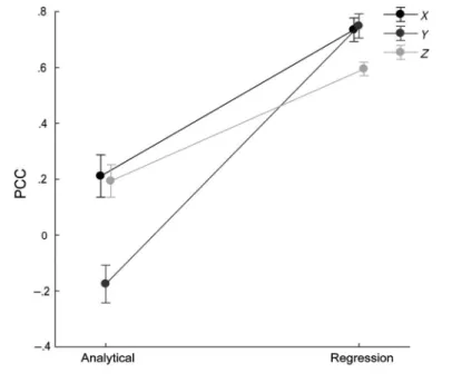
The MANOVA of the correlation between the estimated and measured ﬁngertip-position deviations from the mean revealed a signiﬁcant effect of method, F(3, 12) = 53.93, p< .001. The separate univariate analysis of variances on the X: F(1, 14) = 53.34, p< .001; Y: F(1, 14) = 112.57, p < .001; and Z directions: F(1, 14) = 47.18, p< .001, indicated that PCCs were higher in the regression method compared with the analytical method in all directions (see Figure1). Figure2, which depicts the relations betweenΔ^rjandΔrjfor a participant with low and a participant with high

ﬁngertip variability, elucidates that the linearized model created with the regression

Figure 1 — Means and SEs of the correlations between Δ^rjandΔrjfor the analytical and

the regression method to compute the linear model and each dimension of the position of the indexﬁnger (X, Y, and Z). PCC = Pearson correlation coefﬁcient.

(10)

method revealed a higher correlation between Δ^rj and Δrj in all movement

directions (PCCs> .42; see Figure 2, lower panels) than that of the analytical method (PCCs< .17; see Figure2, top panels) for participants with low and high ﬁngertip variability. To check whether the regression method had higher correla-tions than the analytical method for the complete movement, we also calculated the correlations betweenΔ^rjandΔrjat each instant of the (time-normalized) movement

trajectory. Visual inspection of these correlations also revealed higher correlations Figure 2 — Relations between Δ^rjof the linearized model andΔrjfor each method in a

separate plot and each direction in a different color (top row: analytical method; bottom row: regression method). The dashed black line represents the hypothesis whereΔ^rjandΔrjshow

a PCC of 1. The left panels show the least variable participant and the right panels the most variable participant (end-effector variability). The shades of gray for the different directions are as follows: X direction in dark gray, Y direction in gray, and Z direction in light gray. Note that the axes of the upper panels are different from the axes of the lower panels. PCC = Pearson correlation coefﬁcient.

(11)

for the linearized model created with the regression method than for the analytical method in 100% of the instances in all movement directions. Taken together, these results supported our expectation that the estimated position deviations from the mean of the index ﬁnger computed using the regression-based linear model described the data better than those computed using the analytical linear model.

Relation Between Fingertip Variability and NGEV

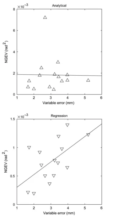
The PCC of the relation between theﬁngertip variability and NGEV (see Figure3) was medium to high in the linear model created with the regression method (r = .59), whereas it was very low in the model created using the analytical method (r =−.01). This result suggested that in the linear regression model joint-angle variability was partitioned into NGEV when appropriate, whereas this was not the case in the analytical model.

GEV and NGEV

The MANOVA of GEVlogand NGEVlogcomparing the models generated by the

two methods revealed a signiﬁcant method effect, F(2, 13) = 7.94, p = .006. Separate univariate analysis of variances on GEVlog and NGEVlog indicated

that, in the regression-based model, more joint-angle variability was partitioned into GEVlog, F(1, 14) = 14.02, p = .002, and less into NGEVlog, F(1, 14) = 16.67,

p = .001, than in the analytical-based model (see Figure 4). Given the small variability of the position of the index ﬁnger, these results suggested that the linear model created through regression described the data best.

To examine the orientations of the Jacobians for the two methods, we compared the null-space and orthogonal space of both Jacobians separately using the cosine of principle angles and found the averages across participants to be higher than the similarity criterion of 0.9 for theﬁrst four dimensions of the null-space and for all three dimensions of the orthogonal null-space. This indicated that the differences between the Jacobians of the regression and analytical methods used to create the linear model were in theﬁfth and the sixth dimensions of the null-space, implying that the subspaces of the two Jacobians were different, and, therefore, that the regression-based and analytical Jacobians were indeed different, and the differences between the two methods on the other measures were valid.

Discussion

When multijoint coordination is studied with the UCM method, the linear model is usually created using the analytical method rather than a regression method. One major difference between the two approaches is that in the analytical method only the averages of joint angles are used, whereas in the regression method the distribution of angular values of the joints and positional values of the end-effector across repetitions are used. Comparing the two linear models using data obtained in a manual reaching task, wefirst found higher correlations between the estimated and the measuredfingertip-position deviations from the mean in the regression-based linear model. Second, the relationship between fingertip variability and NGEV indicated that, if the linear model was created with the regression method,

(12)

Figure 3 — The relation between ﬁngertip variability and NGEV for each method, where each triangle represents one participant. Note that the y axis of the upper panel is different from the y axis of the lower panel. NGEV = nongoal-equivalent variability.

(13)

an appropriate amount of joint-angle variability was partitioned into NGEV, whereas this was not the case if the linear model was created analytically. Moreover, we showed that with the regression method more joint-angle variability was partitioned into GEV and less into NGEV. Taken together, these results demonstrated that the linear model created with the regression method provided a more accurate description of the data in the goal-directed reaching task, which is why we propose using the regression method to create the linear model for UCM analysis when analyzing reaching data.

Although we only examined goal-directed reaching, we argue that this recommendation can be extended to other actions, such as in sit-to-stance or walking. We hypothesized that the regression method described the data better than the analytical method because it incorporated the distribution of the joint angles and fingertip positions across repetitions into the linear model, whereas the analytical method considered only the averages of the joint angles and origins of the segments. Confirming our assumption, we have shown the added value of including these changes across repetitions in the analysis. Given that the distribu-tion of the data across repetidistribu-tions of the performance variable and the elemental variables also plays a role in other motor tasks, including this distribution in the creation of the model may also improve the linear model for these tasks. Note that this recommendation applies only to tasks in which the linear model has to be approximated. In tasks that are by definition linear, the regression method should not be considered. This is, for instance, the case in afinger force-production task where a certain amount of force needs to be exerted with fourfingers (DoF) at a Figure 4 — Means and SEs of the means of GEV and NGEV for the analytical and the regression method. NGEV = nongoal-equivalent variability; GEV = goal-equivalent variability; DoF = degrees of freedom.

(14)

certain point in time (Kang, Shinohara, Zatsiorsky, & Latash, 2004;Shinohara, Scholz, Zatsiorsky, & Latash, 2004). Here, the production of the total force is a linear combination of the four DoF and hence an exact linear model, which makes the use of the regression method superﬂuous. It is for tasks that require a linear approximation (i.e., tasks that are not exactly linear) that we suggest using the regression method to describe the data more accurately.

To do a UCM analysis of a reaching task, a linear approximation of the relations between changes in joint angles and changes infingertip position is used, although these relations are actually nonlinear (Latash et al., 2007; Schöner & Scholz, 2007). This is exemplified by a 3D plot with a curved (nonlinear) solution manifold in which three joint angles (three axes) keep thefingertip at one specific location at an instant in time. If the joint-angle ranges across repetitions are small, only a small part of this curved manifold is exploited, allowing this part to be approximated by a linear model because in a small part of the manifold the deviations from linearity are small. Given that in our simple reaching task the ranges of the joint-angle rotations across repetitions are small and the estimated deviations from the mean of thefingertip do not differ much from the measured deviations from the mean, the nonlinear behavior is suitable for approximation using a linear model (Ambike, Mattos, Zatsiorsky, & Latash, 2016;Jacquier-Bret, Rezzoug, & Gorce, 2009;Scholz & Schöner, 1999), facilitating the UCM analysis. While in the current task linearization is appropriate, in other tasks where the ranges of joint angles (or other elemental variables) across repetitions is larger, and thus also the scattering of trials on the curved solution manifold, a linearized manifold to approximate the solution manifold is less suitable. In such cases, one might consider using a nonlinear method to assess variability across trials. Müller and Sternad (2003), for example, proposed a surrogate nonlinear data analysis that was adapted and applied by Ambike et al. (2016; see alsoReschechtko & Latash, 2017) for an inverse pianofinger-force task. Having created a surrogate dataset by randomizing the original dataset, they found the surrogate dataset to show a much larger variance than the original one, implying that there was less covariance in the surrogate dataset and indicating that in the original data the variance was mainly covariance along the nonlinear solution manifold. In short, if the joint-angle ranges in a multijoint task are small, the usage of a linearized model is appropriate, whereas if the joint-angle ranges are larger a nonlinear method would be the better option. Note that there are also other discussions regarding the analysis of variability in redundant tasks (Sternad, 2018; Sternad, Park, Muller, & Hogan, 2010), but these are beyond the scope of this paper.

In conclusion, our results show that in goal-directed reaching the regression method to create the linear model is preferred to the analytical method. We argue that if UCM analysis is applied to tasks that require approximation of the linear model, the use of the regression method to create the linear model should be considered.

Acknowledgments

The project leading to this publication has received funding from Excellence Initiative of Aix-Marseille University—A*MIDEX, a French “Investissements d’Avenir” program. The authors have no conﬂict of interest related to the present study. They thank the ecological psychology journal club for the fruitful discussion about an earlier version of this paper.

(15)

They thank Tarkeshwar Singh, Hendrik Reimann, and Jorge Ibá˜nez-gijo´n for their helpful comments in response to an earlier version of the manuscript.

References

Ambike, S., Mattos, D., Zatsiorsky, V.M., & Latash, M.L. (2016). Synergies in the space of control variables within the equilibrium-point hypothesis. Neuroscience, 315, 150–161. PubMed ID:26701299doi:10.1016/j.neuroscience.2015.12.012

Black, D.P., Smith, B.A., Wu, J., & Ulrich, B.D. (2007). Uncontrolled manifold analysis of segmental angle variability during walking: Preadolescents with and without Down syndrome. Experimental Brain Research, 183, 511–521. PubMed ID: 17717659

doi:10.1007/s00221-007-1066-1

Cohen, J. (1988). Statistical power analysis for the behavioral sciences. Hillsdale, MI: Lawrence Erlbaum Associates.

de Freitas, S.M., & Scholz, J.P. (2010). A comparison of methods for identifying the Jacobian for uncontrolled manifold variance analysis. Journal of Biomechanics, 43(4), 775–777. PubMed ID:19922938doi:10.1016/j.jbiomech.2009.10.033

de Freitas, S.M., Scholz, J.P., & Latash, M.L. (2010). Analyses of joint variance related to voluntary whole-body movements performed in standing. Journal of Neuroscience Methods, 188(1), 89–96. doi:10.1016/j.jneumeth.2010.01.023

Domkin, D., Laczko, J., Djupsjöbacka, M., Jaric, S., & Latash, M.L. (2005). Joint angle variability in 3D bimanual pointing: Uncontrolled manifold analysis. Experimental Brain Research, 163, 44–57. PubMed ID:15668794doi:10.1007/s00221-004-2137-1

Golub, G.H., & Loan, C.F.V. (1996). Matrix computations. Baltimore, MD: Johns Hopkins University Press.

Greve, C., Zijlstra, W., Hortobágyi, T., & Bongers, R.M. (2013). Not all is lost: Old adults retain ﬂexibility in motor behavior during sit-to-stand. PLoS ONE, 8(10), e77760. PubMed ID:24204952doi:10.1371/journal.pone.0077760

Jacquier-Bret, J., Rezzoug, N., & Gorce, P. (2009). Adaptation of jointﬂexibility during a reach-to-grasp movement. Motor Control, 13(3), 342–361. PubMed ID:19799170

doi:10.1123/mcj.13.3.342

Kang, N., Shinohara, M., Zatsiorsky, V.M., & Latash, M.L. (2004). Learning multi-ﬁnger synergies: An uncontrolled manifold analysis. Experimental Brain Research, 157(3), 336–350. PubMed ID:15042264doi:10.1007/s00221-004-1850-0

Klous, M., Danna-dos-Santos, A., & Latash, M.L. (2010). Multi-muscle synergies in a dual postural task: Evidence for the principle of superposition. Experimental Brain Research, 202(2), 457–471. PubMed ID:20047089doi:10.1007/s00221-009-2153-2

Krishnamoorthy, V., Scholz, J.P., & Latash, M.L. (2007). The use ofﬂexible arm muscle synergies to perform an isometric stabilization task. Clinical Neurophysiology, 118(3), 525–537. PubMed ID:17204456doi:10.1016/j.clinph.2006.11.014

Krüger, M., Borbély, B., Eggert, T., & Straube, A. (2012). Synergistic control of joint angle variability: Inﬂuence of target shape. Human Movement Science, 31, 1071–1089.

doi:10.1016/j.humov.2011.12.002

Latash, M.L., Scholz, J.P., & Schöner, G. (2007). Toward a new theory of motor synergies. Motor Control, 11, 276–308. PubMed ID:17715460doi:10.1123/mcj.11.3.276

Maxwell, S.E., & Delaney, H.D. (1990). Designing experiments and analyzing data. Paciﬁc Grove, CA: Brooks/Cole Publishing Company.

Muceli, S., Falla, D., & Farina, D. (2014). Reorganization of muscle synergies during multidirectional reaching in the horizontal plane with experimental muscle pain. Journal of Neurophysiology, 111(8), 1615–1630. PubMed ID: 24453279 doi:10. 1152/jn.00147.2013

(16)

Müller, H., & Sternad, D. (2003). A randomization method for the calculation of covariation in multiple nonlinear relations: Illustrated with the example of goal-directed move-ments. Biological Cybernetics, 89, 22–33.

Reschechtko, S., Latash, M.L. (2017). Stability of hand force production. I. Hand level control variables and multiﬁnger synergies. Journal of Neurophysiology, 118(6), 3152–3164. PubMed ID:28904102doi:10.1152/jn.00485.2017

Romero, V., Kallen, R., Riley, M.A., & Richardson, M.J. (2015). Can discrete joint action be synergistic? Studying the stabilization of interpersonal hand coordination. Journal of Experimental Psychology: Human Perception and Performance, 41(5), 1223–1235. PubMed ID:26052696doi:10.1037/xhp0000083

Scholz, J.P., & Schöner, G. (1999). The uncontrolled manifold concept: Identifying control variables for a functional task. Experimental Brain Research, 126(3), 289–306. PubMed ID:10382616doi:10.1007/s002210050738

Scholz, J.P., Schöner, G., & Latash, M.L. (2000). Identifying the control structure of multijoint coordination during pistol shooting. Experimental Brain Research, 135, 382–404. PubMed ID:11146817doi:10.1007/s002210000540

Schöner, G., & Scholz, J.P. (2007). Analyzing variance in multi-degree-of-freedom move-ments: Uncovering structure versus extracting correlations. Motor Control, 11(3), 259–275. doi:10.1123/mcj.11.3.259

Shim, J.K., Hsu, J., Karol, S., & Hurley, B.F. (2008). Strength training increases training-speciﬁc multiﬁnger coordination in humans. Motor Control, 12, 311–329. PubMed ID:

18955741doi:10.1123/mcj.12.4.311

Shinohara, M., Scholz, J.P., Zatsiorsky, V.M., & Latash, M.L. (2004). Finger interaction during accurate multi-ﬁnger force production tasks in young and elderly persons. Experimental Brain Research, 156(3), 282–292. PubMed ID:14985892doi:10.1007/ s00221-003-1786-9

Sternad, D. (2018). It’s not (only) the mean that matters: Variability, noise and exploration in skill learning. Current Opinion in Behavioral Sciences, 20, 183–195. doi:10.1016/ j.cobeha.2018.01.004

Sternad, D., Park, S.W., Muller, H., & Hogan, N. (2010). Coordinate dependence of variability analysis. PLoS Computational Biology, 6(4), e1000751. PubMed ID:

20421930doi:10.1371/journal.pcbi.1000751

Togo, S., Kagawa, T., & Uno, Y. (2016). Changes in motor synergies for tracking movement and responses to perturbations depend on task-irrelevant dimension constraints. Human Movement Science, 46, 104–116. PubMed ID: 26741256 doi:10.1016/ j.humov.2015.12.010

Tseng, Y., Scholz, J.P., & Schöner, G. (2002). Goal-equivalent joint coordination in pointing: Affect of vision and arm dominance. Motor Control, 6(2), 183–207. PubMed

ID:12122226doi:10.1123/mcj.6.2.183

Valk, T.A., Mouton, L.J., & Bongers, R.M. (2016). Joint-angle coordination patterns ensure stabilization of a body-plus-tool system in point-to-point movements with a rod. Frontiers in Psychology, 7(826), 826.

van Andel, C.J., Wolterbeek, N., Doorenbosch, C.A.M., Veeger, D.H.E.J., & Harlaar, J. (2008). Complete 3D kinematics of upper extremity functional tasks. Gait & Posture, 27(1), 120–127. PubMed ID: 17459709 doi:10.1016/j.gaitpost.2007. 03.002

Van Der Steen, M.C., & Bongers, R.M. (2011). Joint angle variability and co-variation in a reaching with a rod task. Experimental Brain Research, 208, 411–422. PubMed ID:

21127846doi:10.1007/s00221-010-2493-y

Verrel, J. (2010). Distributional properties and variance-stabilizing transformations for measures of uncontrolled manifold effects. Journal of Neuroscience Methods, 191(2), 166–170. PubMed ID:20599556doi:10.1016/j.jneumeth.2010.06.016

(17)

Wu, G., Van Der Helm, F.C.T., Veeger, H.E.J., Makhsous, M., Van Roy, P., Anglin, C.,: : : Buchholz, B. (2005). ISB recommendation on deﬁnitions of joint coordinate systems of various joints for the reporting of human joint motion—Part II: Shoulder, elbow, wrist and hand. Journal of Biomechanics, 38(5), 981–992. PubMed ID:15844264doi:10. 1016/j.jbiomech.2004.05.042

Wu, Y.H., Pazin, N., Zatsiorsky, V.M., & Latash, M.L. (2012). Practicing elements versus practicing coordination: Changes in the structure of variance. Journal of Motor Behavior, 44(6), 471–478. PubMed ID: 23237469 doi:10.1080/00222895.2012. 740101

Yang, J.F., Scholz, J.P., & Latash, M.L. (2007). The role of kinematic redundancy in adaptation of reaching. Experimental Brain Research, 176, 54–69. PubMed ID:

16874517doi:10.1007/s00221-006-0602-8

Zaiontz, C. (2018). Real statistics using excel. Retrieved fromwww.real-statistics.com