A Computer oriented adaption of Salzer's method for inverting LaPlace transforms

(1)

Publisher’s version / Version de l'éditeur:

Journal of Mathematics and Physics, 40, 2, pp. 135-141, 1961-10-01

READ THESE TERMS AND CONDITIONS CAREFULLY BEFORE USING THIS WEBSITE. https://nrc-publications.canada.ca/eng/copyright

Vous avez des questions? Nous pouvons vous aider. Pour communiquer directement avec un auteur, consultez la

première page de la revue dans laquelle son article a été publié afin de trouver ses coordonnées. Si vous n’arrivez pas à les repérer, communiquez avec nous à PublicationsArchive-ArchivesPublications@nrc-cnrc.gc.ca.

Questions? Contact the NRC Publications Archive team at

PublicationsArchive-ArchivesPublications@nrc-cnrc.gc.ca. If you wish to email the authors directly, please see the first page of the publication for their contact information.

NRC Publications Archive

Archives des publications du CNRC

This publication could be one of several versions: author’s original, accepted manuscript or the publisher’s version. / La version de cette publication peut être l’une des suivantes : la version prépublication de l’auteur, la version acceptée du manuscrit ou la version de l’éditeur.

Access and use of this website and the material on it are subject to the Terms and Conditions set forth at

A Computer oriented adaption of Salzer's method for inverting LaPlace

transforms

Shirtliffe, C. J.; Stephenson, D. G.

https://publications-cnrc.canada.ca/fra/droits

L’accès à ce site Web et l’utilisation de son contenu sont assujettis aux conditions présentées dans le site LISEZ CES CONDITIONS ATTENTIVEMENT AVANT D’UTILISER CE SITE WEB.

NRC Publications Record / Notice d'Archives des publications de CNRC:

https://nrc-publications.canada.ca/eng/view/object/?id=5f7f28d7-2ae2-4ea3-a02b-16b23be77223 https://publications-cnrc.canada.ca/fra/voir/objet/?id=5f7f28d7-2ae2-4ea3-a02b-16b23be77223

(2)

Ser TH1

N21r2

no.

140

c . 2

NATIONAL

RESEARCH

COUNCIL

C A N A D A

DIVISION OF BUILDING RESEARCH

A COMPUTER ORIENTED ADAPTION OF SALZER'S METHOD

FOR INVERTING LAPLACE TRANSFORMS

BY

C. J. SHlRTLlFFE AND D. G. STEPHENSON

REPRINTED F R O M

J O U R N A L OF M A T H E M A T I C S A N D P H Y S I C S , V O L . XL, N O . 2. J U L Y 1961, P. 135

-

141.

RESEARCH PAPER N O . 140

O F T H E

DIVISION OF BUILDING RESEARCH

OTTAWA OCTOBER 1961

(3)

T h i s p u b l i c a t i o n i s being d i s t r i b u t e d by t h e D i v i s i o n of Building R e s e a r c h of t h e National R e s e a r c h Council. I t should not b e r e p r o d u c e d i n w h o l e o r i n p a r t , without p e r m i s - s i o n of t h e o r i g i n a l p u b l i s h e r . T h e D i v i s i o n would be glad to b e of a s s i s t a n c e i n obtaining s u c h p e r m i s s i o n .

P u b l i c a t i o n s of t h e Division of Building R e s e a r c h m a y b e obtained by m a i l i n g the a p p r o p r i a t e r e m i t t a n c e , ( a Bank, E x p r e s s , o r P o s t Office M a n e y O r d e r o r a cheque m a d e pay- a b l e a t p a r i n Ottawa, to t h e R e c e i v e r G e n e r a l of Canada, c r e d i t National R e s e a r c h Council) t o the National R e s e a r c h Council, Ottawa. S t a m p s a r e not a c c e p t a b l e .

A coupon s y s t e m h a s been i n t r o d u c e d to m a k e pay- m e n t s f o r p u b l i c a t i o n s r e l a t i v e l y s i m p l e . Caupons a r e a v a i l - a b l e i n d e n o m i n a t i o n s of 5, 2 5 and 50 c e n t s , and m a y b e ob- t a i n e d by m a k i n g a r e m i t t a n c e a s i n d i c a t e d above. T h e s e coupons m a y b e u s e d f o r t h e p u r c h a s e of a l l National R e s e a r c h Council p u b l i c a t i o n s including s p e c i f i c a t i o n s of t h e Canadian G o v e r n m e n t S p e c i f i c a t i o n s B o a r d .

(4)

Repririted i~.oln Joun~Ar, OF & f h ~ l r ~ h r h ~ r c s AND PAYBICJ Vol. XL, No. 2, July, 1961

1'~irrled in U . S . A .

A COMPUTER ORIENTED ADAPTION O F SALZER'S METHOD F O R I N V E n T I N G LAPLACE TRANSFORMS

Description of problem. Salzer's method [I] for nuinerically inverting a Laplace transform consists of fitting a Lagrange polynomial iir l / p to the trans- forin of the function and inverting the polynomial term by term. The polynomial is fitted to the values of the transform a t equal intervals along the positive real axis of the complex plane.

The calculation consists of summing a series of products of interpolation coefficients ancl values of the transform. It is only necessary to evaluate the transform with p equal to 1, 2, 3,

-

. .

m ; where nz is one less t,han the order of thc Lagraiige polynomial used.

The difficulty with this approach is that it is not possible to represent ac- curately every furiction by a polynomial which has poles only a t the origin. Such a polyilonlial iiivcrts to a power series which always approaches infinity as t,lle iildependeilt variable approaches infinity. Salzer's paper contaiils an expression ~vllich will give an estimate of the error in the numerical inverse, but it requires the conlputist to make an estimate of the mttL derivativc of F ( p ) with respect t o l / p . The method which follows avoids the need for this estinlate of a derivative and also indicates the optimum order of Lagrange polyilomial to use. T h e existence of an optimunl m was not mentioned by Salzer.

Salzer's expression for the inverse trallsform is

lj7)l+l

i I y ( t ) = --

C

a.j t"'-' m ! (7n - j ) !

a i d a, is one of a set of collstant coefficients of the nz

+

1 point Lagmmlgc inter- polatioil polynomial coefficients. It is a function of k ailcl is a n exact integer [2]. The values of i l r ( t ) arc tabulated i11 Salzer's paper for specific values of t.

A proglBam has beell prepared to allow a digital computer to evaluate the inverse tmnsform for ally value of t, using up to an 11-point Lagrange polynomial. The inversion is done using the follo~ving double series.

~vherc bi are a special set of constants derived from uj by

The values of bi for m = 2 t o 10 are given in Table I. The Bcndix computer users program [3] has these constants incorporated with the program on puilched paper tape. The values of b i have been checked against Salzer's tables by

(5)

T A B Tables of b i Interpolation Constants for N u n z e ~

NOTE. Tlie numbc1.s in t h c tuble 11re in a floating point form; t h e n u ~ n b c r a t the right is the cl~uracteristic. T l ~ e fo~rucrt is of places t o move the decinlrll to the left.

(6)

LE I

ical Calculalion o j Inverse Laplace Transjorms

f _{.DDDDDDDDDDDD} _{X S}_{\ v h r ~ c}_{X X is the number}of places to move the deci~nul to the right and, . . X X is the number

(7)

138 C. J. SRIRTLIFFE AND D. G. STEPHENSON

The values of AT(1) thus calculated have more sigllificant figures t h a n are given in Salzer's paper hut when they are rounded t o the same number of digits the agreement is perfect.

The values o f f ( t ) determined using different values of m should be the same (independent of m ) so long as they are correct. Thus a comparison of the results of a series of calculations with successive values of m indicates the illaximum value of t for which the value of f ( t ) is accurate. The results also show t h e optimum value of m.

The computer has been used to invert the following transforms for several values of the pole positions:

These trailsforms werc studied because of the position of tlicir poles and because the exact values of the inverse transforms wcl-e readily available.

Results. It was found t h a t increasing the order of the Lagrange polynomial (i.e. the value of ~ n ) did not necessarily increase the rangc or accuracy of the

m

1 Fro. 1. Precision of numericnl irivelvion of

(8)

INVERTING LAPLACE TRANSFORMS

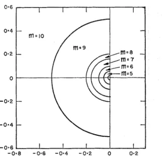
FIG. 2. Dependence of optimmn on position of poles i n p-plane

inverse transform. For each function there is an optimum nz which will give the least error in f ( t ) over the greatest range of t. For exact polynomials in l / p t h e optinlum m obviously corresponds to the highest power of l l p . When F ( p ) is not a11 exact polyilonlial in l / p the optimum value of m seems to depend pri- marily on the position of the poles of F ( p ) .

Figure 1 shows a typical variation in error with m and t for poles at f i ( O . 1 ) . 13y making similar evaluatio~ls for the inversio~ls of l / ( p

+

b ) , l / ( p 2

+

b 2 ) , a n d

l / [ ( p

+

c)" dd?] it was possible to establish an approxinlate relationship be- tween the pole position and the optimum nz. This is shown graphically in Fig. 2. This relationship is of no practical value in finding the optimum m since the poles of F ( p ) are not usually kno~~~vvn.

The optinlum 7n and the upper limit of t can both be found by repeated appli-

cation of the numerical inversion using successive values of m. I n this way t h e results which agree to the highest t for three consecutive values of m can be found. The optimum value is the middle one of the three. Figure 3 sho\vs the values of f ( t ) calculated using values of m from 4 to 9, for F ( p ) = l / ( p 2

+

( 0 . 1 ) ' ) . The optimum m is seen to be seven. The error in the inversion obtained wit11 the optimum m is less than half the difference between i t and the values obtaiiled when m is one larger and one smaller than the optimum. Therefore, once the optinlum m has been found the limits on the error are indicated without any further calculation.

The method for finding the opt,imum m only works when the optimum is less than 10 since only the 3 to 11 point interpolation fornlulas are used. It is possible to distinguish cases where the optimum m is 10 or only slightly greater from cases where it is much greater than 10 by examining the difference in the values of the inversion a t t = 0 for m = 9 and m = 10. If the difference is large, t h e

(9)

C. J. SHIRTLIFFE AND D. G. STEPI-IENSON I I I I I I 10.0

-

9 . 0

-

8 . 0

-

+

7.0

-

5.0

-

4 V Y- LEGEND: 0 CORRECT b 2.0

-

.

_{m = 4}

-

A m = 5 A m = 6

-

0 _{m = 7} a m = s + m = 9

-

1 1 1 1 1 1 1 1 1 1 l 1 1 1 1 0 0.4 0 . 8 1.2 1.6 2 . 0 2 . 4 2.8 3.

b t

optimum m is considerably greater than 10 and the method caililnot be used. If the difference is less than the allowable error, the optimum m is 10 or near enough to 10 that the method can be used. The limit on the error caililot be found by the usual method in such cases. If the values for a particular t a t nz = 9

and m = 10 agree within the allowable error, however, the error in the inversion using m = 10 will not exceed the allowable error.

It would be possible t o calculate the Lagrange iilterpolation constants for m's higher than 10. The greater the m, however, the greater the number of significant figures lost in the summation. The number lost can exceed 12 using m = 10 and t = 10. The maximum usable m would therefore depend on the computer used for the calculations. The transform must be defined t o more figures than the number of significant figures dropped in the calculation, hom- ever, there is no advantage in having the transform defined to more figures tlian the constants.

(10)

INVERTING LAPLACE TRANSFOR~VS 141

Acknowledgment. This paper is a contribution froin the Division of Building Research of the National Research Council of Canada and is published with the approval of the Director of the Division.

REFERENCES

1. SALZER, El. E . , Tables for the Nulnerical Calculation of Inverse Laplace Transforms. J. Math. and Phys., 37, 1958, p. 89-108.

2. SALZER, H. E., Tables of Coefficients for the Numerical Calculation of Laplace Trans- forms. National Bureau of Standards, Applied Mathematics Series No. 30 U. S. Government Printing Office, Washington, D . C., 1953, 3G p.

3. SIII~ZTLIFFE, C. J., Nun~erical Calculation of Inverse Laplace Transforms. Bendix Users Project. Library Program U 538.