A Psychophysical Evaluation of Texture Compression Masking Effects

HAL Id: hal-01719531

https://hal.archives-ouvertes.fr/hal-01719531

Submitted on 28 Feb 2018

HAL is a multi-disciplinary open access

archive for the deposit and dissemination of

sci-entific research documents, whether they are

pub-lished or not. The documents may come from

teaching and research institutions in France or

abroad, or from public or private research centers.

L’archive ouverte pluridisciplinaire HAL, est

destinée au dépôt et à la diffusion de documents

scientifiques de niveau recherche, publiés ou non,

émanant des établissements d’enseignement et de

recherche français ou étrangers, des laboratoires

publics ou privés.

Masking Effects

Guillaume Lavoué, Michael Langer, Adrien Peytavie, Pierre Poulin

To cite this version:

Guillaume Lavoué, Michael Langer, Adrien Peytavie, Pierre Poulin.

A Psychophysical

Evalua-tion of Texture Compression Masking Effects.

IEEE Transactions on Visualization and

Com-puter Graphics, Institute of Electrical and Electronics Engineers, 2019, 25 (2), pp.1336 - 1346.

�10.1109/TVCG.2018.2805355�. �hal-01719531�

A Psychophysical Evaluation of Texture

Compression Masking Effects

Guillaume Lavou ´e, Senior Member, IEEE, Michael Langer, Adrien Peytavie and Pierre Poulin.

Abstract—Lossy texture compression is increasingly used to reduce GPU memory and bandwidth consumption. However, as raised by recent studies, evaluating the quality of compressed textures is a difficult problem. Indeed using Peak Signal-to-Noise Ratio (PSNR) on texture images, like done in most applications, may not be a correct way to proceed. In particular, there is evidence that masking effects apply when the texture image is mapped on a surface and combined with other textures (e.g., affecting geometry or normal). These masking effects have to be taken into account when compressing a set of texture maps, in order to have a real understanding of the visual impact of the compression artifacts on the rendered images. In this work, we present the first psychophysical experiment investigating the perceptual impact of texture compression on rendered images. We explore the influence of compression bit rate, light direction, and diffuse and normal map content on the visual impact of artifacts. The collected data reveal huge masking effects from normal map to diffuse map artifacts and vice versa, and reveal the weakness of PSNR applied on individual textures for evaluating compression quality. The results allow us to also analyze the performance and failures of image quality metrics for predicting the visibility of these artifacts. We finally provide some recommendations for evaluating the quality of texture compression and show a practical application to approximating the distortion measured on a rendered 3D shape.

Index Terms—Texture compression, psychophysical experiment, image quality assessment, diffuse map, normal map.

F

1

I

NTRODUCTION

T

HREE dimensional graphical objects are now commonplace in many fields of industry, including digital entertainment, computational engineering, and cultural heritage. They commonly consist of geometric surfaces on which one or more textures are mapped to make their rendering more realistic. Multiple texture maps are usually considered (e.g., affecting surface geometry or normal, or reflectance terms such as diffuse, gloss, specular) to reproduce accurately physical characteristics of surface materials (e.g., albedo, microsurface, reflectivity), and thus to generate highly realistic scenes.

These textures are mostly stored in some form of images and, in most cases, subjected to lossy compression. This compression may occur either to fasten streaming and remote visualization of the 3D scene (in that case, variable-bit-rate methods may be used such as JPEG or JPEG2000 [1]) or to reduce storage on the graphics processing unit (GPU) (using GPU-friendly random-access methods such as [2], [3], [4]). As raised by Olano et al. [5], texture compression will always be necessary in interactive applications such as games, since it allows for more texture data to reside on the GPU. That way, compression decreases data transfers to GPU, and it thus reduces latency and/or allows for more detailed textures to be used. Lossy compression introduces artifacts that may impact the visual quality of the rendered 3D scene. Consequently, compression has to be carefully driven and evaluated by accurate metrics. The most common approach in evaluating texture compression is to

• G. Lavou´e and A. Peytavie are with the CNRS, Univ. Lyon, LIRIS, France E-mail: glavoue@liris.cnrs.fr.

• M. Langer is with the McGill University, Canada.

• P. Poulin is with the Universit´e de Montr´eal, Canada.

use simple metrics (e.g., PSNR) or visual image inspection on individual textures. However, as raised by Griffin and Olano [6], inspecting individual textures is incorrect for two reasons: (1) Texture images are not visualized directly but are mapped onto 3D shapes that are then shaded and rendered according to certain viewpoints and lighting configurations. Therefore, the perception of compression artifacts on a texture image may be very different than their perception on a rendered 3D scene (i.e., after shading, viewpoint selection, and rasterization). (2) One particular shape may often be rendered using several texture maps (e.g., diffuse and normal), even of different resolutions, that interact during rendering and may thus mutually mask their artifacts.

Griffin and Olano [6] have studied the two effects mentioned above (they refer to (1) as geometric masking and to (2) as texture-set masking). Their results tend to show that they significantly mask compression artifacts and that compression algorithms may be too conservative. However, these results are not based on a psychophysical quality study, but on outcomes from objective metrics (CIELAB δE94 and SSIM [7]) taken as perceptual oracles of perceived visual quality. As shown by recent studies [8], [9], [10], such image quality metrics may be very poor at evaluating artifacts on rendered 3D surfaces.

The goal of this work is similar to the one of Griffin and Olano [6], i.e., investigating the effect of geometric and texture-set masking on the perception of texture compression artifacts. However, in addition to using objective metrics, we conducted two psychophysical experiments (Sec. 3). Our statistical analysis (Sec. 4) quantitatively demonstrates the impact of these masking effects on artifact detection thresholds, as well as the influence of light direction and texture content. We also used the psychophysical data

to evaluate the performance of image quality metrics for predicting the visibility of these artifacts (Sec. 5) and make some recommendations for optimizing the quality of texture compression (Sec. 6). We finally demonstrate the practical use of theses recommendations in a realistic application (Sec. 7).

2

R

ELATED WORK

We are interested in evaluating the quality of rendered scenes, subjected to compression of their texture maps applied on surfaces. We review here, briefly, the existing work in visual quality assessment for 3D scenes; for a more complete recent survey of this field we refer the reader to [11].

Near-threshold Image Metrics. For 2D natural images, research into objective quality assessment metrics is substantially developed [12]. Bottom-up techniques try to mimic the low-level mechanisms of the human visual system (HVS) such as the contrast sensitivity function (CSF), usually modeled by a band-pass filter, and the visual masking effects that define the fact that one visual pattern can hide the visibility of another. They include the Sarnoff Visual Discrimination Model (VDM) [13], the Visible Difference Predictor (VDP) [14], and the more recent HDR-VDP-2 [15], suited for any range of luminance. These bottom-up approaches usually focus on near-threshold visual models and produce maps of just-noticeable differences. They have been extensively used in computer graphics for perceptually-based rendering, e.g., to reduce and/or optimize the number of samples of global illumination algorithms [16], [17], [18], and for simplification and Level of Detail (LoD) selection [19], [20], [21], [22].

Supra-threshold Image Metrics. The near-threshold models described above are usually not suited to characterize supra-threshold perceptual distortions. In contrast, some authors propose top-down metrics that do not take into account any HVS model, but instead that operate based on some intuitive hypotheses of what HVS attempts to achieve when shown a distorted image. The most well-known example is the Structural SIMilarity index (SSIM) [7]. A large number of top-down image quality metrics have been proposed since then [23], [24], [25], the most recent being data-driven, i.e., the metrics are learned based on user studies [26], [27], [28]. Several authors use these top-down metrics for visual quality evaluation in computer graphics. Zhu et al. [29] study the relationship between viewing distance and perceptibility of model details using SSIM [7], while Griffin and Olano [6] use this metric to evaluate the visual impact of texture map compression. SSIM is also used by Brady et al. [30] and Havran et al. [31] to evaluate quality of Bidirectional Reflectance Distribution Functions (BRDFs), using rendered images.

Metrics Dedicated to Rendering Artifacts. Most of the quality metrics presented above have been designed and evaluated on natural images with mostly compression/transmission related artifacts (e.g., Gaussian noise, JPEG artifacts). A recent study [8] has shown that

they are not suited for evaluating artifacts introduced by rendering in synthetic images, e.g., aliasing or noise from global illumination approximations. Several authors have recently introduced quality metrics specifically dedicated to this kind of rendering artifacts [32], [33], [34].

Metrics for 3D Mesh. While the metrics above operate in image space, several authors have proposed metrics that operate directly in the space of 3D meshes. They mostly rely on geometry characteristics, such as curvature [35], dihedral angles [36], or roughness [37]. Some of them combine geometry difference with a difference in diffuse texture maps [10], [38].

Metrics for BTF. Filip et al. [39] and Guthe et al. [40] introduce quality metrics for Bidirectional Texture Functions (BTFs), with the goal of driving their compression. Jarabo et al. [41] evaluate the impact of approximate filtering on the appearance of BTFs, with respect to their characteristics (e.g., structure, roughness, contrast). While the purpose of this latter study is different from ours, it has been inspiring to us since we also want to evaluate the impact of different characteristics (texture content, compression strength, lighting) on the detection of artifacts.

The objective of our experiment is to study the impact on rendered images of artifacts coming from texture com-pression (diffuse and normal). Collected data will allow us to assess if image quality metrics presented above are able to correctly evaluate the perceptual impact of such artifacts.

3

P

SYCHOPHYSICAL EXPERIMENTS

We conduct two psychophysical studies to explore masking effects caused by the normal map on the perception of the diffuse map compression artifacts and vice versa. Here we describe the dataset and protocol in more details.

3.1 Stimuli

3.1.1 Texture Maps

We selected four pairs of diffuse/normal texture maps and a flat stimulus, all illustrated in Figure 1. They represent typical materials used by designers and exhibit a variety of characteristics, and thus of potential masking effects. The diffuse maps come from photographs of real surfaces, and normal maps have been created from the diffuse maps (a standard process in texture design). Their characteristics are detailed in Table 1 in the form of high-level properties inspired from previous work on texture [42] and BTF [41] classifications.

TABLE 1

Characteristics of our five texture pairs.

Texture Normal

content amplitudes

Flat Uniform Zero

Stones Random (non-uniform), sharp sparse edges Low Water Random (non-uniform), Low Frequency Low

Hedge Random (uniform), Medium frequency High

Dif

fuse

Normal

Flat Stones Water Hedge Fabric Fig. 1. Our five reference diffuse (top) and normal (bottom) texture maps.

Following Griffin and Olano [6], we have considered texture maps corresponding to a traditional real-time shad-ing workflow, as opposed to a Physically-based Rendershad-ing (PBR) workflow. In traditional real-time shading, the diffuse texture maps contain not only the albedo but also contain pre-rendered photometric effects to ensure the rendered surface has visible features whatever lighting conditions. Examples are global illumination effects such as ambient occlusion which occur in Hedge, and specular reflections and refraction which occur in Water.

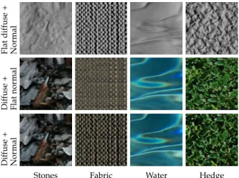
Figure 2 illustrates the rendering of our texture pairs (indi-vidual and combined together), mapped on a plane and lit using directional lighting. As can be observed in this figure, diffuse and normal maps are strongly correlated. However, this does not impact the generality of our study since in our psychophysical experiments every diffuse map is combined with every normal map.

Flat dif fuse + Normal Dif fuse + Flat normal Dif fuse + Normal

Stones Fabric Water Hedge

Fig. 2. Rendered texture maps (normal only, diffuse only, and both), on a textured Lambertian 3D square lit from the left.

We specifically selected small texture patches (128 × 128) to restrict where the user is looking, and to prevent long spatial exploration that could potentially occur with larger stimuli.

3.1.2 Compression

These texture maps have then been compressed by the ASTC algorithm [3]. ASTC is a lossy block-based compres-sion algorithm that represents the state of the art in terms of performance. It encodes each block using 128 bits; hence, by adjusting the size (in texture pixels, i.e. texels) of the blocks, it can produce a large variety of output qualities. The

larger the block size is, the more efficient is the compression, and the larger (and more visible) are the block artifacts. For each reference texture map, we created 5 lossy compressed versions corresponding to 5 block sizes: 6 × 6, 8 × 8, 10 × 10, 12×10, and 12×12, that correspond respectively to bit rates: 3.56, 2.00, 1.28, 1.07, and 0.89 bits per pixel. These sizes have been adjusted during a pilot experiment in order to enclose the detection thresholds for all our reference diffuse and normal maps. We used the ARM Mali GPU Texture Com-pression Tool [43] with comCom-pression mode set to fast. Nor-mal maps were compressed using the norNor-mal psnr mode. Examples of compression artifacts are illustrated in Figure 3. One can observe that block artifacts highly depend on the maps. For instance, 8 × 8 artifacts are clearly identifiable in the Water diffuse map but much more difficult to perceive in the Fabric one.

Dif

fuse

Normal

Water6×6 Water8×8 Water12×12 Fabric8×8 Fabric12×12

Fig. 3. Examples of compressed diffuse (top) and normal (bottom) texture maps, for different block sizes of the ASTC algorithm [3].

3.1.3 Rendering

Normal Masking Experiment

The first experiment studies the masking effects caused by the normal map on the perception of the diffuse map compression artifacts. For each compressed diffuse texture image, except for Flat (4 maps × 5 compression levels = 20 images), we make one rendering with every normal map (5 maps) and using 2 light directions; we thus rendered 200 images.

For rendering, the diffuse and normal images are mapped onto a geometric 3D square of Lambertian reflectance. We set a directional light from the left with two directions: 0◦ and 42.5◦ from the normal direction of the square. The scenes are rendered by ray-tracing using the Mental Ray software [44]. Figure 4 illustrates some rendered results. The rendered images of resolution 128 × 128 respect the usual setting of one pixel per texel for ideal rendering.

Fabric,Hedge,42 Water,Fabric,0 Water,Fabric,42 Stones,Fabric,0 Hedge,Water,42 Fig. 4. Examples of stimuli for the Normal Masking experiment. Triplets indicate: diffuse map, normal map, light direction. Light comes from the left. Diffuse maps are compressed with block size10 × 10.

Diffuse Masking Experiment

The second experiment studies the masking effects caused by the diffuse texture maps on the perception of the normal

maps compression artifacts. For this experiment we remove the Stones stimulus since its normal map is of low ampli-tude and compression artifacts remain invisible whatever our compression parameters. Consequently, we select the 3 remaining normal maps × 5 compression levels, and render with 4 diffuse maps (Flat, Fabric, Water, and Hedge) using 2 light directions; we thus render 120 images. To emphasize the visual impact of normals, we select 2 light directions: 27◦ and 72◦ from the viewing direction, also coming from the left. We do not select the 0◦direction since the effects of normals on the surface would be too small for human sub-jects to perceive artifacts. Figure 5 illustrates some rendered results. Note that images are not normalized, i.e., scenes lit from 72◦s are darker.

Flat,Water,27 Flat,Water,72 Water,Water,27 Fabric,Water,27 Fabric,Water,72 Fig. 5. Examples of stimuli for the Diffuse Masking experiment. Triplets indicate: diffuse map, normal map, light direction. Light comes from the left. Normal maps are compressed with block size12 × 12.

3.2 Procedure

Our two psychophysical experiments aim to measure thresholds for detecting artifacts. They follow the same ran-domized two-alternative-choice (2AFC) design. Each sub-ject is shown triplets of rendered images, corresponding to the same diffuse/normal map combination. Images are displayed on a 50% grey background and the order of triplets is randomized. The reference rendering (without any compression) is displayed in the center. On left and right, two test images are displayed. One is the same as the reference and the other involves a compressed map (either diffuse or normal, depending on the experiment); their position (left or right) is randomized. Subjects were asked: ”Which image is different from the reference?” and clicked on the corresponding image. They were given a maximum of 8 seconds; after this time, a pop-up window asked them to choose. As in [39], this time limit aims to prevent subjects from making an exhaustive pixel-wise comparison of the images.

All stimuli were presented on a calibrated 17.3” LCD display (1920 × 1080 pixel resolution) in a dark room. A chin-rest was used to keep constant viewing distance of 0.35m, corresponding to an angular resolution of 33.5 pixels per degree. With our setting, each image subtends approxi-mately 3.8◦of visual angle. 22 paid subjects participated in the experiments. All were students from McGill university, aged between 18 and 33, with normal or corrected-to-normal vision. Each subject completed the two experiments. 11 did the Normal Masking one followed by the Diffuse Masking one, and 11 did the inverse. They took on average 35 minutes in total to perform both experiments.

4

D

ATA

A

NALYSIS

In this section we study the effect of light direction and texture content on the compression error detection threshold. We investigate, in particular, the involved masking effects.

4.1 Normal Masking Experiment

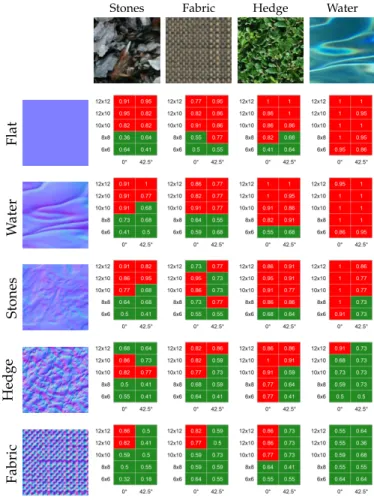
In this experiment, the normal texture potentially masks the compressed diffuse texture. Figure 6 illustrates the raw re-sults of this first experiment. The detection probabilities are displayed for each set of conditions. Green indicates visual equivalence to the reference (75% 2AFC threshold), while red means a visual difference. Figure 7 summarizes these results using boxplots of detection probabilities. Table 2 provides results of pairwise t-tests between each condition. We chose to represent these tables as n × (n − 1) matrices (for comparing n conditions), instead of n × n symmetric matrices with empty main diagonals. Each cell considers, for the two conditions, the distributions of detection proba-bilities. The following paragraphs discuss the effects of each parameter. Note that when the Flat normal is used (first row of Figure 6), what we are examining is not masking, but rather whether the compressed textures are distinguishable from original ones.

Stones Fabric Hedge Water

Flat W ater Stones Hedge Fabric

Fig. 6. Results of the Normal Masking experiment. Detection probabil-ities P are given for each pair of diffuse/normal maps, and for each compression level and light direction. Green means that rendered im-ages are considered identical (P < 0.75), while red means that visible differences are detected (P ≥ 0.75).

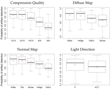
Compression Quality. The compression quality obviously influences the perceived visibility of artifacts. Larger block

Compression Quality Diffuse Map

Normal Map Light Direction

Fig. 7. Boxplots of detection probabilities obtained for the different con-ditions of each parameter, for the Normal Masking experiment (diffuse maps are compressed). Mean values are displayed as red circles.

TABLE 2

P-values from pairwise paired t-test (Bonferroni-corrected) between all conditions, for the Normal Masking experiment.

Compression Quality Diffuse Map

12×12 12×10 10×10 8×8 12×10 1.000 - - -10×10 0.122 1.000 - -8×8<0.001<0.001<0.001 -6×6<0.001<0.001<0.001<0.001

Water Hedge Fabric Hedge 1.000 -

-Fabric<0.001<0.001 -Stones<0.001<0.001 0.280

Normal Map Light Direction

Water Flat Stones Hedge Flat 1.000 - - -Stones 0.303 1.000 - -Hedge 0.001 0.002 0.011 -Fabric<0.001<0.001<0.001 0.003 42.5◦ 0◦_<0.001

sizes induce block artifacts that are both larger in size and in amplitude. Still, it is interesting to observe that there are no significant differences in detection probabilities between 10 × 10, 12 × 10, and 12 × 12 (see Table 2).

Diffuse Map.The content of the diffuse map influences the detection probabilities. Hedge and Water diffuse maps seem to be the most sensitive to compression, as illustrated by the large number of red cells in the last two columns of Figure 6, as well as their boxplots from Figure 7 (top right). Reasons are different: Hedge has many high-contrast sharp edges that are easily damaged by block artifacts, while Water is quite smooth with very low intrinsic masking effects.

Normal Map.When looking at Figures 6 and 7 (bottom left) it appears obvious that the normal map strongly influences the perception of diffuse map artifacts. For example, in Figure 6, for the Water diffuse map, visible differences are perceived for all compression ratios when combined with the Flat normal map, while no difference is perceived when combined with Fabric. The two critical factors that deter-mine masking effects are frequency and amplitude. In Fig-ure 7, Hedge and Fabric normal maps, which have highest

frequency and amplitude, lead to significantly lower detec-tion probabilities (see also Table 2, bottom left). A closer look reveals that for a given high amplitude (Hedge and Fabric), masking effects increase with frequency. Indeed, Fabric is of higher frequency and Fabrics masking effects are clearly stronger. Similarly, for a given low amplitude (Water and Stones), a high frequency and noisy texture provides slightly higher masking effects. However, low amplitude normal maps (Water and Stones) are not significantly different from the Flat one and lead to high detection probabilities. When carefully looking at Figure 6, the normal masking effects are slightly more complex. Indeed, all artifacts on the Water diffuse map are almost completely masked by Hedge and Fabric normal maps. However, the masking effects of these two normal maps are much lower for the other diffuse maps (i.e., Stones, Fabric, and Hedge). The masking effects brought by a normal map actually depend on the diffuse map content. Note that a strong correlation between diffuse and normal maps (as we have when we combine a diffuse/normal pair) does not seem to lower or increase the masking effects.

Light Direction.A significant impact due to light direction is observed. First, when the angle between light direction and surface normal increases, then the rendered image is darker, thus decreasing the contrast of the signal. Second, this masking is reinforced by the fact that non-perpendicular lighting emphasizes the influence of the normal map (which thus increases contrast-masking effects).

4.2 Diffuse Masking Experiment

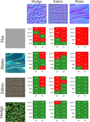
In this experiment, the diffuse map potentially masks the compressed normal map. As above, Figure 8 illustrates raw results, Figure 9 summarizes these results using boxplots of detection probabilities, and Table 3 provides results of pairwise t-tests between each condition. The following paragraphs discuss the effects of each parameter.

Compression Quality.We observe that when compressing normal maps, the level of compression has less impact on the perception of artifacts than when compressing diffuse maps. The visibility of artifacts actually mostly depends on the diffuse masking, as detailed below.

Normal Map. When looking at Figure 9 (top right) one could state that the content of the normal map itself does not seem to have a significant influence on the perception of artifacts. This is confirmed by Table 3 (top right). However, Figure 8 clearly shows that the normal map does have an influence, that is very strongly related to the masker. Indeed, as illustrated in the first two rows of Figure 8, with a weak masking (Flat or Water diffuse map), the Water normal map is the most sensitive to compression. However, when the Fabric diffuse map is applied (strong masking) then the inverse effect is observed (see the third row of Figure 8): artifacts are more perceived on Fabric and Hedge normal maps than on Water. Like in the previous experiment, and even stronger, we observe an important interaction between diffuse and normal maps in the perception of artifacts.

Diffuse Map.As stated before, the masking effects brought by the diffuse map depend on the normal map content.

Hedge Fabric Water Flat W ater Fabric Hedge

Fig. 8. Results of the Diffuse Masking experiment. Detection probabil-ities P are given for each pair of diffuse/normal maps, and for each compression level and light direction. Green means that rendered im-ages are considered identical (P < 0.75), while red means that visible differences are detected (P ≥ 0.75).

Compression Quality Normal Map

Diffuse Map Light Direction

Fig. 9. Boxplots of detection probabilities obtained for the different con-ditions of each parameter, for the Diffuse Masking experiment (normal maps are compressed). Mean values are displayed as red circles.

However, significant effects of diffuse maps can be observed (see Figure 9, bottom left). As for normal masking, fre-quency appears to be a determining masking factor: for a given contrast (e.g., Water and Fabric have approximately the same), higher frequencies produce much higher masking effects (see Fabric). The contrast also plays an important role since Hedge (high contrast) leads to higher masking

effects than Fabric, whereas having a lower frequency. The last observation is that even a smooth low frequency diffuse map like Water does have masking effects, as compared to Flat. This last finding is particularly important since it clearly emphasizes the usefulness of taking into account masking effects when compressing normal maps. As for the normal masking experiment, we do not observe an influence of the correlation between diffuse and normal maps on the masking effects.

Light Direction. Finally, light direction has a slight but significant impact of the perception of artifacts. Indeed, normal compression artifacts are more easily perceived for grazing light angles (72◦). However, surprisingly, this effect also depends on the compressed normal map (see left and middle columns of Figure 8).

TABLE 3

P-values from pairwise paired t-test (Bonferroni-corrected) between all conditions, for the Diffuse Masking experiment.

Compression Quality Normal Map

12×12 12×10 10×10 8×8 12×10 1.000 - - -10×10 0.020 1.000 - -8×8<0.001 0.128 1.000 -6×6<0.001 0.002 0.030 0.595 Water Fabric Fabric 1.000 -Hedge 0.52 0.39

Diffuse Map Light Direction

Flat Water Fabric Water 0.002 - -Fabric<0.001 0.159 -Hedge<0.001<0.001<0.001 72◦ 27◦_0.008 4.3 Inconsistencies

As can be seen in Figures 6 and 8, some inconsistencies are present in the subjective data. For instance in Figure 6, the strongest 12 × 12 texture compression is less visible than 12 × 10 and 10 × 10 ones when compressing the Stones diffuse map, combined with the Hedge normal map. A closer look at the data reveal that these inconsistencies occur when the compressed content is in the middle or high frequencies and is somehow noisy (diffuse Stones, diffuse Fabric, normal Hedge, and normal Fabric). In these cases, we observed that a strong compression makes the compressed content convey a better perceptual similarity to the original one than for a weaker compression. For the case of the Stones diffuse map compression cited above, the 10 × 10 compression produces slight smoothing because the quantization removes some edges; however, at higher compression rates (e.g., 12×12), some new edges are created by the larger quantization artifacts that make the images appear more similar to the original.

5

E

VALUATION OF IMAGE QUALITY METRICS In this section we study the performance of state-of-the-art image quality metrics in predicting the psychophysical data, i.e., the visual impact of texture compression artifacts.

5.1 Metric Selection

Over the last decade, the field of image quality assessment has been extremely active as hundreds of related methods can be found [45]. For the present study, we selected metrics either known for their efficiency or for their widespread use in the community. We opted for the well-known structural similarity index (SSIM) [7] and its multi-scale extension MS-SSIM [46]; these top-down approaches remain among the top-performing ones. We also selected the bottom-up visible difference predictor from Mantiuk et al. [15]: HDR-VDP-2. Since the latter metrics only consider luminance, we selected the recent color-based approach from Preiss et al. [25]: iCID. Finally, we included PSNR as standard baseline, often used in practical applications.

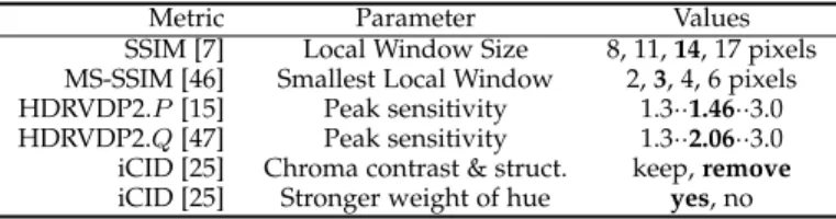
In order to fully explore their possibilities, we ran these metrics using different sets of parameters. For SSIM and MS-SSIM, we considered four sizes of local windows. HDR-VDP-2 is highly tunable: visual resolution, peak sensitivity, and surrounding luminance. For the resolution, we con-sidered 33.5 pixels per degree, which corresponds to our experimental setting, and we explored the peak sensitivity parameter within [1.3,3.0]. Surrounding luminance was set to the mean of the image, as this provided the best results. For these sets of parameters, we selected two kinds of output from HDR-VDP-2: the probability P of detection (we selected the mean and maximum values of the per-pixel probabilities, best results were provided by the mean), and the quality prediction Q proposed in the extension by Narwaria et al. [47]. For the iCID metric, we considered four versions by varying the weights of lightness, chroma, and hue, and by omitting or not, chroma contrast and chroma structure (as recommended by the authors). All these parameters are detailed in Table 4.

TABLE 4

Tested parameters of image quality metrics. Best parameter values (when testing on both datasets) appear in bold.

Metric Parameter Values SSIM [7] Local Window Size 8, 11, 14, 17 pixels MS-SSIM [46] Smallest Local Window 2, 3, 4, 6 pixels HDRVDP2.P[15] Peak sensitivity 1.3··1.46··3.0 HDRVDP2.Q[47] Peak sensitivity 1.3··2.06··3.0 iCID [25] Chroma contrast & struct. keep, remove iCID [25] Stronger weight of hue yes, no

5.2 Evaluation Measure

Our objective is to evaluate the performance of the metrics described above in predicting the perceived visibility of artifacts. This is a binary classification problem (i.e., visible or not visible), hence we evaluate the performance using the Receiver Operating Characteristic (ROC) curve, which represents the relation between sensitivity (true-positive rate) and specificity (true-negative rate) by varying a de-cision threshold on the metric output. The area under the ROC curve (AUC) can be used as a direct indicator of the performance (1.0 corresponds to a perfect classification, 0.5 corresponds to a random one). For each metric, instead of a single AUC value, we compute an AUC distribution using a bootstrap technique [48]: The AUC is computed 2000 times,

each time on a random set of images having the same size as the original dataset; this random set is generated by sampling with replacement. The bootstrap distribution allows for statistical testing and its percentiles provide the 95% confidence interval.

5.3 Performance Comparison on Rendered Images

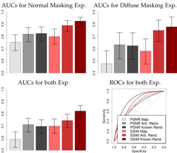
In this first study, image metrics are applied on rendered images. We evaluate the performance of the metrics on each dataset separately (resp. from normal masking and diffuse masking experiments) and on both datasets together (i.e., on all images). Figure 10 illustrates the AUC values for these three settings, and the ROC curve for the last one. The following sub-sections respectively present the performance of metrics and analyze their failures.

AUCs for Normal Masking Exp. AUCs for Diffuse Masking Exp.

AUCs for both Exp. ROCs for both Exp.

Fig. 10. AUC values (with95%confidence interval) for several image quality metrics applied on the rendered images. AUCs are computed on each dataset and on both together. ROC curves are also illustrated for this latter case. Metrics are represented by different colors detailed in the legend of the plots.

5.3.1 Overall Performance

When compression is applied on the diffuse texture (Nor-mal Masking Experiment), then SSIM provides the best performance, while not significantly better than MS-SSIM and iCID (P-value resp. equal to 0.10 and 0.58). In that case, HDR-VDP-2 (both Q and P ) performs significantly worse than its counterparts, except of course PSNR, which provides the worst results.

When compression is applied on the normal texture (Diffuse Masking Experiment), all metrics provide weaker perfor-mance, suggesting that compression artifacts applied on normal maps may be more difficult to predict. iCID provides the worst results, which is logical since it is based mostly on chrominance, while the normal map artifacts introduce mostly luminance impairments. MS-SSIM provides the best results, without being significantly different from SSIM and HDR-VDP-2.

Finally, when considering both datasets together, we chal-lenge the capability of metrics to generalize over different

artifacts. In that case, iCID, SSIM, and MS-SSIM show a statistically equivalent performance. However, ROC curves show that iCID is better on high specificity (i.e., low false-positive rate).

5.3.2 Analysis of Metric Failures

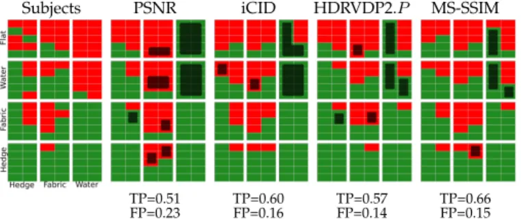
To understand more precisely the metric failures, we generated for each metric the classification results obtained at the Youden cut-point of the ROC curves, i.e., maximizing sensitivity + specificity. The obtained classifications are detailed in Figures 11 and 12 and their analysis is detailed below.

Normal Masking dataset. As can be seen in Figure 11, the PSNR metric completely underestimates the visibility of artifacts on the Water diffuse map, as compared with other maps. The reason is that this metric is unable to take into account the intrinsic masking effects inherent to the compressed texture content, which makes artifacts less visible when applied on a middle-high-frequency content (and thus more visible on low-frequency areas such as Water). HDR-VDP-2 and SSIM are better for this task but still tend to underestimate the visibility of Water artifacts for low compression strengths. We also observe that HDR-VDP-2 underestimates the effect of lighting for the Edge diffuse map, when strong maskers are present (Fabric and Edge). SSIM is slightly better for this task while PSNR completely fails. Note that iCID and MS-SSIM results are similar to SSIM’s, and VDP-2.Q is similar to HDR-VDP-2.P; their figures are available in the supplementary material.

Diffuse Masking dataset. For this dataset, once again, PSNR greatly underestimates the visibility of artifacts on the low-frequency Water normal map, while overestimates those from the high-frequency Fabric map. The iCID metric shares the same problem for this dataset. HDR-VDP-2 and SSIM better handle these intrinsic masking effects, however they still underestimate the Water artifacts for the 72◦ lighting. Note that for this dataset, SSIM results are similar to MS-SSIM’s, and VDP-2.Q is similar to HDR-VDP-2.P; their figures are available in the supplementary material.

Subjects PSNR HDRVDP2.P SSIM

TP=0.69, FP=0.17 TP=0.78, FP=0.13 TP=0.88, FP=0.16 Fig. 11. Classification obtained for different metrics at the maximum value of Youden’s index, for the Normal Masking experiment. Main differences w.r.t. the human-perceived classification are spotted in black.

Subjects PSNR iCID HDRVDP2.P MS-SSIM

TP=0.51 TP=0.60 TP=0.57 TP=0.66

FP=0.23 FP=0.16 FP=0.14 FP=0.15

Fig. 12. Classification obtained for different metrics at the maximum value of Youden’s index, for the Diffuse Masking experiment. Main differences w.r.t. the human-perceived classification are spotted in black.

5.4 Performance Comparison with Unknown Render-ing Parameters

In this section, we investigate how to predict the visual impact of artifacts, when the rendering parameters are un-known. This scenario corresponds to the most realistic use-case where the designer determines the compression level of the texture maps before any rendering and even without knowing the rendering parameters. In that case we consider two possibilities: either the metric is computed using only the compressed map (the masking map is ignored), or the metric is computed on a rendered image, with arbitrary light direction (in that case we selected a direction different from the images of the datasets). For comparison we also include results obtained when the metrics are computed on the rendered images from the datasets (as in the previous section). For this study, we consider the image metric that provided the best results in the study above, i.e., SSIM (with a 17 × 17 local window), as well as PSNR, commonly used by designers to evaluate and select the appropriate compression level. Figure 13 illustrates the results.

As can be seen in the figure, applying PSNR directly on the texture map provides a very poor prediction of the perceived visibility of artifacts (see the lightest-grey bars in the histograms). Applying SSIM directly on the texture map (lightest-red bars) is better but remains quite inefficient, especially for predicting artifacts from the normal maps (top right histogram). When the metrics are computed on rendered images with arbitrary light directions (medium-grey and medium-red bars), then results are much improved for both SSIM and PSNR. This implies that it is crucial to take into account the masking effects that occur during rendering, even in an approximate way (i.e., with arbitrary rendering parameters). As illustrated in the top row his-tograms, AUC values obtained when SSIM is computed on an arbitrary rendering (medium-red bars) are quite close to what is obtained when using the exact same render-ing parameters than in the psychophysical tests (dark-red bars). The difference between those two settings is larger when merging both datasets together (see bottom right histogram), meaning that it is more difficult to find a unique threshold on the metric outcome that will predict correctly the visibility of both diffuse and normal map compression artifacts.

AUCs for Normal Masking Exp. AUCs for Diffuse Masking Exp.

AUCs for both Exp. ROCs for both Exp.

Fig. 13. AUC values (with95%confidence intervals) for SSIM and PSNR applied on the texture maps (Map in the legend), on rendered images with arbitrary light directions (Arb. Rend.), and on the original rendered images from the experiments (Known Rend.). AUCs are computed on each dataset and on both together. ROC curves are also illustrated for this latter case. Metrics are represented by different colors detailed in the legend of the plots.

6

R

ECOMMENDATIONS AND DISCUSSION

Our analysis of artifact perceptual impacts (Sec. 4) and metric performance (Sec. 5) reveals several interesting findings and allows us to make useful recommendations for texture map compression.

First, Figures 7 and 9 illustrate that it is impossible to find a unique compression parameter for which artifacts remain invisible whatever the texture map. Indeed, even at the highest bit rate (i.e., smallest 6 × 6 block size), compression produces visible artifacts on certain texture maps when there is no masking. On the contrary, artifacts produced by the strongest compression (12 × 12) may be completely masked in some cases. So the conclusion that can be drawn here is that fixing the compression parameter to a single value for all texture maps is not a good way to proceed. It appears necessary to quantify the loss of quality due to compression.

As stated in the introduction, and as raised by Griffin and Olano [6], the most common approach in evaluating the quality loss due to texture compression is to use PSNR directly on the texture maps. However, as shown in Figure 13, it appears as a very bad strategy, since this process provides results close to random for predicting visibility of artifacts (see light-grey bars, AUC=0.60 when considering both datasets).

Figure 13 also shows that using a perceptual metric is far more efficient than PSNR, and in particular, SSIM (with the appropriate scale) provides the best results. As illustrated in Figure 13, like for PSNR, applying this perceptual metric directly on texture maps provides very bad results. The best way to predict the perceptual impact of artifacts is to apply this perceptual metric on rendered images. Since in most cases, the rendering parameters are not known beforehand, the metric could be applied on a simulated rendering using

an arbitrary light direction. The simplest way to proceed is to render both maps on a geometric square and then apply the perceptual metric on the resulting image. Such quick evaluation process, illustrated in the section below, can easily be integrated to a texture compression tool and would provide a significant improvement in visual quality estimation.

7

P

RACTICAL

A

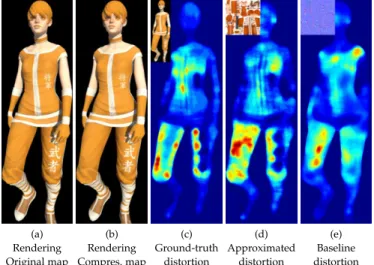
PPLICABILITY

To illustrate the process recommended above, we propose a practical application where we approximate the distor-tion present on a real 3D scene by running a metric on a simple rendering of a geometric square using an arbitrary light direction. We selected six 3D graphical assets (human characters) typical in games, which were put in a realistic pose, lit by sunlight and rendered using global illumination (see the first image in Figure 14). We applied either diffuse or normal texture compression using two strengths (10×10 and 12×12) and measured the ground-truth distortion maps using the SSIM metric on rendered images (see the third image in Figure 14). We then computed what we call the approximated distortion maps by running the SSIM metric on a geometric square mapped with both texture maps and lit by an arbitrary directional light (we selected three directions: 42◦, 27◦, and 13◦ from the normal direction of the square). We then texture mapped these approximated distortion maps onto the 3D object shapes (see the fourth image in Figure 14) and computed the correlation with the ground-truth distortion maps. In practice, we obtained 72 approximated maps (6 objects × 2 compression strengths × 2 compressed map types × 3 light directions). Note that correlations are computed over the rendered shapes only, and after median filtering to reduce noise. As baselines we applied the same process with distortion maps obtained by running the SSIM metric directly on the compressed texture maps (either diffuse or normal) without rendering, as illustrated in the fifth image in Figure 14.

Results are presented in Figure 15. More results are detailed in the supplementary material, together with all stimuli and distortion maps. We observe that the approximated distor-tion maps reach a mean correladistor-tion of 0.59 with the ground-truth distortion maps. This is reasonable and significantly better than results obtained by running the metric on the compressed maps alone (0.47 mean correlation). The per-formance of our approximation remains stable among light directions and reasonably stable among 3D shapes, whereas one asset led to significantly weaker results (Lumber, with a mean correlation of 0.41). Artifacts due to normal map compression appear more difficult to predict, than those due to diffuse map compression. The projection and shading on a real shape logically has a great impact on these artifacts as compared to our approximation on a geometric square.

Limitation. Precisely evaluating the perceptual impact of texture compression for an arbitrary 3D scene is highly complex, particularly when rendering parameters are not known beforehand. We showed that approximating the distortion using a flat Lambertian surface with an arbitrary directional lighting leads to improved and more stable results as compared to a baseline computation

(a) (b) (c) (d) (e) Rendering Rendering Ground-truth Approximated Baseline Original map Compres. map distortion distortion distortion Fig. 14. Illustration of the performance of our recommended distortion approximation. (a) Rendering of a 3D shape mapped with uncom-pressed diffuse and normal maps; (b) rendering after compression of the normal map (10×10); (c) ground-truth distortion obtained by computing the SSIM metric on the rendered images; (d) our approximation obtained by computing the metric after mapping diffuse and normal maps on a geometric square and rendering under a 13◦_{directional light (0.76}

correlation with ground-truth), and (e) baseline distortion obtained by computing the metric directly on the compressed normal map (0.54 correlation). At the top left of each distortion map, we display the image on which the distortion has been computed.

Effect of Approximated distortions Effect of light directions vs Baseline distortions on Approximated distortions

Effect of 3D shapes Effect of compressed map types on Approximated distortions on Approximated distortions

Fig. 15. Boxplots of Pearson correlations with ground-truth distortion. Top-left: Results obtained by Approximated and Baseline distortions (for all map types, lighting directions, and shapes). Other panels: Effects of the different factors on the Approximated distortions. Mean values are displayed as red circles.

on texture map only, i.e., a better ability to predict the real distortion that is caused by texture compression. An improved prediction would require to account for many additional factors: distortion due to projection on the 3D shape and foreshortening, self-visibility/occlusion over the surface, projected shadows and self-shadowing, non-uniform resolution of the texture map (in terms of texels per pixel), glossiness/”metalness” of material, silhouettes, inter-reflections, and much more complex light transport

of global illumination effects. Our findings constitute an important first step toward the full understanding of the perceptual impact of texture compression. Future work will explore all these factors to find improved ways to predict their effects without requiring the full rendering.

8

C

ONCLUSION

In this work, we presented a psychophysical experiment that investigates different masking effects in the percep-tion of texture compression artifacts. We show that strong compression artifacts can be hidden by contrast masking, while less severe artifacts may be visible when no masking occurs. We analysed how amplitude and frequency influ-ence masking effects and showed that these masking effects also depend on the interaction between diffuse and normal maps. Our analysis also emphasizes the significant impact of lighting in the perception of artifacts.

Our psychophysical data also allow us to evaluate the performance of image quality metrics in predicting the visibility of artifacts in different scenarios (on texture maps and on rendered images, with or without knowing the light direction) and to analyze their failures. We find that computing PSNR on texture maps is particularly inefficient and that a perceptual metric, such as SSIM, computed on a rendered image (even with an arbitrary lighting) provides much better performance.

Our dataset should stimulate research about visual quality metrics; indeed, even computed on a rendered image, we have shown that the best metrics are still far from reaching a perfect classification of visible distortions. In particular, the failures of the complex bottom-up HDR-VDP2 metric indicate that work is still needed to better predict human vision even in controlled condition. As raised by recent surveys [11], the future of quality metrics may rely on an appropriate combination of low-level psychophysical mod-els and machine learning techniques.

For compressing the texture we used the ASTC algorithm, which has the benefit of being random-access (i.e., each block of texture can be accessed and decompressed inde-pendently by the GPU) while being able to provide a large range of bit rates by varying the block size. Many other compression algorithms exist that may introduce different kinds of artifacts, depending on the transforms they use. For instance, the JPEG algorithm considers a fixed block size and quantizes Discrete Cosine Transform (DCT) coefficients. As part of future work, we would like to investigate the vari-ability of our results according to the nature of compression artifacts.

Finally, as stated in Sec. 3, we have considered texture maps corresponding to a traditional real-time shading workflow, where the diffuse texture contains not only the base color of the material but also some illumination effects (e.g., ambient occlusion, global illumination, etc.). We plan to make similar psychophysical studies with physically-based rendering (PBR) materials, i.e., represented for instance by albedo, ”metalness”, and roughness texture maps.

A

CKNOWLEDGMENT

This work was partly supported by Auvergne-Rhone-Alpes region under the COOPERA grant ”ComplexLoD”, by French National Research Agency as part of ANR-PISCo project (ANR-17-CE33-0005-01) and by the Natural Sciences and Engineering Research Council of Canada (NSERC).

R

EFERENCES

[1] D. S. Taubman and M. W. Marcellin, JPEG2000 Image Compression Fundamentals, Standards and Practice. Boston, MA: Springer US, 2002.

[2] J. Str ¨om and T. Akenine-M ¨oller, “i PACKMAN: high-quality, low-complexity texture compression for mobile phones,” ACM SIG-GRAPH/EUROGRAPHICS Conference on Graphics Hardware, pp. 177–182, 2005.

[3] J. Nystad, A. Lassen, A. Pomianowski, S. Ellis, and T. Olson, “Adaptive scalable texture compression,” ACM SIGGRAPH / Euro-graphics conference on High-Performance Graphics, pp. 105–114, 2012. [4] P. Krajcevski, “FasTC : Accelerated Fixed-Rate Texture Encoding,” in ACM SIGGRAPH Symposium on Interactive 3D Graphics and Games, 2013.

[5] M. Olano, D. Baker, W. Griffin, and J. Barczak, “Variable Bit Rate GPU Texture Decompression,” Computer Graphics Forum, vol. 30, no. 4, pp. 1299–1308, 2011.

[6] W. Griffin and M. Olano, “Evaluating Texture Compression Mask-ing Effects usMask-ing Objective Image Quality Assessment Metrics,” IEEE Transactions on Visualization and Computer Graphics, vol. 21, no. 8, pp. 970–979, 2015.

[7] Z. Wang, A. Bovik, H. Sheikh, and E. Simoncelli, “Image quality assessment: From error visibility to structural similarity,” IEEE Transactions on Image Processing, vol. 13, no. 4, pp. 600–612, 2004. [8] M. ˇCad´ık, R. Herzog, R. Mantiuk, K. Myszkowski, and H.-P.

Seidel, “New Measurements Reveal Weaknesses of Image Quality Metrics in Evaluating Graphics Artifacts,” ACM Transactions on Graphics, vol. 31, no. 6, pp. 147:1–147:10, 2012.

[9] G. Lavou´e, M.-C. Larabi, and L. Vasa, “On the Efficiency of Image Metrics for Evaluating the Visual Quality of 3D Models,” IEEE Transactions on Visualization and Computer Graphics, vol. 22, no. 8, pp. 1987–1999, Aug. 2016.

[10] J. Guo, V. Vidal, I. Cheng, A. Basu, A. Baskurt, and G. Lavou´e, “Subjective and Objective Visual Quality Assessment of Textured 3D Meshes,” ACM Transactions on Applied Perception, vol. 14, no. 2, pp. 11:1–11:20, Sep. 2016.

[11] G. Lavou´e and R. Mantiuk, “Quality assessment in computer graphics,” Visual Signal Quality Assessment: Quality of Experience (QoE), pp. 243–286, 2015.

[12] Z. Wang and A. C. Bovik, Modern Image Quality Assessment. Mor-gan & Claypool Publishers, Jan 2006.

[13] J. Lubin, “The use of psychophysical data and models in the analysis of display system performance,” in Digital Images and Human Vision, A. B. Watson, Ed., Oct 1993, pp. 163–178.

[14] S. Daly, “The visible differences predictor: an algorithm for the assessment of image fidelity,” in Digital images and human vision, Andrew B. Watson, Ed. Cambridge: MIT Press, oct 1993, pp. 179–206.

[15] R. Mantiuk, K. J. Kim, A. G. Rempel, and W. Heidrich, “Hdr-vdp-2: A calibrated visual metric for visibility and quality predictions in all luminance conditions,” ACM Transactions on Graphics, vol. 30, no. 4, pp. 40:1–40:14, Jul. 2011. [Online]. Available: http://doi.acm.org/10.1145/2010324.1964935

[16] M. Bolin and G. Meyer, “A perceptually based adaptive sampling algorithm,” in ACM Siggraph, 1998, pp. 299–309.

[17] K. Myszkowski, “The visible differences predictor: applications to global illumination problems,” in Rendering Techniques. Springer Vienna, 1998, pp. 223–236.

[18] M. Ramasubramanian, S. N. Pattanaik, and D. P. Greenberg, “A perceptually based physical error metric for realistic image syn-thesis,” in ACM Siggraph. ACM Press, 1999, pp. 73–82.

[19] M. Reddy, “SCROOGE: Perceptually-Driven Polygon Reduction,” Computer Graphics Forum, vol. 15, no. 4, pp. 191–203, 1996. [20] D. Luebke and B. Hallen, “Perceptually Driven Simplification

for Interactive Rendering,” in Eurographics Workshop on Rendering Techniques, 2001, pp. 223–234.

[21] L. Qu and G. Meyer, “Perceptually guided polygon reduction,” IEEE Transactions on Visualization and Computer Graphics, vol. 14, no. 5, pp. 1015–1029, 2008.

[22] N. Menzel and M. Guthe, “Towards Perceptual Simplification of Models with Arbitrary Materials,” Computer Graphics Forum, vol. 29, no. 7, pp. 2261–2270, Sep 2010.

[23] H. Sheikh and A. Bovik, “Image information and visual quality,” IEEE Transactions on Image Processing, vol. 15, no. 2, pp. 430–444, Feb 2006.

[24] L. Zhang, X. Mou, and D. Zhang, “FSIM: A Feature Similarity Index for Image Quality Assessment.” IEEE Transactions on Image Processing, no. 99, pp. 2378–2386, jan 2011.

[25] J. Preiss, F. Fernandes, and P. Urban, “Color-image quality assess-ment: From prediction to optimization,” IEEE Transactions on Image Processing, vol. 23, no. 3, pp. 1366–1378, 2014.

[26] Y. Liu and J. Wang, “A No-Reference Metric for Evaluating the Quality of Motion Deblurring,” in SIGGRAPH Asia, 2013. [27] F. Gao, D. Tao, S. Member, and X. Gao, “Learning to Rank for

Blind Image Quality Assessment,” IEEE Trans. on Neural Networks and Learning Systems, pp. 1–30, 2015.

[28] H. Yeganeh and Z. Wang, “Objective quality assessment of tone-mapped images,” IEEE Transactions on Image Processing, vol. 22, no. 2, pp. 657–667, 2013.

[29] Q. Zhu, J. Zhao, Z. Du, and Y. Zhang, “Quantitative analysis of discrete 3D geometrical detail levels based on perceptual metric,” Computers & Graphics, vol. 34, no. 1, pp. 55–65, Feb 2010.

[30] A. Brady, J. Lawrence, P. Peers, and W. Weimer, “genBRDF: Dis-covering New Analytic BRDFs with Genetic Programming,” ACM Transactions on Graphics, vol. 33, no. 4, pp. 1–11, 2014.

[31] V. Havran, J. Filip, and K. Myszkowski, “Perceptually Motivated BRDF Comparison using Single Image,” Computer Graphics Forum, vol. 35, no. 4, pp. 1–12, 2016.

[32] T. O. Aydin, M. ˇCad´ık, K. Myszkowski, and H.-P. Seidel, “Video quality assessment for computer graphics applications,” ACM Transactions on Graphics, vol. 29, no. 6, pp. 161:1–161:12, dec 2010. [33] R. Herzog, M. Cadik, T. O. Aydin, K. I. Kim, K. Myszkowski,

and H.-p. Seidel, “NoRM : No-Reference Image Quality Metric for Realistic Image Synthesis,” Computer Graphics Forum, vol. 31, no. 2, pp. 545–554, 2012.

[34] M. ˇCad´ık, R. Herzog, R. Mantiuk, R. Mantiuk, K. Myszkowski, and H.-P. Seidel, “Learning to Predict Localized Distortions in Rendered Images,” in Pacific Graphics, vol. 32, no. 7, 2013. [35] G. Lavou´e, “A Multiscale Metric for 3D Mesh Visual Quality

Assessment,” Computer Graphics Forum, vol. 30, no. 5, pp. 1427– 1437, 2011.

[36] L. V´aˇsa and J. Rus, “Dihedral Angle Mesh Error: a fast percep-tion correlated distorpercep-tion measure for fixed connectivity triangle meshes,” Computer Graphics Forum, vol. 31, no. 5, pp. 1715–1724, 2012.

[37] M. Corsini, E. D. Gelasca, T. Ebrahimi, and M. Barni, “Water-marked 3-D Mesh Quality Assessment,” IEEE Transactions on Multimedia, vol. 9, no. 2, pp. 247–256, Feb 2007.

[38] Y. Pan, I. Cheng, and A. Basu, “Quality metric for approximating subjective evaluation of 3-D objects,” IEEE Transactions on Multi-media, vol. 7, no. 2, pp. 269–279, Apr 2005.

[39] J. Filip, M. J. Chantler, P. R. Green, and M. Haindl, “A psychophys-ically validated metric for bidirectional texture data reduction,” ACM Transactions on Graphics, vol. 27, no. 5, p. 1, dec 2008. [40] M. Guthe, G. M ¨uller, M. Schneider, and R. Klein, “BTF-CIELab:

A Perceptual Difference Measure for Quality Assessment and Compression of BTFs,” Computer Graphics Forum, vol. 28, no. 1, pp. 101–113, Mar 2009.

[41] A. Jarabo, H. Wu, J. Dorsey, H. Rushmeier, and D. Gutierrez, “Effects of approximate filtering on the appearance of bidirectional texture functions,” IEEE Transactions on Visualization and Computer Graphics, vol. 20, no. 6, pp. 880–892, 2014.

[42] A. R. Rao and G. L. Lohse, “Towards a texture naming system: Identifying relevant dimensions of texture,” in Vision Research, 1996, vol. 36, no. 11, pp. 1649–1669.

[43] ARM Mali, “GPU Texture Compression Tool.” [Online]. Available: https://developer.arm.com/products/software-development-tools/graphics-development-tools/mali-texture-compression-tool [44] NVIDIA, “Mental Ray.” [Online]. Available:

http://www.nvidia.fr/object/nvidia-mental-ray-fr.html

[45] L. Zhang, “A comprehensive evaluation of full reference image quality assessment algorithms,” in International Conference on Image Processing (ICIP), 2012, pp. 1477–1480.

[46] Z. Wang, E. Simoncelli, and A. Bovik, “Multiscale structural sim-ilarity for image quality assessment,” in IEEE Asilomar Conference on Signals, Systems and Computers, 2003, pp. 1398–1402.

[47] M. Narwaria, R. K. Mantiuk, M. P. Da Silva, and P. Le Callet, “HDR-VDP-2.2: a calibrated method for objective quality pre-diction of high-dynamic range and standard images,” Journal of Electronic Imaging, vol. 24, no. 1, p. 010501, 2015.

[48] B. Efron and R. Tibshirani, An Introduction to the Bootstrap. Chap-man & Hall/CRC Monographs on Statistics & Applied Probability, 1993.

Guillaume Lavou ´e (M’11-SM’13) received his PhD from the University of Lyon (2005) where he is now an associate professor. He defended his habilitation title in 2013. His research interests include diverse aspects of geometry processing as well as quality assessment and perception for computer graphics. Guillaume Lavoue authored more than 30 journal papers and has been chair-ing the IEEE SMC TC on Human Perception and Multimedia Computing (2013-2017). He serves as an associate editor for The Visual Computer journal.

Michael Langer is an Associate Professor in the School of Computer Science and a member of the Centre for Intelligent Machines at McGill Uni-versity. He received a B.Sc. in Mathematics from McGill in 1986, M.Sc. in Computer Science from the University of Toronto in 1988, and Ph.D. from McGill in 1994. He was a postdoctoral fellow at the NEC Research Institute in Princeton NJ, and a Humboldt Research Fellow at the Max-Planck-Institute for Biological Cybernetics in Tuebingen, Germany. He has been a professor at McGill since 2000.

Adrien Peytavie is an Assistant Professor of Computer Science at the University of Lyon, France. He received a PhD in Computer Science from University Claude Bernard Lyon 1 in Com-puter Science in 2010. His research interests in-clude procedural modeling of virtual worlds and simulating natural phenomena.

Pierre Poulin is a full professor and chair of the department of Computer Science and Op-erations Research at the Universit ´e de Montr ´eal. He holds a Ph.D. from the University of British Columbia and an M.Sc. from the University of Toronto, both in Computer Science. He has served on more than 60 program committees of international conferences. He has supervised 15 Ph.D. and more than 40 M.Sc. students. His research interests cover a wide range of topics, including image synthesis, image-based model-ing, procedural modelmodel-ing, natural phenomena, scientific visualization, and computer animation.