Construction of Dependent Dirichlet
Processes Based on Poisson Processes
The MIT Faculty has made this article openly available.
Please share
how this access benefits you. Your story matters.
Citation
D. Lin et al. "Construction of Dependent Dirichlet Processes based
on Poisson Processes" Neural Information Processing Systems
2010.
As Published
http://nips.cc/Conferences/2010/Program/accepted-papers.php
Publisher
Neural Information Processing Systems Foundation (NIPS)
Version
Author's final manuscript
Citable link
http://hdl.handle.net/1721.1/73948
Terms of Use
Creative Commons Attribution-Noncommercial-Share Alike 3.0
Construction of Dependent Dirichlet Processes
based on Poisson Processes
Dahua Lin CSAIL, MIT [email protected] Eric Grimson CSAIL, MIT [email protected] John Fisher CSAIL, MIT [email protected]
Abstract
We present a method for constructing dependent Dirichlet processes. The new ap-proach exploits the intrinsic relationship between Dirichlet and Poisson processes in order to create a Markov chain of Dirichlet processes suitable for use as a prior over evolving mixture models. The method allows for the creation, removal, and location variation of component models over time while maintaining the property that the random measures are marginally DP distributed. Additionally, we derive a Gibbs sampling algorithm for model inference and test it on both synthetic and real data. Empirical results demonstrate that the approach is effective in estimating dynamically varying mixture models.
1
Introduction
As the corner stone of Bayesian nonparametric modeling, Dirichlet processes (DP) [22] have been widely used in solving a variety of inference and estimation problems [3, 10, 20]. One of the most successful application are Dirichlet process mixtures (DPM) [15, 17], which are a generalization of finite mixture models that allow an indefinite number of mixture components. Traditional DPMs assume that each sample is generated independently from the same DP, which limits its utility, as in many cases different samples may come from different yet dependent DPs. While HDPs [23] provide a way to construct multiple DPs implicitly depending on each other via a common parent, their hierarchical structure may not be appropriate in some problems (e.g. temporally varying DPs). Consider a topic model where each document is generated under a particular topic, and each topic is characterized by a distribution over words. Over time, topics change: some old topics fade while new ones emerge. For each particular topic, the word distribution may evolve as well. A natural approach to model such topics is to use a Markov chain of DPs as a prior, such that the DP at each time is generated by varying the previous one in three possible ways: creating a new topic, removing an existing topic, and changing the word distribution of a topic.
Since MacEachern introduced the notion of dependent Dirichlet processes (DDP) [12], a vari-ety of DDP constructions have been developed, which are based on either weighted mixtures of DPs [6, 14, 18], generalized Chinese restaurant processes [4, 21, 24], or the stick breaking construc-tion [5, 7]. Here, we propose a fundamentally different approach, taking advantage of the intrinsic relations between Dirichlet processes and Poisson processes: a Dirichlet process is a normalized Gamma process, while a Gamma process is essentially a compound Poisson process.The key idea is motivated by the observation that applying an operation that preserves complete randomness to Poisson processes will result in a new process that remains Poisson. Therefore, one can obtain a Dirichlet process depending on other DPs by applying such operations to their underlying compound Poisson processes. In particular, we discuss three types of operations: superposition, subsampling, and point transition. We develop a Markov chain of DPs by combining these operations, leading to a framework that allows creation, removal, and location variation of particles. This construction inherently comes with an elegant property that the random measure at each time is marginally DP
distributed. Our approach relates to previous efforts in constructing dependent DPs while overcom-ing inherent limitations. A detailed comparison is given in section 4.
2
Poisson, Gamma, and Dirichlet Processes
Our construction of dependent Dirichlet processes is based on the connections between Poisson, Gamma, and Dirichlet processes, as well as the concept of completely randomness. Here, we briefly review these concepts. See Kingman [9] for a detailed exposition of the relevant theory.
Let (Ω, FΩ) be a measurable space, and Π be a random point process on Ω. Each realization of Π uniquely corresponds to a counting measure NΠdefined by NΠ(A) := #(Π ∩ A) for each A ∈ FΩ. Hence, NΠis a measure-valued random variable or simply a random measure. A Poisson process Π on Ω with mean measure µ, denoted Π ∼ PoissonP(µ), is defined to be a point process such that NΠ(A) has a Poisson distribution with mean µ(A) and that for any disjoint measurable sets A1, . . . , An, NΠ(A1), . . . , NΠ(An) are independent. The latter property is referred to as complete randomness. Poisson processes are the only point process that satisfies this property [9]:
Theorem 1. A random point process Π on a regular measure space is a Poisson process if and only ifNΠis completely random. If this is true, the mean measure is given byµ(A) = E(NΠ(A)). Consider Π∗ ∼ PoissonP(µ∗
) on a product space Ω × R+. For each realization of Π∗, We define Σ∗: FΩ→ [0, +∞] as
Σ∗:= X (θ,wθ)∈Π∗
wθδθ (1)
Intuitively, Σ∗(A) sums up the values of wθwith θ ∈ A. Note that Σ∗is also a completely random measure (but not a point process in general), and it is essentially a generalization of the compound Poisson process. As a special case, if we choose µ∗to be
µ∗= µ × γ with γ(dw) = w−1e−wdw, (2) Then the random measure as defined in Eq.(1) is called a Gamma process with base measure µ, denoted by G ∼ ΓP(µ). Normalizing any realization of G ∼ ΓP(µ) yields a sample of a Dirichlet process, as
D := G/G(Ω) ∼ DP(µ). (3)
In conventional parameterization, µ is often decomposed into two parts: a base distribution pµ := µ/µ(Ω), and a concentration parameter αµ:= µ(Ω).
3
Construction of Dependent Dirichlet Processes
Motivated by the relations between Poisson processes and Dirichlet processes, we develop a new approach of constructing dependent Dirichlet processes (DDPs). In a high level, our approach can be described as follows. Given a collection of Dirichlet processes, we can apply operations that preserve complete randomness to their underlying Poisson processes, which would yield a new Poisson process (due to theorem 1), and thus a new DP depending on the source. In particular, we study three such operations: superposition, subsampling, and point transition.
Superposition of Poisson processes: Combining a set of independent Poisson processes yields a Poisson process whose mean measure is the sum of mean measures of the individual ones.
Theorem 2 (Superposition Theorem [9]). Let Π1, . . . , Πmbe independent Poisson processes onΩ withΠk∼ PoissonP(µk), then their union has
Π1∪ · · · ∪ Πm ∼ PoissonP(µ1+ · · · + µm). (4) Given a collection of independent Gamma processes G1, . . . , Gm, where for each k = 1, . . . , m, Gk∼ ΓP(µk) with underlying Poisson process Π∗k ∼ PoissonP(µk× γ). By theorem 2, we have
m [ k=1 Π∗k ∼ PoissonP m X k=1 (µk× γ) ! = PoissonP m X k=1 µk ! × γ ! . (5)
According to the relation between Gamma processes and their underlying Poisson processes, such combination is tantamount to directly superimposing the Gamma processes themselves, as
G0 := G1+ · · · + Gm∼ ΓP(µ1+ · · · + µm). (6) Let Dk = Gk/Gk(Ω), and gk = Gk(Ω), then Dk is independent of gk, and thus
D0 := G0/G0(Ω) = (g1D1+ · · · + gmDm)/(g1+ · · · + gm) = c1D1+ · · · + cmDm. (7) Here, ck = gk/P
m
l=1gl, which has (c1, . . . , cm) ∼ Dir(µ1(Ω), . . . , µm(Ω)). Consequently, one can construct a Dirichlet process through a random convex combination of independent Dirichlet processes. This result is summarized by the following theorem:
Theorem 3. Let D1, . . . , Dm be independent Dirichlet processes onΩ with Dk ∼ DP(µk), and (c1, . . . , cm) ∼ Dir(µ1(Ω), . . . , µm(Ω)) be independent of D1, . . . , Dm, then
D1⊕ · · · ⊕ Dm:= c1D1+ · · · cmDm ∼ DP(µ1+ · · · + µm). (8) Here, we use the symbol ⊕ to indicate superposition via a random convex combination. Let αk = µk(Ω) and α0 =Pmk=1αk, then for each measurable subset A,
E(D0(A)) = m X
k=1 αk
α0E(Dk(A)), and Cov(D 0(A), D
k(A)) = αk
α0Var(Dk(A)). (9) Subsampling Poisson processes: Random subsampling of a Poisson process via independent Bernoulli trials yields a new Poisson process.
Theorem 4 (Subsampling Theorem). Let Π ∼ PoissonP(µ) be a Poisson process on the space Ω, andq : Ω → [0, 1] be a measurable function. If we independently draw zθ∈ {0, 1} for each θ ∈ Π0 with P(zθ = 1) = q(θ), and let Πk = {θ ∈ Π : zθ = k} for k = 0, 1, then Π0 andΠ1 are independent Poisson processes onΩ, with Π0∼ PoissonP((1 − q)µ) and Π1∼ PoissonP(qµ)1. We emphasize that subsampling is via independent Bernoulli trials rather than choosing a fixed number of particles. We use Sq(Π) := Π1to denote the result of subsampling, where q is referred to as the acceptance function. Note that subsampling the underlying Poisson process of a Gamma process G is equivalent to subsampling the terms of G. Let G =P∞
i=1wiδθi, and for each i, we
draw ziwith P(zi= 1) = q(θi). Then, we have G0 = Sq(G) :=
X
i:zi=1
wiδθi ∼ ΓP(qµ). (10)
Let D be a Dirichlet process given by D = G/G(Ω), then we can construct a new Dirichlet pro-cess D0 = G0/G0(Ω) by subsampling the terms of D and renormalizing their coefficients. This is summarized by the following theorem.
Theorem 5. Let D ∼ DP(µ) be represented by D =Pn
i=1riδθiandq : Ω → [0, 1] be a
measur-able function. For eachi we independently draw ziwith P(zi= 1) = q(θi), then D0 = Sq(D) :=
X
i:zi=1
r0iδθi ∼ DP(qµ), (11)
whereri0 := ri/Pj:zj=1rjare the re-normalized coefficients for thosei with zi= 1.
Let α = µ(Ω) and α0 = (qµ)(Ω), then for each measurable subset A, E(D0(A)) = (qµ)(A) (qµ)(Ω) = R Aqdµ R Ωqdµ
, and Cov(D0(A), D(A)) =α 0 αVar(D
0(A)). (12)
Point transition of Poisson processes: The third operation moves each point independently fol-lowing a probabilistic transition. Formally, a probabilistic transition is defined to be a function T : Ω × FΩ→ [0, 1] such that for each θ ∈ FΩ, T (θ, ·) is a probability measure on Ω that describes the distribution of where θ moves, and for each A ∈ FΩ, T (·, A) is integrable. T can be considered as a transformation of measures over Ω, as
(T µ)(A) := Z
Ω
T (θ, A)µ(dθ). (13)
1qµ is a measure on Ω given by (qµ)(A) =R
Theorem 6 (Transition Theorem). Let Π ∼ PoissonP(µ) and T be a probabilistic transition, then T (Π) := {T (θ) : θ ∈ Π} ∼ PoissonP(T µ). (14) With a slight abuse of notation, we useT (θ) to denote an independent sample from T (θ, ·). As a consequence, we can derive a Gamma process and thus a Dirichlet process by applying the probabilistic transition to the location of each term, leading to the following:
Theorem 7. Let D =P∞
i=1riδθi ∼ DP(µ) be a Dirichlet process on Ω, then
T (D) := ∞ X
i=1
riδT (θi) ∼ DP(T µ). (15)
Theorems 1 and 2 are immediate consequences of the results in [9]. Theorem 3 to Theorem 7 are derived in developing the proposed approach. Detailed explanation of relevant concepts and the proofs of theorem 2 to theorem 7 are provided in the supplement.
3.1 A Markov Chain of Dirichlet Processes
Integrating these three operations, we construct a Markov chain of DPs formulated as
Dt= T (Sq(Dt−1)) ⊕ Ht, with Ht∼ DP(ν). (16) The model can be explained as follows: given Dt−1, we choose a subset of terms by subsampling, then move their locations via a probabilistic transition T , and finally superimpose a new DP Hton the resultant process to form Dt. Hence, creating new particles, removing existing particles, and varying particle locationsare all allowed, respectively, via superposition, subsampling, and point transition. Note that while they are based on the operations of the underlying Poisson processes, due to theorems 3, 5, and 7, we operate directly on the DPs, without the need of explicitly instantiating the associated Poisson processes or Gamma processes. Let µtbe the base measure of Dt, then
µt= T (qµt−1) + ν. (17)
Particularly, if the acceptance probability q is a constant, then αt= qαt−1+ αν. Here, αt= µt(Ω) and αν = ν(Ω) are the concentration parameters. One may hold αt fixed over time by choosing appropriate values for q and αν. Furthermore, it can be shown that
Cov(Dt+n(A), Dt(A)) ≤ qnVar(Dt(A)). (18) The covariance with a previous DPs decays exponentially when q < 1. This is often a desirable property in practice. Moreover, we note that ν and q play different roles in controlling the process. Generally, ν determines how frequently a new terms appear; while q governs the the life span of a term which has a geometric distribution with mean (1 − q)−1.
We aim to use the Markov chain of DPs as a prior of evolving mixture models. This provides a mechanism with which new component models can be brought in, existing components can be removed, and the model parameters can vary smoothly over time.
4
Comparison with Related Work
In his pioneering work [12], MacEachern proposed the “single-p DDP model”. It considers DDP as a collection of stochastic processes, but does not provide a natural mechanism to change the collection size over time. M¨uller et al [14] formulated each DP as a weighted mixture of a common DP and an independent DP. This formulation was extended by Dunson [6] in modeling latent trait distributions. Zhu et al [24] presented the Time-sensitive DP, in which the contribution of each DP decays exponentially. Teh et al [23] proposed the HDP where each child DP takes its parent DP as the base measure. Ren [18] combines the weighted mixture formulation with HDP to construct the dynamic HDP. In contrast to the model proposed here, a fundamental difference of these models is that the marginal distribution at each node is generally not a DP.
Caron et al [4] developed a generalized Polya Urn scheme while Ahmed and Xing [1] developed the recurrent Chinese Restaurant process (CRP). Both generalize the CRP to allow time-variation, while
retaining the property of being marginally DP. The motivation underlying these methods fundamen-tally differs from ours, leading to distinct differences in the sampling algorithm. In particular, [4] supports innovation and deletion of particles, but does not support variation of locations. Moreover, its deletion scheme is based on the distribution in history, but not on whether a component model fits the new observation. While [1] does support innovation and point transition, there is no explicit way to delete old particles. It can be considered a special case of the proposed framework in which subsampling operation is not incorporated. We note that [1] is motivated from an algorithmic rather than theoretical perspective.
Grifin and Steel [7] present the πDDP based on the stick breaking construction [19], reordering the stick breaking ratios for each time so as to obtain different distributions over the particles. This work is further extended [8] to a generic stick breaking processes. Chung et al [5] propose a local DP that generalizes πDDP. Rather than reordering the stick breaking ratios, they regroup them locally such that dependent DPs can be constructed over a general covariate space. Inference in these mod-els requires sampling a series of auxiliary variables, considerably increasing computational costs. Moreover, the local DP relies on a truncated approximation to devise the sampling scheme. Recently, Rao and Teh [16] proposed the spatially normalized Gamma process. They constructs a universal Gamma process in an auxiliary space and obtain dependent DPs by normalizing it within overlapped local regions. The theoretical foundation differs in that it does not exploit the relations between Gamma process and Poisson process which is in the heart of the proposed model. In [16], the dependency is established through region overlapping; while in our work, this is accomplished by explicitly transferring particles from one DP to another. In addition, this work does not support location variation, as it relies on a universal particle pool that is fixed over time.
5
The Sampling Algorithm
We develop a Gibbs sampling procedure based on the construction of DDP introduced above. The key idea is to derive the sampling steps by exploiting the fact that our construction maintains the property of being marginally DP via connections to the underlying Poisson processes. Furthermore, the derived procedure unifies distinct aspects (innovation, removal, and transition) of our model. Let D ∼ DP(µ) be a Dirichlet process on Ω. Then given a set of samples Φ ∼ D, in which φiappears citimes, we have D|Φ ∼ DP(µ + c1δφ1+ · · · + cnδφn). Let D
0be a Dirichlet process depending on D as in Eq.(16), α0= (qµ)(Ω), and qi= q(θi). Given Φ ∼ D, we have
D0|Φ ∼ DP ανpν+ α0pqµ+ m X k=1 qkckT (φk, ·) ! . (19)
Sampling from D0. Let θ1∼ D0. Marginalizing over D0, we get θ1|Φ ∼ αν α01pν+ α0 α01pqµ+ m X k=1 qkck α01 T (φk, ·) with α 0 1= αν+ α0+ m X k=1 qkck. (20) Thus we sample θ1from three types of sources: the innovation distribution pν, the q-subsampled base distribution pqµ, and the transition distribution T (φk, ·). In doing so, we first sample a variable u1that indicates which source to sample from. Specifically, when u1= −1, u1= 0, or u1= l > 0, we respectively sample θ1 from pν, pqµ, or T (φl, ·). The probabilities of these cases are αν/α01, α0/α01, and qici/α01respectively. After u1is obtained, we then draw θ1from the indicated source. The next issue is how to update the posterior given θ1andu1. The answer depends on the value of u1. When u1= −1 or 0, θ1is a new particle, and we have
D0|θ1, {u1≤ 0} ∼ DP ανpν+ α0pqµ+ m X k=1 qkckT (φk, ·) + δθ1 ! . (21)
If u1 = l > 0, we know that the particle φlis retained in the subsampling process (i.e. the corre-sponding Bernoulli trial outputs 1), and the transited version T (φl) is determined to be θ1. Hence,
D0|θ1, {u1= l > 0} ∼ DP ανpν+ α0pqµ+ X k6=l qkckT (θk, ·) + (cl+ 1)δθ1 . (22)
With this posterior distribution, we can subsequently draw the second sample and so on. This process generalizes the Chinese restaurant process in several ways: (1) it allows either inheriting previous particles or drawing new ones; (2) it uses qkto control the chance that we sample a previous particle; (3) the transition T allows smooth variation when we inherit a previous particle.
Inference with Mixture Models. We use the Markov chain of DPs as the prior of evolving mixture models. The generation process is formulated as
θ1, . . . , θn∼ D0 i.i.d., and xi∼ L(θi), i = 1, . . . , n. (23) Here, L(θi) is the observation model parameterized by θi. According to the analysis above, we derive an algorithm to sample θ1, . . . , θnconditioned on the observations x1, . . . , xnas follows. Initialization. (1) Let ˜m denote the number of particles, which is initialized to be m and will increase as we draw new particles from pνor pqµ. (2) Let wkdenote the prior weights of different sampling sources which may also change during the sampling. Particularly, we set wk = qkck for k > 0, w−1 = αν, and w0 = α0. (3) Let ψkdenote the particles, whose value is decided when a new particle or the transited version of a previous one is sampled. (4) The label liindicates to which particle θicorresponds and the counter rk records the number of times that ψk has been sampled (set to 0 initially). (5) We compute the expected likelihood, as given by F (k, i) := Epk(f (xi|θ)).
Here, f (xi|θ) is the likelihood of xjwith respect to the parameter θ, and pk is pν, pqµor T (φk, ·) respectively when k = −1, k = 0 and k ≥ 1.
Sequential Sampling. For each i = 1, . . . , n, we first draw the indicator uiwith probability P(ui= k) ∝ wkF (k, i). Depending on the value of ui, we sample θifrom different sources. For brevity, let p|x to denote the posterior distribution derived from the prior distribution p conditioned on the observation x. (1) If ui = −1 or 0, we draw θifrom pν|xior pqµ|xi, respectively, and then add it as a new particle. Concretely, we increase ˜m by 1, let ψm˜ = θj, rm˜ = wm˜ = 1, and set li = ˜m. Moreover, we compute F (m, i) = f (xi|ψm˜) for each i. (2) Suppose ui = k > 0. If rk= 0 then it is the first time we have drawn ui= k. Since ψkhas not been determined, we sample θi∼ T (φk, ·)|xi, then set ψk = θi. If rk > 0, the k-th particle has been sampled before. Thus, we can simply set θi= ψk. In both cases, we set the label li= k, increase the weight wiand the counter riby 1, and update F (k, i) to f (xi|ψk) for each i.
Note that this procedure is inefficient in that it samples each particle φk merely based on the first observation with label k. Therefore, we use this procedure for bootstrapping, and then run a Gibbs sampling scheme that iterates between parameter update and label update.
(Parameter update): We resample each particle ψk from its source distribution conditioned on all samples with label k. In particular, for k ∈ [1, m] with rk > 0, we draw ψk ∼ T (φk, ·)|{xi : li= k}, and for k ∈ [m + 1, ˜m], we draw ψk∼ p|{xi: li= k}, where p = pqµor pν, depending which source ψk was initially sampled from. After updating ψk, we need to update F (k, i) accordingly. (Label update): The label updating is similar to the bootstrapping procedure described above. The only difference is that when we update a label from k to k0, we need to decrease the weight and counter for k. If rkdecreases to zero, we remove ψk, and reset wkto qkckwhen k ≤ m.
At the end of each phase t, we sample ψk ∼ T (φk, ·) for each k with rk = 0. In addition, for each of such particles, we update the acceptance probability as qk ← qk· q(φk), which is the prior probability that the particle φk will survive in next phase. MATLAB codes are available in the following website: http://code.google.com/p/ddpinfer/.
6
Experiments
Here we present experimental results on both synthetic and real data. In the synthetic case, we compare both methods in modeling mixtures of Gaussians whose number and centers evolve over time. For real data, we test the approach in modeling the motion of people in crowded scenes and the trends of research topics reflected in index terms.
6.1 Simulations on Synthetic Data
The data for simulations were synthesized as follows. We initialized the model with two Gaussian components, and added new components following a temporal Poisson process (one per 20 phases
0 10 20 30 40 50 60 70 80 0 0.05 0.1 0.15 0.2 median distance D−DPMM D−FMM (K = 2) D−FMM (K = 3) D−FMM (K = 5) 0 10 20 30 40 50 60 70 80 0 5 t actual # comp.
(a) Comparison with D-FMM
0 50 100 150 200 0 0.05 0.1 0.15 0.2 # samples/component median distance q=0.1 q=0.9 q=1
(b) For different acceptance prob.
0 50 100 150 200 0 0.1 0.2 0.3 0.4 0.5 0.6 0.7 0.8 # samples/component median distance var=0.0001 var=0.1 var=100
(c) For different diffusion var.
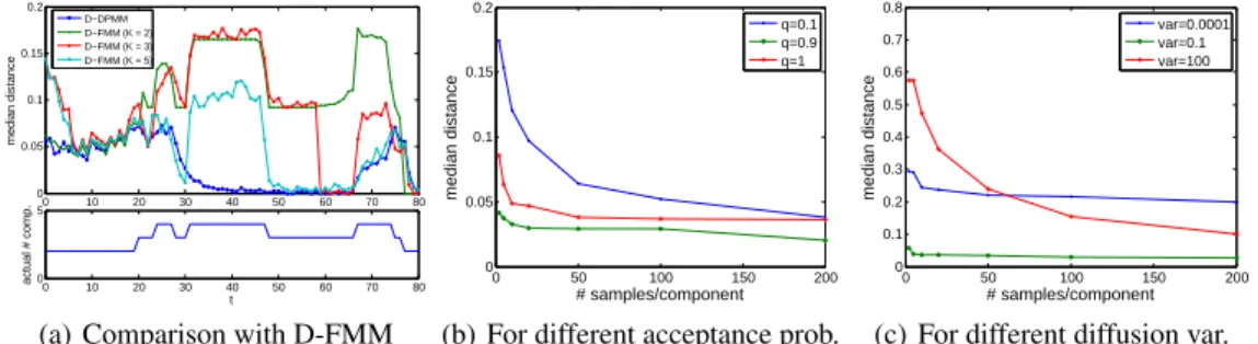
Figure 1:The simulation results: (a) compares the performance between D-DPMM and D-FMM with differing numbers of components. The upper graph shows the median of distance between the resulting clusters and the ground truth at each phase. The lower graph shows the actual numbers of clusters. (b) shows the performance of D-DPMM with different values of acceptance probability, under different data sizes. (c) shows the performance of D-DPMM with different values of diffusion variance, under different data sizes.
on average). For each component, the life span has a geometric distribution with mean 40, the mean evolves independently as a Brownian motion, and the variance is fixed to 1. We performed the simulation for 80 phases, and at each phase, we drew 1000 samples for each active component. At each phase, we sample for 5000 iterations, discarding the first 2000 for burn-in, and collecting a sample for every 100 iterations for performance evaluation. The particles of the last iteration at each phase were incorporated into the model as a prior for sampling in the next phase. We obtained the label for each observation by majority voting based on the collected samples, and evaluated the performance by measuring the dissimilarity between the resultant clusters and the ground truth using the variation of information [13]. Under each parameter setting, we repeated the experiment for 20 times, utilizing the median of the dissimilarities for comparison.
We compare our approach (D-DPMM) with dynamic finite mixtures (D-FMM), which assumes a fixed number of Gaussians whose centers vary as Brownian motion. From Figure 1(a), we observe that when the fixed number K of components equals the actual number, they yield comparable per-formance; while when they are not equal, the errors of D-FMM substantially increase. Particularly, K less than the actual number results in significant underfitting (e.g. D-FMM with K = 2 or 3 at phases 30 − 50 and 66 − 76); when K is greater than the actual number, samples from the same com-ponent are divided into multiple groups and assigned to different comcom-ponents (e.g. D-FMM with K = 5 at phases 1 − 10 and 30 − 50). In all cases, D-DPMM consistently outperforms D-FMM due to its ability to adjust the number of components to adapt to the change of observations.
We also studied how design parameters impact performance. In Figure 1(b), we see that setting the acceptance probability q to 0.1 tends to create new components rather than inheriting from previous phases, leading to poor performance when the number of samples is limited. If we set q = 0.9, the components in previous phase have more chance survive, and thus the estimation of the component parameter can be based on multiple phases, which is more reliable. Figure 1(c) shows the effect of the diffusion variance that controls the parameter variation. When it is small, the parameter in next phase is tied tightly with the previous value; when it is large, the estimation basically relies on new observations. Both cases lead to performance degradation on small datasets, which indicates that it is important to keep a balance between inheritance and innovation. Our framework provides the flexibility to attain such balance. Cross-validation can be used to set these parameters automatically. 6.2 Real Data Applications
Modeling People Flows. It was observed [11] that the majority of people walking in crowded areas such as a rail station tend to follow motion flows. Typically, there are several flows at a time, and each flow may last for a period. In this experiment, we apply our approach to extract the flows. The test was conducted on a video acquired in New York Grand Central Station (provided by the author of [11]), which comprises 90, 000 frames for one hour (25 fps). A low level tracker was used to obtain the tracks of people, which were then processed by a rule-based filter that discards obviously incorrect tracks. We adopt the flow model described in [11], which uses an affine field to capture the motion patterns of each flow. The observation for this model is in form of location-velocity
0 10 20 30 40 50 60 0 2 4 6 8 10 12 14 16 18 20 time index flow 1 flow 2 (a) People flows
1990 1995 2000 2005 2010 0 1 2 3 4 5 6 7 8 9 10 11 time index
1 motion estimation, video sequences
2 pattern recognition, pattern clustering
3 statistical models, optimization problem
4 discriminant analysis, information theory
5 image segmentation, image matching
6 face recognition, biological
7 image representation, feature extraction
8 photometry, computational geometry
9 neural nets, decision theory
10 image registration, image color analysis
(b) PAMI topics
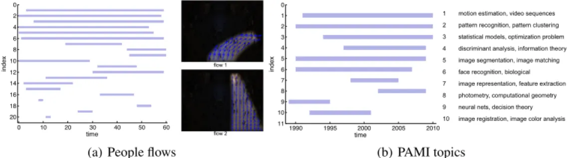
Figure 2:The experiment results on real data. (a) left: the timelines of the top 20 flows; right: illustration of first two flows. (Illustrations of larger sizes are in the supplement.) (b) left: the timelines of the top 10 topics; right: the two leading keywords for these topics. (A list with more keywords is in the supplement.)
pairs. We divided the entire sequence into 60 phases (each for one minute), extract location-velocity pairs from all tracks, and randomly choose 3000 pairs for each phase for model inference. The algorithm infers 37 flows in total, while at each phase, the numbers of active flows range from 10 to 18. Figure 2(a) shows the timelines of the top 20 flows (in terms of the numbers of assigned observations). We compare the performance of our method with D-FMM by measuring the average likelihood on a disjoint dataset. The value for our method is −3.34, while those for D-FMM are −6.71, −5.09, −3.99, −3.49, and −3.34, when K are respectively set to 10, 20, 30, 40, and 50. This shows that with much smaller number of components (12 active components on average), our method can attain similar modeling accuracy as a D-FMM with 50 components.
Modeling Paper Topics. Next we analyze the evolution of paper topics for IEEE Trans. on PAMI. By parsing the webpage of IEEE Xplore, we collected the index terms for 3014 papers published in PAMI from Jan, 1990 to May, 2010. We first compute the similarity between each pair of papers in terms of relative fraction of overlapped index terms. We derive a 12-dimensional feature vector using spectral embedding [2] over the similarity matrix for each paper. We run our algorithm on these features with each phase corresponding to a year. Each cluster of papers is deemed a topic. We compute the histogram of index terms and sorted them in decreasing order of frequency for each topic. Figure 2(b) shows the timelines of top 10 topics, and together with the top two index terms for each of them. Not surprisingly, we see that topics such as “neural networks” arise early and then diminish while “image segmentation” and “motion estimation” persist.
7
Conclusion and Future Directions
We developed a principled framework for constructing dependent Dirichlet processes. In contrast to most DP-based approaches, our construction is motivated by the intrinsic relation between Dirichlet processes and compound Poisson processes. In particular, we discussed three operations: super-position, subsampling, and point transition, which produce DPs depending on others. We further combined these operations to derive a Markov chain of DPs, leading to a prior of mixture models that allows creation, removal, and location variation of component models under a unified formula-tion. We also presented a Gibbs sampling algorithm for inferring the models. The simulations on synthetic data and the experiments on modeling people flows and paper topics clearly demonstrate that the proposed method is effective in estimating mixture models that evolve over time.
This framework can be further extended along different directions. The fact that each completely random point process is a Poisson process suggests that any operation that preserves the complete randomness can be applied to obtain dependent Poisson processes, and thus dependent DPs. Such operations are definitely not restricted to the three ones discussed in this paper. For example, random merging and random splitting of particles also possess this property, which would lead to an extended framework that allows merging and splitting of component models. Furthermore, while we focused on Markov chain in this paper, the framework can be straightforwardly generalized to any acyclic network of DPs. It is also interesting to study how it can be generalized to the case with undirected network or even continuous covariate space. We believe that as a starting point, this paper would stimulate further efforts to exploit the relation between Poisson processes and Dirichlet processes.
References
[1] A. Ahmed and E. Xing. Dynamic Non-Parametric Mixture Models and The Recurrent Chinese Restaurant Process : with Applications to Evolutionary Clustering. In Proc. of SDM’08, 2008.
[2] F. R. Bach and M. I. Jordan. Learning spectral clustering. In Proc. of NIPS’03, 2003. [3] J. Boyd-Graber and D. M. Blei. Syntactic Topic Models. In Proc. of NIPS’08, 2008.
[4] F. Caron, M. Davy, and A. Doucet. Generalized Polya Urn for Time-varying Dirichlet Process Mixtures. In Proc. of UAI’07, number 6, 2007.
[5] Y. Chung and D. B. Dunson. The local Dirichlet Process. Annals of the Inst. of Stat. Math., (October 2007), January 2009.
[6] D. B. Dunson. Bayesian Dynamic Modeling of Latent Trait Distributions. Biostatistics, 7(4), October 2006.
[7] J. E. Griffin and M. F. J. Steel. Order-Based Dependent Dirichlet Processes. Journal of the American Statistical Association, 101(473):179–194, March 2006.
[8] J. E. Griffin and M. F. J. Steel. Time-Dependent Stick-Breaking Processes. Technical report, 2009. [9] J. F. C. Kingman. Poisson Processes. Oxford University Press, 1993.
[10] J. J. Kivinen, E. B. Sudderth, and M. I. Jordan. Learning Multiscale Representations of Natural Scenes Using Dirichlet Processes. In Proc. of ICCV’07, 2007.
[11] D. Lin, E. Grimson, and J. Fisher. Learning Visual Flows: A Lie Algebraic Approach. In Proc. of CVPR’09, 2009.
[12] S. N. MacEachern. Dependent Nonparametric Processes. In Proceedings of the Section on Bayesian Statistical Science, 1999.
[13] M. Meila. Comparing clusterings - An Axiomatic View. In Proc. of ICML’05, 2005.
[14] P. Muller, F. Quintana, and G. Rosner. A Method for Combining Inference across Related Nonparametric Bayesian Models. J. R. Statist. Soc. B, 66(3):735–749, August 2004.
[15] R. M. Neal. Markov Chain Sampling Methods for Dirichlet Process Mixture Models. Journal of compu-tational and graphical statistics, 9(2):249–265, 2000.
[16] V. Rao and Y. W. Teh. Spatial Normalized Gamma Processes. In Proc. of NIPS’09, 2009. [17] C. E. Rasmussen. The Infinite Gaussian Mixture Model. In Proc. of NIPS’00, 2000.
[18] L. Ren, D. B. Dunson, and L. Carin. The Dynamic Hierarchical Dirichlet Process. In Proc. of ICML’08, New York, New York, USA, 2008. ACM Press.
[19] J. Sethuraman. A Constructive Definition of Dirichlet Priors. Statistica Sinica, 4(2):639–650, 1994. [20] K.-a. Sohn and E. Xing. Hidden Markov Dirichlet process: modeling genetic recombination in open
ancestral space. In Proc. of NIPS’07, 2007.
[21] N. Srebro and S. Roweis. Time-Varying Topic Models using Dependent Dirichlet Processes, 2005. [22] Y. W. Teh. Dirichlet Process, 2007.
[23] Y. W. Teh, M. I. Jordan, M. J. Beal, and D. M. Blei. Hierarchical Dirichlet Processes. Journal of the American Statistical Association, 101(476):1566–1581, 2006.