Mathematics for Business Science and Technology with MATLAB and Excel pdf - Web Education

(1)

M T

H

A

Mathematics

for Business, Science, and Technology

with MATLAB ® and Excel ® Computations

Third Edition

Steven T. Karris x y 10 0 20 0 30 0 4 00 50 0 2,0 00 4,0 00 6 ,0 00 8,0 00 1 0,00 0 0 Unit s Sold 12 ,00 0 1 4,00 0 Revenue Cos t B reak-Even P oint Profit $

Includes a

Comprehensive Treatment of Probability and Statistics Illustrated

with Numerous Examples

Orchard Publications

(2)

Mathematics for Business, Science, and Technology with MATLAB® and Excel® Computations, Third Edition Copyright © 2007 Orchard Publications. All rights reserved. Printed in the United States of America. No part of this publication may be reproduced or distributed in any form or by any means, or stored in a data base or retrieval system, without the prior written permission of the publisher.

Direct all inquiries to Orchard Publications, 39510 Paseo Padre Parkway, Fremont, California 94538, U.S.A. URL: http://www.orchardpublications.com, e-mail:info@orchardpublications.com.

Product and corporate names are trademarks or registered trademarks of the MathWorks™, Inc., and Microsoft™ Corporation. They are used only for identification and explanation, without intent to infringe.

Library of Congress Cataloging-in-Publication Data

Library of Congress Control Number: 2007922089 Copyright Number TX-5-471-563

ISBN-13: 978-1-934404-01-0 ISBN-10: 1-934404-01-2 Disclaimer

The publisher has used his best effort to prepare this text. However, the publisher and author makes no warranty of any kind, expressed or implied with regard to the accuracy, completeness, and computer codes contained in this book, and shall not be liable in any event for incidental or consequential damages in connection with, or arising out of, the performance or use of these programs.

(3)

1

Elementary Algebra 1−1 1.1 Introduction...1−1 1.2 Algebraic Equations...1−2 1.3 Laws of Exponents...1−5 1.4 Laws of Logarithms...1−10 1.5 Quadratic Equations...1−13 1.6 Cubic and Higher Degree Equations...1−15 1.7 Measures of Central Tendency...1−15 1.8 Interpolation and Extrapolation...1−20 1.9 Infinite Sequences and Series...1−23 1.10 Arithmetic Series...1−23 1.11 Geometric Series...1−24 1.12 Harmonic Series ...1−26 1.13 Proportions ...1−27 1.14 Summary...1−29 1.15 Exercises ...1−33 1.16 Solutions to End−of−Chapter Exercises ...1−35 Excel Computations: Pages 1−7, 1−11, 1−16, 1−17, 1−33, 1−36

MATLAB Computations: Pages 1−7, 1−11

2

Intermediate Algebra 2−1

2.1 Systems of Two Equations ... 2−1 2.2 Systems of Three Equations... 2−6 2.3 Matrices and Simultaneous Solution of Equations... 2−7 2.4 Summary ... 2−26 2.5 Exercises... 2−30 2.6 Solutions to End−of−Chapter Exercises ...2−32 Excel Computations: Pages 2−23, 2−24, 2−30, 2−31

MATLAB Computations: Pages 2−15, 2−16, 2−24, 2−25, 2−32, 2−36

3

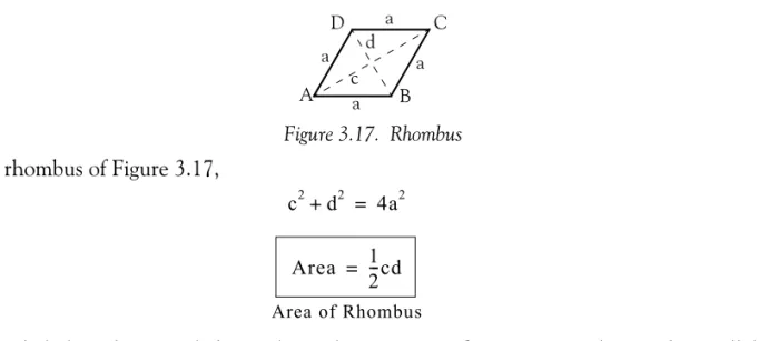
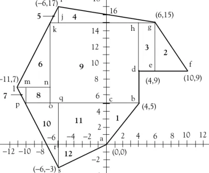
Fundamentals of Geometry 3−1

3.1 Introduction...3−1 3.2 Plane Geometry Figures...3−1 3.3 Solid Geometry Figures...3−16 3.4 Using Spreadsheets to Find Areas of Irregular Polygons...3−20 3.5 Summary...3−23

(4)

7

0

0 +

+

D

V

D

’

s

F

O

R

S

A

L

E

&

E

X

C

H

A

N

G

E

w

ww

w

.

t

ra

r

ad

de

er

rs

s-

-s

so

o

ft

f

t

wa

w

ar

r

e

.c

.

co

o

m

w

.

f

o

r

e

x

-

w

a

r

e

z

.

c

o

m

w

ww

w.

.

tr

t

r

ad

a

di

in

ng

g

-s

-

so

o

ft

f

tw

wa

ar

r

e-

e

-c

c

ol

o

ll

le

e

c

ti

t

io

o

n

.

c

o

m

w

.

t

r

a

d

e

s

t

a

t

i

o

n

-

d

o

w

n

l

o

a

d

-

f

r

e

.

c

o

m

C

o

n

t

a

c

t

s

a

n

d

r

e

y

b

r

v

@

g

m

a

i

l

.

c

o

m

a

n

d

r

e

y

b

r

v

@

y

a

n

d

e

x

.

r

u

S

k

y

p

e

:

a

n

d

r

e

y

b

r

v

(5)

3.6 Exercises... 3−27 3.7 Solutions to End−of−Chapter Exercises... 3−29 Excel Computations: Pages 3−20, 3−30

4

Fundamentals of Plane Geometry 4−1

4.1 Introduction... 4−1 4.2 Trigonometric Functions... 4−2 4.3 Trigonometric Functions of an Acute Angle... 4−2 4.4 Trigonometric Functions of an Any Angle ... 4−3 4.5 Fundamental Relations and Identities ... 4−6 4.6 Triangle Formulas... 4−12 4.7 Inverse Trigonometric Functions ... 4−13 4.8 Area of Polygons in Terms of Trigonometric Functions... 4−14 4.9 Summary... 4−16 4.10 Exercises ... 4−18 4.11 Solutions to End−of−Chapter Exercises ... 4−19

Excel Computations: Pages 4−9 through 4−11, 4−13, 4−19 through 4−21 MATLAB Computations: Page 4−15

5

Fundamentals of Calculus 5−1

5.1 Introduction... 5−1 5.2 Differential Calculus ... 5−1 5.3 The Derivative of a Function ... 5−3 5.4 Maxima and Minima... 5−11 5.5 Integral Calculus... 5−15 5.6 Indefinite Integrals... 5−16 5.7 Definite Integrals ... 5−16 5.8 Summary ... 5−21 5.9 Exercises... 5−23 5.10 Solutions to End−of−Chapter Exercises ... 5−24 Excel Computations: Pages 5−8, 5−11, 5−18

MATLAB Computations: Pages 5−24 through 5−26

6

Mathematics of Finance and Economics 6−1 6.1 Common Terms... 6−1 6.1.1 Bond... 6−1 6.1.2 Corporate Bond ... 6−1 6.1.3 Municipal Bond ... 6−1

(6)

6.1.4 Treasury Bond ... 6−1 6.1.5 Perpetuity ... 6−1 6.1.6 Perpetual Bond... 6−1 6.1.7 Convertible Bond ... 6−2 6.1.8 Treasury Note ... 6−2 6.1.9 Treasury Bill ... 6−2 6.1.10 Face Value ... 6−2 6.1.11 Par Value... 6−2 6.1.12 Book Value... 6−3 6.1.13 Coupon Bond... 6−3 6.1.14 Zero Coupon Bond ... 6−3 6.1.15 Junk Bond... 6−3 6.1.16 Bond Rating Systems... 6−3 6.1.17 Promissory Note ... 6−4 6.1.18 Discount Rate... 6−4 6.1.19 Prime Rate ... 6−4 6.1.20 Mortgage Loan ... 6−4 6.1.21 Predatory Lending Practices... 6−5 6.1.22 Annuity ... 6−5 6.1.23 Ordinary Annuity... 6−5 6.1.24 Sinking Fund ... 6−6 6.2 Interest ... 6−6 6.2.1 Simple Interest... 6−6 6.2.2 Compound Interest... 6−8 6.2.3 Effective Interest Rate ... 6−22 6.3 Sinking Funds... 6−24 6.4 Annuities... 6−29 6.5 Amortization ... 6−34 6.6 Perpetuities... 6−36 6.7 Valuation of Bonds... 6−39 6.7.1 Calculating the Purchase Price of a Bond... 6−40 6.7.2 Total Periodic Bond Disbursement... 6−42 6.7.3 Calculation of Interest Rate of Bond ... 6−44 6.8 Spreadsheet Financial Functions ... 6−45 6.8.1 PV Function ... 6−46 6.8.2 FV Function ... 6−48 6.8.3 PMT Function... 6−49 6.8.4 RATE Function... 6−50 6.8.5 NPER Function... 6−51 6.8.6 NPV Function ... 6−52 6.8.7 IIR Function... 6−54

(7)

6.8.8 MIIR Function... 6−56 6.8.9 IPMT Function... 6−58 6.8.10 PPMT Function ... 6−59 6.8.11 ISPMT Function... 6−60 6.9 The MATLAB Financial Toolbox ... 6−61 6.9.1 irr MATLAB Function... 6−61 6.9.2 effrr MATLAB Function... 6−62 6.9.3 pvfix MATLAB Function ... 6−62 6.9.4 pvvar MATLAB Function ... 6−63 6.9.5 fvfix MATLAB Function ... 6−64 6.9.6 fvvar MATLAB Function ... 6−65 6.9.7 annurate MATLAB Function...6−66 6.9.8 amortize MATLAB Function ...6−67 6.10 Comparison of Alternate Proposals ...6−68 6.11 Kelvin’s Law...6−71 6.12 Summary ...6−75 6.13 Exercises...6−78 6.14 Solutions to End−of−Chapter Exercises ...6−81 Excel Computations: Pages 6−10 through 6−14, 6−28, 6−29, 6−33, 6−35,

6−45 through 6−52, 6−54, 6−56, 6−58 through 6−61, 6−81 MATLAB Computations: Pages 6−61, 6−68

7

Depreciation, Impairment, and Depletion 7−1 7.1 Depreciation Defined... 7−1 7.1.1 Items that Can Be Depreciated ... 7−2 7.1.2 Items that Cannot Be Depreciated ... 7−2 7.1.3 Depreciation Rules... 7−2 7.1.4 When Depreciation Begins and Ends ... 7−3 7.1.5 Methods of Depreciation ... 7−3 7.1.5.1 Straight−Line (SL) Depreciation Method... 7−4 7.1.5.2 Sum of the Years Digits (SYD) Method ... 7−5 7.1.5.3 Fixed-Declining Balance (FDB) Method ... 7−6 7.1.5.4 The 125%, 150%, and 200% General Declining Balance Methods... 7−8 7.1.5.5 The Variable Declining Balance Method... 7−9 7.1.5.6 The Units of Production Method ... 7−10 7.1.5.7 Depreciation Methods for Income Tax Reporting ... 7−11 7.2 Impairments... 7−18 7.3 Depletion ... 7−19 7.4 Valuation of a Depleting Asset ... 7−20 7.5 Summary... 7−25

(8)

7.6 Exercises ...7−27 7.7 Solutions to End−of−Chapter Exercises...7−28

Excel Computations: Pages 7−4, 7−6, 7−7, 7−9, 7−10, 7−29 through 7−32 MATLAB Computations: Pages 7−30, 7−31, 7−33

8

Introduction to Probability and Statistics 8−1 8.1 Introduction ...8−1 8.2 Probability and Random Experiments ...8−1 8.3 Relative Frequency ...8−2 8.4 Combinations and Permutations ...8−4 8.5 Joint and Conditional Probabilities...8−7 8.6 Bayes’ Rule ...8−11 8.7 Summary ...8−13 8.8 Exercises...8−15 8.9 Solutions to End−of−Chapter Exercises...8−16 Excel Computations: Pages 8−6, 8−16

9

Random Variables 9−1

9.1 Definition of Random Variables...9−1 9.2 Probability Function ...9−2 9.3 Cumulative Distribution Function...9−2 9.4 Probability Density Function...9−9 9.5 Two Random Variables ...9−11 9.6 Statistical Averages ...9−12 9.7 Summary...9−20 9.8 Exercises ...9−23 9.9 Solutions to End−of−Chapter Exercises ...9−24 Excel Computations: Page 9−3

10

Common Probability Distributions and Tests of Significance 10−1 10.1 Properties of Binomial Coefficients ...10−1 10.2 The Binomial (Bernoulli) Distribution...10−2 10.3 The Uniform Distribution ...10−6 10.4 The Exponential Distribution ...10−10 10.5 The Normal (Gaussian) Distribution ...10−12 10.6 Percentiles...10−32 10.7 The Student’s t−Distribution ...10−36 10.8 The Chi−Square Distribution...10−40

(9)

10.9 The F Distribution ... 10−43 10.10 Chebyshev’s Inequality ... 10−46 10.11 Law of Large Numbers ... 10−46 10.12 The Poisson Distribution ... 10−47 10.13 The Multinomial Distribution ... 10−52 10.14 The Hypergeometric Distribution ... 10−53 10.15 The Bivariate Normal Distribution ... 10−56 10.16 The Rayleigh Distribution ... 10−56 10.17 Other Probability Distributions ... 10−59 10.17.1 The Cauchy Distribution... 10−59 10.17.2 The Geometric Distribution ... 10−59 10.17.3 The Pascal Distribution... 10−59 10.17.4 The Weibull Distribution... 10−60 10.17.5 The Maxwell Distribution... 10−61 10.17.6 The Lognormal Distribution ... 10−61 10.18 Critical Values of the Binomial Distribution ... 10−62 10.19 Sampling Distribution of Means ... 10−63 10.20 Z −Score ... 10−64 10.21 Tests of Hypotheses and Levels of Significance... 10−65 10.22 Tests of Significance... 10−72 10.22.1 The z−Test ... 10−72 10.22.2 The t−Test ... 10−73 10.22.3 The F−Test... 10−74 10.22.4 The Chi−SquareTest... 10−75 10.23 Summary... 10−80 10.24 Exercises... 10−89 10.24 Solutions to End−of−Chapter Exercises... 10−91 Excel Computations: Pages 10−28, 10−29, 10−35, 10−36, 10−39, 10−40, 10−43,

10−45, 10−51, 10−55, 10−60, 10−62, 10−69 through 10−75, 10−77, 10−78, 10−93, 10−95

MATLAB Computations: Pages 10−21, 10−28, 10−31, 10−32, 10−37, 10−41

11

Curve Fitting, Regression, and Correlation 11−1 11.1 Curve Fitting ... 11−1 11.2 Linear Regression ... 11−2 11.3 Parabolic Regression ... 11−7 11.4 Covariance ... 11−10 11.5 Correlation Coefficient ... 11−12 11.6 Summary ... 11−17 11.7 Exercises... 11−20

(10)

11.8 Solutions to End−of−Chapter Exercises ...11−22 Excel Computations: Pages 11−3, 11−4, 11−6, 11−7, 11−8, 11−11 through 11−13,

11−15, 11−22 through 11−25

12

Analysis of Variance (ANOVA) 12−1

12.1 Introduction...12−1 12.2 One−way ANOVA...12−1 12.3 Two−way ANOVA...12−8 12.3.1 Two−factor without Replication ANOVA... 12−8 12.3.2 Two−factor with Replication ANOVA...12−14 12.4 Summary ...12−25 12.5 Exercises...12−29 12.6 Solutions to End−of−Chapter Exercises ...12−31 Excel Computations: Pages 12−6 through 12−8, 12−13, 12−14, 12−22 through 12−24,

12−31, 12−33, 12−35, 12−37

A

Numbers and Arithmetic Operations A−1

A.1 Number Systems...A−1 A.2 Positive and Negative Numbers...A−1 A.3 Addition and Subtraction ...A−2 A.4 Multiplication and Division ...A−7 A.5 Integer, Fractional, and Mixed Numbers...A−10 A.6 Reciprocals of Numbers ...A−11 A.7 Arithmetic Operations with Fractional Numbers...A−13 A.8 Exponents...A−22 A.9 Scientific Notation...A−25 A.10 Operations with Numbers in Scientific Notation...A−27 A.11 Square and Cubic Roots...A−30 A.12 Common and Natural Logarithms ...A−32 A.13 Decibel ...A−33 A.14 Percentages...A−34 A.15 International System of Units (SI)...A−35 A.16 Graphs ...A−40 A.17 Summary...A−44 A.18 Exercises ...A−50 A.19 Solutions to End−of−Appendix Exercises...A−51

Excel Computations: Pages A−13 through A−18, A−26, A−30 through A−35, A−37, A−39, A−51

(11)

B

Introduction to MATLAB® B−1

B.1 MATLAB® and Simulink®... B−1 B.2 Command Window ... B−1 B.3 Roots of Polynomials ... B−3 B.4 Polynomial Construction from Known Roots ... B−4 B.5 Evaluation of a Polynomial at Specified Values... B−5 B.6 Rational Polynomials... B−8 B.7 Using MATLAB to Make Plots ... B−10 B.8 Subplots ... B−18 B.9 Multiplication, Division, and Exponentiation ... B−18 B.10 Script and Function Files ... B−26 B.11 Display Formats ... B−31 MATLAB Computations: Entire Appendix

C

The Gamma and Beta Functions and Distributions C−1 C.1 The Gamma Function ...C−1 C.2 The Gamma Distribution ...C−15 C.3 The Beta Function ...C−17 C.4 The Beta Distribution ...C−20 Excel Computations: Pages C−5, C−11, C−16, C−17, C−19

MATLAB Computations: Pages C−3 through C−5, C−10, C−16, C−19, C−20

D

Introduction to Markov Chains D−1

D.1 Stochastic Processes... D−1 D.2 Stochastic Matrices... D−1 D.3 Transition Diagrams ... D−4 D.4 Regular Stochastic Matrices ... D−5 D.5 Some Practical Examples ... D−7 Excel Computations: Pages D−8, D−11, D−14

E

The Lambda Index E−1

E.1 Introduction ... E−1 E.2 The Lambda Index Defined... E−1

(12)

E.3 Spreadsheet Construction ...E−2 Excel Computations: Page E−2

F

The Black−Scholes Stock Options Model F−1 F.1 Stock Options ... F−1 F.2 The Black-Scholes Model Equations ... F−2 F.3 Spreadsheet for the Black−Scholes Model... F−3 Excel Computations: Page F−3

G

Forecasting Bankruptcy G−1

G.1 The Financial Ratios...G−1 G.2 Interpretation of The Altman Z−Score...G−2 G.3 Spreadsheet for The Altman Z−Score...G−2 Excel Computations: Page G−2

References R−1

(13)

Preface

This text is written for

a. high school graduates preparing to take business or science courses at community colleges or universities

b. working professionals who feel that they need a math review from the very beginning

c. young students and working professionals who are enrolled in continued education institutions, and majoring in business related topics, such as business administration and accounting, and those pursuing a career in science, electronics, and computer technology. Chapter 1 is an introduction to the basics of algebra.

Chapter 2 is a continuation of Chapter 1 and presents some practical examples with systems of two and three equations.

Chapters 3 and 4 discuss the fundamentals of geometry and trigonometry respectively. These treatments are not exhaustive; these chapters contain basic concepts that are used in science and technology.

Chapter 5 is an abbreviated, yet a practical introduction to calculus.

Chapters 6 and 7 serve as an introduction to the mathematics of finance and economics and the concepts are illustrated with numerous real−world applications and examples.

Chapters 8 through 12 are devoted to probability and statistics. Many practical examples are given to illustrate the importance of this branch of mathematics. The topics that are discussed, are especially important in management decisions and in reliability. Some readers may find certain topics hard to follow; these may be skipped without loss of continuity.

In all chapters, numerous examples are given to teach the reader how to obtain quick answers to some complicated problems using computer tools such as MATLAB®and Microsoft Excel.® Appendix A contains a review of the basic arithmetic operations, introduces the SI system of units, and discusses different types of graphs. It is written for the reader who needs a review of the very basics of arithmetic.

Appendix B is intended to teach the interested reader how to use MATLAB. Many practical examples are presented. The Student Edition of MATLAB is an inexpensive software package; it can be found in many college bookstores, or can be obtained directly from

(14)

The MathWorks™ Inc., 3 Apple Hill Drive, Natick, MA 01760−2098 Phone: 508 647−7000, Fax: 508 647−7001

http://www.mathworks.com e−mail: info@mathwork.com

Appendix C introduces the gamma and beta functions. These appear in the gamma and beta distributions and find many applications in business, science, and engineering. For instance, the Erlang distributions, which are a special case of the gamma distribution, form the basis of queuing theory.

Appendix D is an introduction to Markov chains. A few practical examples illustrate their application in making management decisions.

Appendices E, F, and G are introductions to the Lambda Index, Black−Scholes stock options pricing, and the Altman Z−score bankruptcy prediction respectively.

Every chapter and appendix in this text is supplemented with Excel and / or MATLAB scripts to verify the computations and to construct relevant plots. The pages where the Excel and MATLAB scripts appear are listed in the Table of Contents.

New to the Second Edition

This is an refined revision of the first edition. The most notable changes are the addition of the new Chapters 6 and 7, chapter−end summaries, and detailed solutions to all exercises. The latter is in response to many students and working professionals who expressed a desire to obtain the author’s solutions for comparison with their own.

New to the Third Edition

This is an refined revision of the second edition. The most notable is the addition of Appendices E, F, and G. All chapters and Appendices A through D have been rewritten, and graphs have been redrawn with the latest MATLAB® Student Version, Release 14.

All feedback for typographical errors and comments will be most welcomed and greatly appreciated.

Orchard Publications

www.orchardpublications.com info@orchardpublications.com

(15)

Chapter 1 Elementary Algebra

his chapter is an introduction to algebra and algebraic equations. A review of the basic arithmetic concepts is provided in Appendix A. It also introduces some financial functions that are used with Excel. Throughout this text, a left justified horizontal bar will denote the beginning of an example, and a right justified horizontal bar will denote the end of the example. These bars will not be shown whenever an example begins at the top of a page or at the bottom of a page. Also, when one example follows immediately after a previous example, the right justified bar will be omitted.

1.1 Introduction

Algebra is the branch of mathematics in which letters of the alphabet represent numbers or a set of

numbers. Equations are equalities that indicate how some quantities are related to others. For example, the equation

(1.1) is a relation or formula that enables us to convert degrees Fahrenheit, , to degrees Celsius, . For instance, if the temperature is , the equivalent temperature in is

We observe that the mathematical operation in parentheses, that is, the subtraction of from

, was performed first. This is because numbers within parentheses have precedence (priority)

over other operations.

In algebra, the order of precedence, where is the highest and is the lowest, is as follows: 1. Quantities inside parentheses ( )

2. Exponentiation

3. Multiplication and Division 4. Addition or Subtraction

T

°C = 5₉---(_{°F 32}– ) °F °C 77°F °C °C 5 9 --- 77 32( – ) 5 9 --- 45× 25 = = = 32 77 1 4

(16)

Chapter 1 Elementary Algebra

Example 1.1

Simplify the expression

Solution:

This expression is reduced in steps as follows:

Step 1. Subtracting from inside the parentheses yields . Then, Step 2. Performing the exponentiation operations we get

Step 3. Multiplying by we get

Step 4. Dividing by we get (Simplest form)

An equality is a mathematical expression where the left side is equal to the right side. For example,

is an equality since the left and right sides are equal to each other.

1.2 Algebraic Equations

An algebraic equation is an equality that contains one or more unknown quantities, normally repre-sented by the last letters of the alphabet such as , , and . For instance, the expressions , , and are algebraic equations. In the last two equations, the multiplication sign between and and and is generally omitted; thus, they are written as and . Henceforth, terms such as will be interpreted as , as , and, in general, as .

Solving an equation means finding the value of the unknown quantity that will make the equation an equality with no unknowns. The following properties of algebra enable us to find the numerical value of the unknown quantity in an equation.

Property 1

The same number may be added to, or subtracted from both sides of an equation.

a –23 8 3– ( )2×4 ---= 3 8 5 a –23 52×4 ---= a –8 25 4× ---= 25 4 a –8 100 ---= 8 – 100 a = –0.08 7 3+ = 10 x y z x 5+ = 15 3 y× = 24 x y× = 12 3 y x y 3y = 24 xy = 12 3y 3 y× xy x y× XY X Y×

(17)

Algebraic Equations

Example 1.2

Given the equality

prove that Property 1 holds if we a. add to both sides

b. subtract from both sides Proof:

a. Adding to both sides we get

or and thus, the equality holds.

b. Subtracting from both sides we get

or and thus, the equality holds.

Example 1.3

Solve the following equation, that is, find the value of . Solution:

We need to find a value for so that the equation will still hold after the unknown has been replaced by the value that we have found. For this type of equations, a good approach is to find a number that when added to or subtracted from both sides of the equation, the left side will con-tain only the unknown . For this example, this will be accomplished if we add to both sides of the given equation. When we do this, we get

and after simplification, we obtain the value of the unknown x as

We can check this answer by substitution of into the given equation. Thus, or . Therefore, our answer is correct.

7 5+ = 12 3 2 3 7 5 3+ + = 12 3+ 15 = 15 2 7 5 2+ – = 12 2– 10 = 10 x x 5– = 15 x x x 5 x 5– +5 = 15 5+ x = 20 x 20 5– = 15 15 = 15

(18)

Chapter 1 Elementary Algebra

Example 1.4

Solve the following equation, that is, find the value of . Solution:

Again, we need to find a number such that when added to or subtracted from both sides of the equation, the left side will have the unknown only. In this example, this will be accomplished if we subtract 5 from both sides of the given equation. Doing this, we get

and after simplification, we obtain the value of the unknown as

To verify that this is the correct answer, we substitute this value into the given equation and we

get or .

Property 2

Each side of an equation can be multiplied or divided* by the same number.

Example 1.5

Solve the following equation, that is, find the value of .

(1.2) Solution:

We need to eliminate the denominator on the left side of the equation. This is done by multi-plying both sides of the equation by . Then,

and after simplification we get

(1.3) To verify that this is correct, we divide by ; this yields , and this is equal to the right side of

* Division by zero is meaningless; therefore, it must be avoided.

x x 5+ = 15 x x 5 5+ – = 15 5– x x = 10 10 5+ = 15 15 = 15 y y 3 --- = 24 3 3 y 3 --- 3× = 24 3× y = 72 72 3 24

(19)

Laws of Exponents

the given equation. Note 1.1

In an algebraic term such as or , the number or symbol multiplying a variable or an unknown quantity is called the coefficient of that term. Thus, in the term 4x, the number is the coefficient of that term, and in , the coefficient is . Likewise, the coefficient of y in (1.2) is , and the coefficient of y in (1.3) is since . In other words, every algebraic term has a coefficient, and if it is not shown, it is understood to be since, in general, .

Example 1.6

Solve the following equation, that is, find the value of . Solution:

We need to eliminate the coefficient of on the left side of the equation. This is done by divid-ing both sides of the equation by . Then,

and after simplification

Other algebraic equations may contain exponents and logarithms. For those equations we may need to apply the laws of exponents and the laws of logarithms. These are discussed next.

1.3 Laws of Exponents

For any number a and for a positive integer m, the exponential number is defined as

(1.4) where the dots between the a’s in (1.4) denote multiplication.

The laws of exponents state that

(1.5) Also, 4x (a b+ )x 4 a b+ ( )x (a b+ ) 1 3⁄ 1 1y = y 1 1x = x z 3z = 24 3 z 3 3z 3 --- 24 3 ---= z = 8 am a a a⋅ ⋅ ⋅… a⋅ m = number of a′s ⎧ ⎪ ⎪ ⎨ ⎪ ⎪ ⎩ am⋅an = am n+

(20)

Chapter 1 Elementary Algebra

(1.6)

(1.7) The nth root is defined as the inverse of the nth exponent, that is, if

(1.8) then

(1.9) If, in (1.9) n is an odd positive integer, there will be a unique number satisfying the definition for

for any value of a*. For instance, and .

If, in (1.9) n is an even positive integer, for positive values of a there will be two values, one posi-tive and one negaposi-tive. For instance, . For additional examples, the reader may refer to the section on square and cubic roots in Appendix A.

If, in (1.8) n is even positive integer and a is negative, cannot be evaluated. For instance, cannot be evaluated; it results in a complex number.

It is also useful to remember the following definitions from Appendix A.

(1.10) (1.11) (1.12) These relations find wide applications in business, science, technology, and engineering. We will consider a few examples to illustrate their application.

Example 1.7

The equation for calculating the present value (PV) of an ordinary annuity is

* In advance mathematics, there is a restriction. However, since in this text we are only concerned with real numbers, no restriction is imposed. am an ---am n– if m n> 1 if m = n 1 an m– --- if m n< ⎩ ⎪ ⎪ ⎨ ⎪ ⎪ ⎧ = am ( )n = amn bn = a b ₌ n a a n 3 ₅₁₂ ₌ ₈ 3 _–₅₁₂ ₌ _–₈ 121 = ±11 a n _–₃ a0 = 1 ap q⁄ = q ap a–1 1 a1 --- 1 a ---= =

(21)

Laws of Exponents

(1.13) where

PV = cost of the annuity at present

Payment = amount paid at the end of the year

Interest = Annual interest rate which the deposited money earns n = number of years the Payment will be received.

Example 1.8

Suppose that an insurance company offers to pay us at the end of each year for the next years provided that we pay the insurance company now, and we are told that our money will earn per year. Should we accept this offer?

Solution:

, , and . Let us calculate PV using (1.13). (1.14) We will use Excel to compute (1.14). We select any cell and we type in the following expression where the asterisk (*) denotes multiplication, the slash ( / ) division, and the caret (^) exponenti-ation.

=12000*(1−(1+0.08)^(−25))/0.08 Alternately, we can use MATLAB ®*with the statement

PV=12000*(1−(1+0.08)^(−25))/0.08

Both Excel and MATLAB return and this is the fair amount that if deposited now at interest, will earn per year for years. This is less than which the insur-ance company asks for, and therefore, we should reject the offer.

Excel has a “build-in” function, called PV that computes the present value directly, that is, with-out the formula of (1.13). To invoke and use this function, we perform the sequential steps

fx>Financial>PV>Rate=0.08>Nper=25>Pmt=12000>OK. We observe that the

numeri-* An introduction to MATLAB is provided in Appendix B. MATLAB applications may be skipped without loss of continuity. However, it is highly recommended since MATLAB now has become the standard for advanced computation. The reader may begin learning it with the inexpensive MATLAB Student Version.

PV Payment 1 (1 Interest+ ) n – – Interest ---× = $12,000 25 $130,000 8%

Payment = $12,000 Interest = 0.08 (8%) n = 25 years PV 12000 1 (1 0.08+ ) 25 – – 0.08 ---× = $128,097 8% $12,000 25 $130,000

(22)

Chapter 1 Elementary Algebra

cal value is the same as before, but it is displayed in red and within parentheses, that is, as negative value. It is so indicated because Excel interprets outgoing money as negative cash.

Note 2.2

Excel has several financial functions that apply to annuities.* It is beyond the scope of this text to discuss all of them. The interested reader may invoke the Help feature in Excel to get the descrip-tion of these funcdescrip-tions.

Property 3

Each side of an equation can be raised to the same power.

Example 1.9

(1.15) Solution:

As a first step, we use the alternate designation of the square root; this is discussed in Appendix A, Page A−31. Then,

(1.16) Next, we square (raise to power 2) both sides of (1.16), and we get

(1.17) Now, multiplication of the exponents on the left side of (1.17) using (1.7) yields

and after simplification, the answer is

Example 1.10

(1.18)

* Annuities are discussed in Chapter 6, Page 6−6.

x x = 5 x1 2⁄ = 5 (x1 2⁄ )2 = 52 x1 = 52 x = 25 z z 3 ₌ ₈

(23)

Laws of Exponents

Solution:

As a first step, we use the alternate designation of the cubic root. This is discussed in Appendix A. Then,

(1.19) Next, we cube (raise to power 3) both sides of (1.19) and we obtain

(1.20) Now, multiplication of the exponents on the left side using relation (1.7), Page 1−6, yields

and after simplification, the answer is

Other equations can be solved using combinations of Properties (1.5 through (1.7), Page 1−6.

Example 1.11

Let us consider the temperature conversion from degrees Fahrenheit to degrees Celsius. This is discussed in Appendix A, Page A−31. The relation (1.21) below converts degrees Fahrenheit to degrees Celsius. We wish to solve for so that the conversion will be degrees Celsius to degrees Fahrenheit.

Solution: We begin with

(1.21) Next, we multiply both sides of (1.21) by . Then,

(1.22) and after simplifying the right side, we get

(1.23) Now, we add to both sides of (1.23)to eliminate from the right side. Then,

z1 3⁄ = 8 (z1 3⁄ )3 = 83 z1 = 83 z = 512 F o °C 5 9 ---(°F 32– ) = 9 5⁄ 9 5 ---⎝ ⎠ ⎛ ⎞ °C⋅ 9 5 ---⎝ ⎠ ⎛ ⎞ 5 9 ---(°F 32– ) ⋅ = 9 5 ---°C = °F 32– 32 –32

(24)

Chapter 1 Elementary Algebra

(1.24) Finally, after simplification and interchanging the positions of the left and right sides, we obtain

1.4 Laws of Logarithms

Common and natural logarithms are introduced in Appendix A. By definition, if

(1.25) where a is the base and y is the exponent (power), then

(1.26) The laws of logarithms state that

(1.27) (1.28) (1.29) Logarithms are very useful because the laws of (1.27) through (1.29), allow us to replace multipli-cation, division and exponentiation by addition, subtraction and multiplication respectively. We used logarithms in Appendix A to define the decibel.

As we mentioned in Appendix A, the common (base 10) logarithm and the natural (base e)

loga-rithm, where e is an irrational (endless) number whose value is ..., are the most widely

used. Both occur in many formulas of probability, statistics, and financial formulas. For instance, the formula (1.30) below computes the number of periods required to accumulate a specified future value by making equal payments at the end of each period into an interest−bearing account.

(1.30) where:

n = number of periods (months or years) ln = natural logarithm 9 5 ---°C 32+ = °F 32– +32 °F 9 5 ---°C 32+ = x = ay y = log_ax xy ( ) a

log = log_ax+log_ay x y ---⎝ ⎠ ⎛ ⎞ a

log = log_ax–log_ay xn

( ) a

log = nlog_ax

2.71828

n ln(1+(Interest FutureValue× ) Payment⁄ ) 1 Interest+

( )

ln

---=

(25)

Laws of Logarithms

Interest = earned interest

Future Value = desired amount to be accumulated

Payment = equal payments (monthly or yearly) that must be made.

Example 1.12

Compute the number of months required to accumulate by making a

monthly payment of into a savings account paying annual interest compounded monthly.

Solution:

The monthly interest rate is or , and thus in (1.30), ,

, and . Then,

(1.31) We will use Excel to find the value of n. In any cell, we enter the following formula:

=LN(1+(0.005*100000)/500)/LN(1+0.005) Alternately, we can use the MATLAB statement*

n=log(1+(0.005*100000)/500)/log(1+0.005)

Both Excel and MATLAB return ; we round this to . This represents the number of the months that a payment of is required to be deposited at the end of each month. This number, representing months, is equivalent to years and months.

Excel has a build−in function named NPER and its syntax (orderly arrangement) is NPER(rate,pmt,pv,fv,type) where, for this example,

rate = 0.005

pmt = −500 (minus because it is a cash outflow) pv = 0 (present value is zero)

fv = 100000

type = 0 which means that payments are made at the end of each period.

* With MATLAB, the function log(x) is used for the natural logarithm, and the command log10(x) is used for the common logarithm.

Future Value = $100,000

$500 6%

6% 12⁄ 0.5% Interest = 0.5%=0.005

Future Value = $100,000 Payment = $500

n ln(1+(0.005 100 000× , ) 500⁄ ) 1 0.005+ ( ) ln ---= 138.9757 139 $500 11 7

(26)

Chapter 1 Elementary Algebra

Then, in any cell we enter the formula

=NPER(0.005,-500,0,100000,0)

and we observe that Excel returns . This is the same as the value that we found with the formula of (1.31).

The formula of (1.30) uses the natural logarithm. Others use the common logarithm.

Although we can use a PC, or a calculator to find the log of a number, it is useful to know the fol-lowing facts that apply to common logarithms.

I. Common logarithms consist of an integer, called the characteristic and an endless decimal called the mantissa*.

II. If the decimal point is located immediately to the right of the msd of a number, the character-istic is zero; if the decimal point is located after two digits to the right of the msd, the charac-teristic is ; if after three digits, it is and so on. For instance, the characcharac-teristic of is , of

is , and of is .

III. If the decimal point is located immediately to the left of the msd of a number, the characteris-tic is , if located two digits to the left of the msd, it is , if after three digits, it is and so on. Thus, the characteristic of is , of is , and of is .

IV. The mantissa cannot be determined by inspection; it must be extracted from tables of common logarithms.

V. Although the common logarithm of a number less than one is negative, it is written with a

neg-ative characteristic and a positive mantissa. This is because the mantissas in tables are given as

positive numbers.

VI. Because mantissas are given in math tables as positive numbers, the negative sign is written above the characteristic. This is to indicate that the negative sign does not apply to the

man-tissa. For instance, , and since , this can be written as

.

A convenient method to find the characteristic of logarithms is to first express the given number in scientific notation;† the characteristic then is the exponent.

* Mantissas for common logarithms appear in books of mathematical tables. No such tables are provided here since we will not use them in our subsequent discussion. A good book with mathematical tables is Handbook of Mathematical Functions by Dover Publications.

† Scientific notation is discussed in Appendix A.

138.9757 1 2 1.9 0 58.3 1 476.5 2 1 – –2 –3 0.9 –1 0.0583 –2 0.004765 –3 0.00319 log = 3.50379 –3 = 7 10– 0.00319 log = 7.50379 10– = –2.4962

(27)

Quadratic Equations

For negative numbers, the mantissa is the complement* of the mantissa given in math tables.

Example 1.13

Given that and , find

a. b. Solution:

a. b.

1.5 Quadratic Equations

Quadratic equations are those that contain equations of second degree. The general form of a

qua-dratic equation is

(1.32) where a, b and c are real constants (positive or negative). Let x1 and x2 be the roots† of (1.33).

These can be found from the formulas

(1.33) The quantity under the square root is called the discriminant of a quadratic equation.

Example 1.14

Find the roots of the quadratic equation

(1.34)

* The complement of a number is obtained by subtraction of that number from a number consisting of with the same number of digits as the number. For the example cited above, we subtract from and we obtain and this is the mantissa of the number.

† Roots are the values which make the left and right sides of an equation equal to each other.

9's 9's 9's 50379 99999 49620 x = 73 000 000, , y = 0.00000000073 x log logy x = 73 000 000, , = 7.3 10× 7 x log = 7.8633 y = 0.00000000073 = 7.3 10× –10 y log = –10.8633 = 0.8633 10– = –9.1367 ax2+bx c+ = 0 x₁ –b+ b2–4ac 2a ---= x₂ –b– b2–4ac 2a ---= b2–4ac x2– x 65 + = 0

(28)

Chapter 1 Elementary Algebra

Solution:

Using the quadratic formulas of (1.33), we obtain

and

We observe that this equation has two unequal positive roots.

Example 1.15

(1.35) Solution:

Using the quadratic formulas of (1.33), we get

and

We observe that this equation has two equal negative roots.

Example 1.16

(1.36) Solution: Using (1.33), we obtain and x₁ –( )–5 + ( )–5 2–4 1 6× × 2 1× --- 5+ 25 24– 2 --- 5+ 1 2 --- 5 1+ 2 --- 3 = = = = = x₂ –( )–5 – ( )–5 2–4 1 6× × 2 1× --- 5– 25 24– 2 --- 5– 1 2 --- 5 1– 2 --- 2 = = = = = x2+4x 4+ = 0 x₁ –4+ 42–4 1 4× × 2 1× --- –4+ 16 16– 2 --- –4+0 2 --- –2 = = = = x₂ –4– 42–4 1 4× × 2 1× --- –4– 16 16– 2 --- –4–0 2 --- –2 = = = = 2x2+4x 5+ = 0 x₁ –4+ 42–4 1 5× × 2 2× --- –4+ 16 20– 4 --- –4+ –4 4

--- value cannot be determined( )

(29)

Cubic and Higher Degree Equations

Here, the square root of , i.e., is undefined. It is an imaginary number and, as stated ear-lier, imaginary numbers will not be discussed in this text.

In general, if the coefficients a, b and c are real constants (known numbers), then: I. If is positive, as in Example 1.14, the roots are real and unequal. II. If is zero, as in Example 1.15, the roots are real and equal. III. If is negative, as in Example 1.16, the roots are imaginary.

1.6 Cubic and Higher Degree Equations

A cubic equation has the form

(1.37) and higher degree equations have similar forms. Formulas and procedures for solving these equa-tions are included in books of mathematical tables. We will not discuss them here since their applications to business, basic science, and technology are limited. They are useful in higher mathematics applications and in engineering.

1.7 Measures of Central Tendency

Measures of central tendency are very important in probability and statistics and these are dis-cussed in detail in Chapters 8 through 12. The intent here is to become familiar with terminolo-gies used to describe data.

When we analyze data, we begin with the calculation of a single number, which we assume repre-sents all the data. Because data often have a central cluster, this number is called a measure of

cen-tral tendency. The most widely used are the mean, median, and mode. These are described below.

The arithmetic mean is the value obtained by dividing the sum of a set of quantities by the number of quantities in the set. It is also referred to as the average.

The arithmetic mean or simply the mean, is denoted with the letter x with a bar above it, and is computed from the equation

(1.38) x₂ –4– 42–4 1 5× × 2 2× --- –4– 16 20– 4 --- –4– –4 4

--- value cannot be determined( )

= = = 4 – –4 b2–4ac b2–4ac b2–4ac ax3+bx2+cx d+ = 0 x

∑

x n ---=

(30)

Chapter 1 Elementary Algebra

where the symbol stands for summation and is the number of data, usually called sample.

Example 1.17

The ages of college students in a class are

Compute the mean (average) age of this group of students. Solution:

Here, the sample is and using (1.38) we obtain

where the symbol ≈ stands for approximately equal to.

We will check out answer with the Excel AVERAGE function to become familiar with it.

We start with a blank worksheet and we enter the given numbers in Cells A1 through A15. In A16 we type =AVERAGE(A1:A15). Excel displays the answer . We will use these values for the next example; therefore, it is recommended that they should not be erased.

The median of a sample is the value that separates the lower half of the data, from the upper half. To find the median, we arrange the values of the sample in increasing (ascending) order. If the number of the sample is odd, the median is in the middle of the list; if even, the median is the mean (average) of the two values closest to the middle of the list. We denote the median as .

Example 1.18

Given the sample of Example 1.17, find the median. Solution:

The given sample is repeated here for convenience.

We can arrange this sample in ascending (increasing) order with pencil and paper; however, we will let Excel do the work for us. Unless this list has been erased, it still exists in A1:A15. Now, we

Σ

n 15 24 26 27 23 31 29 25 28 21 23 32 25 30 24 26, , , , , , , , , , , , , , n = 15 x 24 26 27 23 31 29 25 28 21 23 32 25 30 24 26+ + + + + + + + + + + + + + 15 ---= x 389 25 --- 26.27 26≈ = = 26.26667 M_d 24 26 27 23 31 29 25 28 21 23 32 25 30 24 26, , , , , , , , , , , , , ,

(31)

Measures of Central Tendency

erase the value in A16 by pressing the Delete key. We highlight the range A1:A15 and click on

Data>Sort>Column A>Ascending>OK. We observe that the numbers now appear in

ascend-ing order, the median appears in A8 and has the value of , thus, for this example, . Excel can find the median without first sorting the data. To illustrate the procedure, we undo sort by clicking on Edit>Undo Sort and we observe that the list now appears as entered the first time. We select any cell, we type =MEDIAN(A1:A15), and we observe that Excel displays . Again, we will use these values for the next example; therefore, it is recommended that they should not be erased.

The mode is the value in a sample that occurs most often. If, in a sequence of numbers, no number appears two or more times, the sample has no mode. The mode, if it exists, may or may not be unique. If two such values exist, we say that the sample is bimodal, and if three values exist, we call it trimodal. We will denote the mode as .

Example 1.19

Find the mode for the sample of Example 1.17. Solution:

We assume that the data appear in the original order, that is, as

Let us sort these values as we did in Example 1.17. When this is done, we observe that the values , , and each appear twice in the sample. Therefore, we say that this sample is trimodal. Excel has also a function that computes the mode; however, if the sample has no unique mode, it displays only the first, and gives no indication that the sample is bimodal or trimodal. To verify this, we select any cell, and we type =MODE(A1:A15). Excel displays the value .

Note 2.3

Textbooks in statistics provide formulas for the computation of the median and mode. We do not provide them here because, for our purposes, these are not as important as the arithmetic mean. In Chapters 9 and 10 we will discuss other important quantities such as the expected value, vari-ance, standard deviation, and probability distributions. We will also present numerous practical applications.

Another useful measure of central tendency is the moving average. The following discussion will help us understand the meaning of a weighted moving average.

26 M_d = 26 26 M_o 24 26 27 23 31 29 25 28 21 23 32 25 30 24 26, , , , , , , , , , , , , , 24 25 26 24

(32)

Chapter 1 Elementary Algebra

Suppose that the voltages displayed by an electronic instrument in a 5−day period, Monday

through Friday, were volts respectively. The average of those five

readings is

Now, suppose that on the following Monday the reading was found to be volts. Then, the new 5−day average based on the last five days, Tuesday through Monday is

We observe that the 5−day average has changed from to volts. In other words, the average has “moved” from to volts. Hence, the name moving average.

However, a more meaningful moving average can be obtained if we assign weights to each reading where the most recent reading carries the most weight. Thus, using a 5−day moving average we could take the reading obtained on the 5th day and multiply it by 5, the 4th day by 4, the 3rd day by 3, the 2nd day by 2, and the 1st day by 1. We could now add these numbers and divide the sum by the sum of the multipliers, i.e., 5+4+3+2+1=15. Thus, the 5−day weighted moving average would be

and the value is referred to as the Weighted Moving Average (WMA).

An Exponential Moving Average (EMA) takes a percentage of the most recent value and adds in the previous value’s exponential moving average times 1 minus that percentage. For instance, suppose we wanted a 10% EMA. We would take the most recent value and multiply it by 10% then add that figure to the previous value’s EMA multiplied by the remaining percent, that is,

(1.39) Alternately, we can use the following formula to determine the percentage to be used in the calcu-lation:

(1.40) For example, if we wanted a 20 period EMA, we would use

(1.41) 23.5 24.2 24.0 23.9 and 24.1, , , Average 23.5 24.2 24.0 23.9 24.1+ + + + 5 --- 23.94 = = 24.2 24.2 24.0 23.9 24.1 24.2+ + + + 5 --- = 24.08 23.94 24.08 23.94 24.08 1 24.2× +2 24.0× +3 23.9× +4 24.1× +5 24.2× 15 --- = 24.09 24.09

Most Recent Value 0.1 Previous Value's EMA× + ×(1 0.1– )

Exponential Percentage 2 Time Periods 1+ ---= 2 20 1+ --- = 9.52 %

(33)

Measures of Central Tendency

For the example* below, we will use the Simulink Weighted Moving Average block.

Example 1.20

The price of a particular security (stock) over a 5−day period is as follows:

where the last value is the most recent. We will create single−input / single−output (SISO) model with a Weighted Moving Average block to simulate the weighted moving average over this 5−day period.

For this example, we will represent the SISO output as follows:

(1.42) where

(1.43) The model is shown in Figure 1.1 where in the Function Block Parameters dialog box for the Weighted Moving Average block we have entered:

Weights:

Initial conditions:

Constant block − Output scaling value:

Weighted Moving Average block − Parameter data types: , Parameter scaling: Signal data types: , Parameter scaling:

Figure 1.1. Model for Example 1.20

* This example can be skipped without loss of continuity. For an introduction to Simulink, please refer to Intro-duction to Simulink with Engineering Applications, ISBN 0-9744239-7-1.

77 80 82 85 90 y₁( )k = a₁u k( ) b+ ₁u k 1( – ) c+ ₁u k 2( – ) d+ ₁u k 3( – ) e+ ₁u k 4( – ) u k( ) = 5 15⁄ u k 1( – ) 4 15= ⁄ u k 2( – ) 3 15 u k 3= ⁄ ( – ) 2 15 u k 4= ⁄ ( – ) 1 15= ⁄ [5 15⁄ 4 15⁄ 3 15 2 15 1 15⁄ ⁄ ⁄ ] 85 82 80 77 [ ] 1.25 3 [ ] sfix 16( ) 2–4 sfix 16( ) 2–6

(34)

Chapter 1 Elementary Algebra

1.8 Interpolation and Extrapolation

Let us consider the points and shown on Figure 1.2 where, in general, the designation is used to indicate the intersection of the lines parallel to the and

.

Figure 1.2. Graph to define interpolation and extrapolation

Let us assume that the values , , , and are known. Next, let us suppose that a known value lies between and and we want to find the value that corresponds to the known value of . We must now make a decision whether the unknown value lies on the straight line segment that connects the points and or not. In other words, we must decide whether the new point lies on the line segment , above it, or below it. Linear

inter-polation implies that the point lies on the segment between points and , and linear extrapolation implies that the point lies to the left of point or to the right of but on the same line segment which may be extended either to the left or to the right. Interpolation and extrapolation methods other than linear are dis-cussed in numerical analysis* textbooks where polynomials are used very commonly as functional forms. Our remaining discussion and examples will be restricted to linear interpolation.

Linear interpolation and extrapolation can be simplified if the first calculate the slope of the straight line segment. The slope, usually denoted as m, is the rise in the vertical (y−axis) direction

over the run in the abscissa (x−axis) direction. Stated mathematically, the slope is defined as

(1.44)

Example 1.21

Compute the slope of the straight line segment that connects the points and

* Refer, for example, to Numerical Analysis Using MATLAB and Spreadsheets, ISBN 0-9709511-1-6.

P₁(x₁,y₁) P₂(x₂,y₂) P_n(x_n,y_n) x axis– y axis– y1 x1 x₂ y₂ x y P₁(x₁,y₁) P₂(x₂,y₂) x₁ y₁ x₂ y₂ x_i x₁ x₂ y_i x_i y_i P₁(x₁,y₁) P₂(x₂,y₂) P_i(x_i,y_i) P₁P₂ P_i(x_i,y_i) P₁P₂ P₁(x₁,y₁) P₂(x₂,y₂) P_i(x_i,y_i) P₁(x₁,y₁) P₂(x₂,y₂) slope= m rise run --- y2–y1 x₂–x₁ ---= = P₁(3 2, ) P₂(7 4, )

(35)

Interpolation and Extrapolation

shown in Figure 1.3.

Figure 1.3. Graph for example 1.21 Solution:

In the graph of Figure 1.3, if we know the value and we want to find the value , we use the formula

(1.45) or

(1.46) and if we know the value of and we want to find the value , we solve (1.46) for and we obtain

(1.47) We observe that, if in (1.47) we let , , , and , we obtain the equation of any straight line

(1.48) which will be introduced on Chapter 2.

Example 1.22

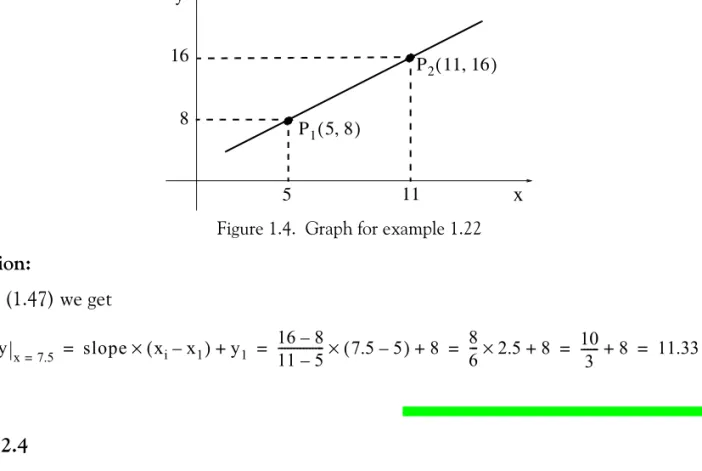
Given the graph of Figure 1.4, perform linear interpolation to compute the value of that corre-sponds to the value

2 3 7 x y 4 P₁(3 2, ) P₂(7 4, ) slope= m rise run --- 4 2– 7 3– --- 2 4 --- 0.5 = = = = x_i y_i y_i–y₁ x_i–x₁ --- = slope y_i = slope×(x_i–x₁)+y₁ = m x( _i–x₁) y+ 1 y_i x_i x_i x_i 1 slope ---×(y_i–y₁)+x₁ 1 m ----×(y_i–y₁)+x₁ = = x₁ = 0 x_i = x y_i = y y₁ = b y = mx b+ y x = 7.5

(36)

Chapter 1 Elementary Algebra

Figure 1.4. Graph for example 1.22 Solution:

Using (1.47) we get

Note 2.4

The smaller the interval, the better the approximation will be obtained by linear interpolation. Note 2.5

It is highly recommended that the data points are plotted so that we can assess how reasonable our approximation will be.

Note 2.6

We must exercise good judgement when we use linear interpolation since we may obtain unrealis-tic values. As as example, let us consider the following table where x represents the indicated numbers and y represents the square of x, that is, .

If we use linear interpolation to find the square of 5 with the data of the above table we will find that x y 1 1 ... ... 6 36 8 5 11 x y 16 P₁(5 8, ) P₂(11 16, ) y _x₌_7.5 slope×(x_i–x₁)+y₁ 16 8– 11 5– ---×(7.5 5– ) 8+ 8₆--- 2.5 8× + 10 3 --- 8+ 11.33 = = = = = y = x2 y_x₌₅ slope×(x_i–x₁)+y₁ 36 1– 6 1– ---×(5 1– ) 1+ 35 5 --- 4 1× + 29 = = = =

(37)

Infinite Sequences and Series

and obviously this is gross error since the square of is , not .

1.9 Infinite Sequences and Series

An infinite sequence is a function whose domain is the set of positive integers. For example, when is successively assigned the values , , ,..., the function defined as

yields the infinite sequence , , ,.... and so on. This sequence is referred to as infinite sequence to indicate that there is no last term. We can create a sequence by addition of numbers. Let us suppose that the numbers to be added are

We let

(1.49)

An expression such as (1.49) is referred to as an infinite series. There are many forms of infinite series with practical applications. In this text, we will discuss only the arithmetic series, geometric series, and harmonic series.

1.10 Arithmetic Series

An arithmetic series (or arithmetic progression) is a sequence of numbers such that each number dif-fers from the previous number by a constant amount, called the common difference.

If is the first term, is the nth term, d is the common difference, n is the number of terms, and is the sum of n terms, then

(1.50) (1.51) (1.52) The expression 5 25 29 x 1 2 3 f x( ) 1 1 x+ ---= 1 2⁄ 1 3⁄ 1 4⁄ s_n { } u₁, , , , ,u₂ u₃ … u_n … s₁ = u₁ s₂ = u₁+u₂ … s_n u₁+u₂+u₃+… u+ n uk k=1 n

∑

= = a₁ a_n s_n a_n = a₁+(n 1– )d s_n n 2 --- a( ₁+a_n) = s_n n 2 --- 2a[ ₁+(n 1– )d] =

(38)

Chapter 1 Elementary Algebra

(1.53) is known as the sum identity.

Example 1.23

Compute the sum of the integers from to Solution:

Using the sum identity, we get

1.11 Geometric Series

A geometric series (or geometric progression) is a sequence of numbers such that each number bears a constant ratio, called the common ratio, to the previous number.

If is the first term, is the term, is the common ratio, is the number of terms, and is the sum of terms, then

(1.54) and for ,

(1.55)

The first sum equation in (1.55) is derived as follows: The general form of a geometric series is

(1.56) The sum of the first n terms of (1.56) is

k k=1 n

∑

= 12---n n 1( + ) 1 100 k k=1 100

∑

= 12---100 100 1( + ) = 50 101× = 5050 a₁ a_n nth r n s_n n a_n = a₁rn 1– r 1≠ s_n a₁1 r n – 1 r– ---= a₁–ra_n 1 r– ---= ra_n–a₁ r 1– ---= a₁+a₁r a+ ₁r2+a₁r3+… a+ ₁rn 1– +…

(39)

Geometric Series

(1.57) Multiplying both sides of (1.57) by we obtain

(1.58) If we subtract (1.58) from (1.57) we will find that all terms on the right side cancel except the first and the last leaving

(1.59) Provided that , division of (1.59) by yields

(1.60) It is shown in advanced mathematics textbooks that if , the geometric series

converges (approaches a limit) to the sum

(1.61)

Example 1.24

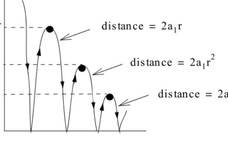
A ball is dropped from x feet above a flat surface. Each time the ball hits the ground after falling a distance h, it rebounds a distance rh where . Compute the total distance the ball travels. Solution:

The path and the distance the ball travels is shown on the sketch of Figure 1.5. The total distance

s is computed by the geometric series

(1.62) By analogy to equation of (1.61), the second and subsequent terms in (1.62) can be expressed as the sum of (1.63) s_n = a₁+a₁r a+ ₁r2+a₁r3+… a+ ₁rn 1– r rs_n = a₁r a+ ₁r2+a₁r3+… a+ ₁rn 1– +a₁rn 1 r– ( )sn a1 1 r n – ( ) = r 1≠ 1 r– s_n a₁1 r n

–

1 r–

---=

r <1 a₁+a₁r a+ ₁r2+a₁r3+… a+ ₁rn 1– +… s_n a1 1 r– ---= r 1< s = a₁+2a₁r 2a+ ₁r2+2a₁r3+… 2a₁r 1 r–

(40)

---Chapter 1 Elementary Algebra

Figure 1.5. Sketch for Example 1.24 Adding the first term of (1.62) with (1.63) we form the total distance as

(1.64) For example, if and , the total distance the ball travels is

1.12 Harmonic Series

A sequence of numbers whose reciprocals form an arithmetic series is called an harmonic series (or

harmonic progression). Thus

(1.65) where

(1.66) forms an harmonic series.

Harmonic series provide quick answers to some very practical applications such as the example that follows.

Example 1.25

Suppose that we have a list of temperature numbers on a particular day and time for years. Let a1 a1r3 a1r a1r2 distance = a₁ distance = 2a₁r distance = 2a₁r2 distance = 2a₁r3 s a₁ 2a1r 1 r– ---+ a₁1 r+ 1 r– ---= = a₁ = 6 ft r = 2 3⁄ a 6 1 2 3+ ⁄ 1 2 3– ⁄ ---× 30 ft = = 1 a₁ --- 1 a₁+d --- 1 a₁+2d --- _… 1 a₁+(n 1– )d --- _… , , , , , 1 a_n --- 1 a₁+(n 1– )d ---= 50

(41)

Proportions

us assume the numbers are random, that is, the temperature on a particular day and time of one year has no relation to the temperature on the same day and time of any subsequent year.

The first year was undoubtedly a record year. In the second year, the temperature could equally likely have been more than, or less than, the temperature of the first year. So there is a probability of that the second year was a record year. The expected number of record years in the first two years of record-keeping is therefore . For the third year. the probability is that the third observation is higher than the first two, so the expected number of record temperatures in three years is . Continuing this line of reasoning leads to the conclusion that the expected number of records in the list of observations is

For our example, and thus the sum of the first terms of harmonic series is or record years. Of course, this is the expected number of record temperatures, not the actual. The partial sums of this harmonic series are plotted on Figure 1.6.

Figure 1.6. Plot for Example 1.25

1.13 Proportions

A proportion is defined as two ratios being equal to each other. If

(1.67) where a, b, c, and d are non−zero values, then

(1.68) (1.69) 1 2⁄ 1 1 2+ ⁄ 1 3⁄ 1 1 2+ ⁄ +1 3⁄ n 1 1 2+ ⁄ +1 3⁄ +… 1 n+ ⁄ n = 50 50 4.499 5 1 1.000000 2 1.500000 3 1.833333 4 2.083333 5 2.283333 6 2.450000 7 2.592857 8 2.717857 9 2.828968 10 2.928968 11 3.019877 0 1 2 3 4 5 0 5 10 15 20 25 30 35 40 45 50 a b --- c d ---= a b+ b --- c d+ d ---= a b– b --- c d– d ---=