Occluded object tracking with RNNs

(1)

HAL Id: hal-02068351

https://hal.archives-ouvertes.fr/hal-02068351

Submitted on 14 Mar 2019

HAL is a multi-disciplinary open access

archive for the deposit and dissemination of

sci-entific research documents, whether they are

pub-lished or not. The documents may come from

teaching and research institutions in France or

abroad, or from public or private research centers.

L’archive ouverte pluridisciplinaire HAL, est

destinée au dépôt et à la diffusion de documents

scientifiques de niveau recherche, publiés ou non,

émanant des établissements d’enseignement et de

recherche français ou étrangers, des laboratoires

publics ou privés.

Occluded object tracking with RNNs

Mathis Petrovich

To cite this version:

Mathis Petrovich. Occluded object tracking with RNNs. [Research Report] Ecole normale supérieure

de Cachan; Carnegie Mellon University. 2018. �hal-02068351�

(2)

Occluded object tracking with RNNs

Mathis Petrovich

M1 student in Computer Science at the ´Ecole Normale Sup´erieure Paris-Saclay 2017-2018 Internship in the Robotic Institute at Carnegie Mellon University

Pittsburgh, PA 15217, the United States About 5 month (26 February 2018/20 July 2018)

Supervised by Martial Hebert

mathis.petrovich@ens-paris-saclay.fr

Abstract

Object detection in images has received a lot of attention in the recent years with state-of-the-art having human level performance. A lot of credit for such perfor-mance goes to the emergence of Deep Convolutional Neural Networks in partic-ular and Neural Networks in general. Extending the capabilities to videos is a fundamentally more challenging task. Recent approaches in the field have mostly used a frame-based detector and linked those detections across time. A major problem with all existing work is the incapability to handle occlusion, as in cases of occlusion the detector fails to output a result and hence so does the linker. Such scenarios of occlusion are very common in human-robot-interaction where the robot has to track objects which might get occluded by the human hand. In this internship, I worked with a team of researchers with the aim of creating a tracking system which is robust to partial as well as total occlusion.

(3)

1 Introduction

I worked with a team of three persons. Every week, we had a meeting with my advisor to show some progress and to have advice for the next things to do.

In Carnegie Mellon University, I had the opportunity to attend a lot of conferences and thesis propos-als. These presentations were very useful to open my mind to other approaches and other domains in computer science and robotics.

I would like to thank my advisor Martial Hebert for his time and all his advise, Lynnetta Miller for helping me with some administrative things and my team (Satyaki Chakraborty, Vivek Roy and David Russel).

2 Background requirement

2.1 What is a tracker?

A tracker is a system which takes as input a video and gives a list of tubelets as output. A tubelet is a list of bounding boxes where each bounding box belongs to one frame and all correspond to the same instance of object.

If there are two cats in a video, the output of the system will be two tubelets - the first one is the list of bounding boxes of cat1in every frame and the second one similarly for cat2.

We want to have a system that can track an object instance across time. 2.2 Neural Networks

What is a Neural Network?

An artificial neuron or perceptron is a concept in computer science which is a mathematical repre-sentation of a neuron in the human brain. We can think an artificial neuron as a function f : Rn→ R. An Artificial Neural Network (ANN), or simply a Neural Network (NN), is a collection of connected neurons working together to estimate more complex functions.

Why do we need Neural Networks?

High dimensional functions are fundamental constructs as such that we can think of any task as a function of inputs which returns the output. We can think of the task of Object Detection as a function from an input to the bounding box and class of an object. This idea of modelling tasks as functions helps us utilize the power of Neural Networks as Universal Function Estimators to solve the task at hand. The advantage of using NNs for solving problems is that the researcher/programmer does not have to meticulously design a function that maps input to output. NNs have the capability to learn a mapping from the input to the output. Given enough data (ordered pairs of input and output values) we can train a NN to learn the mapping with respectable levels of accuracy.

Components of a NN

A NN consists of neurons, connections and weights, a propagation function and finally a learning rule.

Neuron: A neuron with label j receiving an input pj(t) from predecessor neurons consists of the

following components:

• an activation aj(t), depending on a discrete time parameter

• possibly a threshold θj, which stays fixed unless changed by a learning function

• an activation function f that computes the new activation at a given time t + 1 from aj(t),

θjand the net input pj(t) giving rise to the relation aj(t + 1) = f (aj(t), pj(t), θj)

(5)

Often the output function is simply the Identity function.

An input neuron has no predecessor but serves as input interface for the whole network. Similarly an output neuron has no successor and thus serves as output interface of the whole network. Connections and weights: The network consists of connections, each connection transferring the output of a neuron i to the input of a neuron j. In this sense i is the predecessor of j and j the successor of i. Each connection is assigned a weight wij.

Propagation function: The propagation function computes the input pj(t) to the neuron j the

outputs oi(t)(t) of predecessor neurons and typically has the form:

pj(t) =Pioi(t)wij.

Learning rule: The learning rule is a rule or an algorithm which modifies the parameters of the neural network, in order for a given input to the network to produce a favored output. This learn-ing process typically amounts to modifylearn-ing the weights and thresholds of the variables within the network.

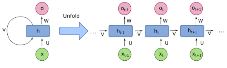
Recurrent Neural Networks (RNNs)

A Recurrent Neural Network is a type of Artificial Neural Network in which there is a recursive connection from the output to the input of the cell as shown in Figure 1. We can think of it as a feedback mechanism in which the network accounts for the output it produces at a previous point in time.

Figure 1: A recurrent connection can be unfolded in time. This helps us visualise how the input is propagated forward in time.

RNNs are used to have a form of memory. Since the cells account for the output generated by it at a previous point in time, it can make its predictions keeping its past predictions in mind. As such a RNN learns what predictions are/can be important at a later point in time and remembers them, while forgetting the rest. This kind of memory is important in certain uses of NNs and hence RNNs have been used profoundly in tasks of Natural Language Processing (NLP) and Digital Signal Processing (DSP).

LSTM networks: Long Short Term Memory (LSTM) networks is a kind of recurrent network which has some kind of memory cells and has the ability to keep some information and discard others.

2.3 Intersection Over Union (IoU) metric Introduction

Having a good metric is something crutial in machine learning and computer vision. It is useful to compare results and it is very important in the learning process (to compute the loss function). For image detection the most common one is IoU (Intersection over Union) (see the Figure 2 to look at the definition)

(6)

Figure 2: Computation of the IoU

How to use it

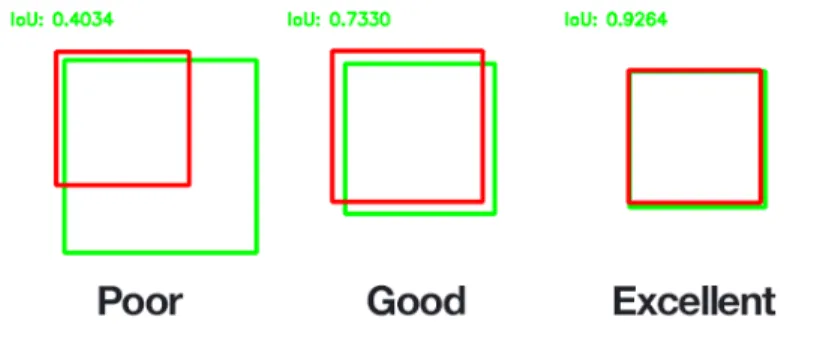
Two bounded areas are required in order to compute IoU. In our case, we use the ground truth (the real coordinate of the bounding box) and the bounding box output of our algorithm. (Figure 3 shows what a result could be like.

Figure 3: Example of IoU

Some can define a threshold (often th = 0.5) and say that a detection is valid if and only if IoU ≥ th. In this report, I will call mIoU the average of the IoU according to a dataset and mdetection the average of valid detection (1 for valid and 0 otherwise).

3 What is the goal of my internship

We want to create a tracker which can robustly track objects even when it is experiencing partial, total occlusion or fast motion.

3.1 What is the occlusion we want to catch

Our goal is to continue the tracking even when there are occlusions.

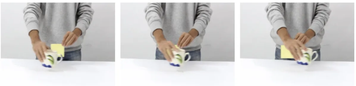
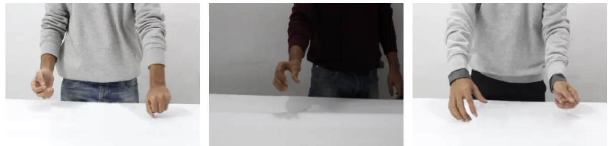
There is different type of occlusions, there is the more common one: the dynamic occlusion (Figure 4). There is also static occlusion (like Figure 5).

And also, there is the difficulty when the detector doesn’t detect an object because of orientation (Figure 6) or fast movement (Figure 7)

3.2 Different type of tracker There is two different kinds of trackers:

(7)

Figure 4: Dynamic occlusion

Figure 5: Static occlusion

Standard tracking

Use only the content of the frame, no detector needed. This method has the advantage to be very fast (up to 100 fps [10]), and can track anything (even not a known object, like a background). I did some experiments with this technique in the Section 6.

Tracking by detection

This method uses an object detector, and tries to use this extra information to track objects. It is used by the state of the art, and works better than normal tracking (but slower).

In this research, there is no constraint about speed. This is why we used this method.

4 Datasets

I have worked on two kinds of datasets. • A new one, which I will call custom • A standard one: ImageNetVid

(8)

Figure 7: Fast movement

4.1 The custom dataset

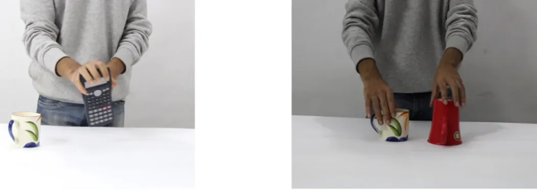
To be able to handle occlusions, and to test our system on this point, we need a dataset to train our system and to test it to have qualitative results. Unfortunately, there is no annotated dataset with occlusions. My team created a dataset with 300 videos (5h of videos) to be able to do that. (see Figure 8) These videos are indoor and use 12 different objects (mug₁, mug₂, ball, stapler etc).

(a) calc and mug1 (b) mug1and mug2

Figure 8: Some visualisation of this dataset

Features

This is an instance based dataset, so there is no more than one same object in the scene (this is why mug₁6= mug₂) (Figure 9)

(a) Objects based (b) Instance based

(9)

Annotations

Because it is a new dataset, annotations are not present (we don’t know where are the objects). So we needed to annotate it. With a tool, I helped them to annotate about 100 videos. This was long but it is a very important step. At each frame, I needed to draw a bounding box and give the name of the object. Thanks to interpolation, it was quicker than I expected.

Object detector

To be able to train and test our system with this dataset, a object detector is needed. Because of the nature of objects (different instance of mug, stapler etc), there is no out of the box object detector. For the training of this detector, we don’t want to use real frames of this dataset because we want to keep them just for the training of the system. Here comes the idea of generating synthetic data. According to the the paper [12], I took samples of backgrounds (Figure 11) to create a new dataset of about 50000 images (exemple Figure 12)

Our team chose Faster R-CNN [7] because it is good deep learning based detector, it is recent and fast. It uses a CNN (Convolution Neural Network) in order to have feature maps. With them, a Region Proposal Network is used to give rectangular object proposals with a objectness score (see Figure 10). Then a classifier is used to choose the class of a particular bounding box.

Figure 10: Schema of Faster RCNN

In order to use it, I took a pre-trained version of it (trained with the large dataset ImagenetDet [8]). Then, I used the synthetic dataset (see Figure 11) to finetune the detector on our objects. Finally, I computed all the detections of the entire dataset. I did that to be able to use and reuse detection during the training of our system and during testing without recomputing everything at each step. Splitting the data

Like every dataset, we need to split it in 3 parts. The first one is the training part, we tell our system the right output and train our system to get it (around 80%). The second one is the validation part, this one is here to be able to not do over-fitting on the training dataset (learning without generaliza-tion). For each step of the training (epoch), we evaluate our system on the validation. If the loss of the validation is not decreasing, we need to stop the training (even if the loss of the training part

(10)

Figure 11: Some backgrounds without object used for generating synthetic data

Figure 12: Some synthetic data to train an object detector for the custom dataset

continues to decrease). The third one is the test dataset. We need it to test our system (we will not use it at all during training).

4.2 ImageNetVid dataset

This dataset is important to be able to have comparable result to the actual state of the art [13] (11 Oct 2017).

Features

This dataset is composed of 3 datasets (train ≈ 3000 videos, validation ≈ 500 videos and test ≈ 1000 videos)

It is a multi-objects based dataset: that means in one frame, it could have more than one turtles for example (see example of this dataset Figure 13). Unlike our custom dataset, after doing the detection of an object, we need to match this object to the oldest one. (see the matching subsection)

(a) A turtle (b) A lizard

(11)

Object detector

To have a fair comparison, it is better to have the same detector as the state of the art. They use R-FCN ([9], a variant of Faster-RCNN [7], a region based detector).

This detector predicts first region proposal (bounding boxes without label) and after it uses a clas-sifier to identify each box with each object (taking the one with the highest confident score). We extracted the detector from their code, and computed the detections on the whole dataset.

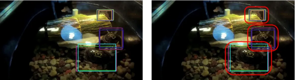
The problem is that there are too much boxes in the output. If we just take a threshold (0.9 for example), this will remove a lot of false positives but for a single object, a lot of boxes can still be there (see Figure 14).

(a) Multiple detection for one object (b) Clustering of bounding boxes

Figure 14: Pre-output of the detector of ImageNetVid To avoid this behaviour, we need to do some kind of clustering. (see Figure 14)

There are several ways to do that. The first way I though was to apply the Mean Shift algorithm [2] because it works very well in general. One of the drawback of this algorithm is its slowness. After looking at some other research papers (like [13] for example), we decided to go with Non Max Suppression (NMS).

Non max suppression:

• Sorting all the boxes by decreasing score

• For each box, remove all the remaining boxes if the IoU > th With the process, the result of this detector is way cleaner.

5 Optical flow

5.1 Introduction

To be able to handle occlusions, our model needs some kind of notion of movement. We chose to use optical flow because it tries to capture the displacement of each pixel in an image.

By definition, the optical flow between two frames is the apparent motion of pixels of one frame to the other.

There are two kinds of optical flows:

• Discrete optical flow: a grid of vectors

• Dense optical flow: compute ∆xand ∆yfor each pixel

Dense optical flow makes more sense in our system because the goal of the optical flow is to be fed into a neural network.

(12)

5.2 Choose of the algorithm

There are a lot of different ways to compute it.

First I tried the state of the art Flownet2 [11]. It is a deep learning based approach, data are fed into a lot of sub-networks. The results were excellent but the problem is that it was very long to compute (about 4 seconds per frame, more than 1 hour per video).

The second option, used by a lot of people, is to use the Farneback optical flow [3]. It is a very fast algorithm (about 5 min for one video) and the results are fine.

Finally, according to some recent articles, we decided to try the Brox optical flow [4]. Surprisingly, it is as fast as Farneback (5 min for each video, because it is implemented with GPUs) but the result are more consistent.

(a) Flownet2 (b) Farneback (c) Brox

Figure 15: This is the visualisation of the optical flow for the video 0000.mp4 of the custom dataset. Each color is mapped with a direction. For example black is no movement, red is displacement to the right and blue to the left.

5.3 Storage

In machine learning, a lot of data have to be processed. In CMU remote server, optical flow can’t be saved directly because it will take too much space. I had to find a solution to keep ”good” optical flow but without having too large files.

The first approach I tested was the simplest one: saving the type of data to float32 to float16. Un-fortunately this was not enough. Flows are still very heavy. To improve this approach, I resized the optical flow to a fixed size (512x512). This reduced the size again but several problems appeared.

• Resizing does not depend on the size of the video (very sparse in ImageNetVid) • Loss of quality during resizing (interpolation etc)

• Still large files

To be able to be more effective, I took the idea of [5] and implemented efficiently: 1. Saving mx= min(∆x), Mx= max(∆x) and my= min(∆y), My= max(∆y)

2. Mapping the input to [0, 255] • Applying fx→

(fx−mx)∗255

(Mx−mx) for every ∆x

• Applying fy →(f_(My−my)∗255

y−my) for every ∆y

3. Changing the type to uint8 and save as 2 JPEG greyscale images for x and for y

For the custom dataset, this process decreases the size from 1.5 TB to 21 GB (more than 70x less). The quality of the flow is still good enough.

(13)

6 Study of the Goturn tracker

6.1 Introduction

To have some experience with tracking, to have some comparable results and also to learn machine learning framework, I worked on the paper [10].

This is a very simple method, it works very well and it is very fast. 6.2 How it works

After training (on images and videos), you just have to feed a cropped image with the actual bound-ing box into the network and it will output the next boundbound-ing box.

This is very fast but it can fail when there is overlapping of several objects (occlusions 4). Because this model doesn’t have a notion of the object it is tracking, in one ambuiguous frame, it can choose another object and continue to track the wrong one for the rest of the video.

6.3 Some results on the custom dataset

Fine-tuning: This is when we take a pretrained network to retrain it on another dataset with a smaller learning rate (to avoid overfitting)

To be able to see results, I fine-tuned this network with a train dataset and tested on a test dataset. That is some results:

mIoU mdetection No fine-tuning 0.28 0.28 Fine-tuning 0.49 0.63

This tracker works pretty well after fine-tuning. Maybe a future work can be to try to merge this idea and the idea of the Section 7.

7 Our system

7.1 Architecture of our system

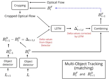
To be able to handle occlusions, our system needs to try to understand a motion model. This is why we are using optical flow and a LSTM network.

Our approach used informations from the previous frame to estimate the position in the actual frame. The optical flow information helps the network to have an idea of motion of the object. Then, the LSTM network will try to understand the motion (of the optical flow) and use the bounding box for the detector (or the current one if there is none) to predict the next bounding box.

This system works as a tubelet corrector. To be precise, this is the first idea: 1. Cropping the optical according to the last bounding box

2. Extracting features with a CNN

(14)

4. Collecting the output: bounding box of the next track 5. Combining this box with the detection

The fact of feeding the bounding box in the LSTM can cause a lot biases during the training (we don’t have enough data to be position invariant). So instead of that, we decided to take the delta between the detection and the last corrected output (see a schema Figure 16)

Figure 16: Schema of the architechture of the network

Modularity: This architecture is modular so we can plug and play other object detector and other optical flow (according to the time we have to compute them). The idea behind such modularity is to be able to well train the LSTM network and use that in a new environment with other ob-jects/backgrounds (and so a new object detector) without retraining everything.

7.2 Training

Training a recurrent network is something hard to do because The output of the system is used as input to the next iteration. Such a system is trained by taking a set of consecutive ground truth output.

We are using the smooth L1 function for training (defined in [6]) because it is less sensitive to

outliers and gradient explosion (compared to regular L2)

Teacher forcing

There are different ways to learn a recurrent neural network. For LSTM, teacher forcing is a way of learning which has a lot of advantages.

Teacher forcing works by using the actual or expected output from the training dataset at the current time step y(t) as input in the next time step X(t+1), rather than the output generated by the network. 7.3 Optical flows features

Instead of feeding the raw optical flow into the system, it is first given to a CNN network (neural network with Convolutionnal layers) to extract features. The system will learn to extract the good features to obtain wanted output.

7.4 Combining

In this architecture, we let at the end the possibility to combine the output of the system with the output of the detector (if there is one). This can reduce the possibility of our system to drift and/or

(15)

change object (if there is a long occlusion). We did some experiment with some values (1 and 0) or (1 − α and α).

7.5 Limitation of this approach

For now, we don’t take care of false positives (if there is a bad detection with high confidence score we can try to track anything, so we took the assumption that the detector is quite good). Also, we can give birth to a track (if an object appears) but we didn’t think yet about how to kill a track (when an object leaves the scene etc). Also, our architechture didn’t produce a confidence score. So, we can’t yet really compare the results with the same metric than Detect to Track and track to detect [13] (because the mAP metric uses confidence score).

7.6 Results

On the custom dataset, we just did some qualitative experiments. It works in a lot of cases when the detector is working. However there are still problems when we try to track objects with bad detections (for example with the ball or the stapler). For some reasons, this system creates a small drift every frame. To fix that, we just did some kind of threasholding with rounding.

To see some results, I computed the tracks and see the difference between [only detection and match-ing] and [detection correction and matchmatch-ing] (for the imageNetVid dataset).

only matching only tracking combine both

mIoU 0.48 0.42 0.62

We can see that our system works better when we combine the output of the LTSM with the output of the detector. This also shows that the system works better than without it (only matching). 7.7 Multi-object tracking: matching

In each step, the detections have to be matched with the current track because it is possible to have multiple instances of a object in a frame. This can be done in a lot of different way. To avoid spending too much time on this problem, we decided to take a common approach: applying the hungerian algorithm [1] on the two sets of boxes with the distance:

d(boxA, boxB) = 1 − IoU (boxA, boxB)

This worked well in a lot of cases but can fail when there are two objects which are close and/or when there are occlusions with two instances of the same object. (It is ”frame based”, there is no idea of motion in the matching process). To improve that, it should be interesting to change the distance and incorporate the idea of localisation and velocity.

8 Technical details

In this project, we are using Python2 with Tensorflow. I worked remotely in ssh into the server. I was able to use 4 Nvidia GeForce GTX 1081 Ti and a 32 cores CPU with 126 GB of RAM. Thanks to that, we were able to some improvement in the training process.

8.1 Multi GPU training

In Tensorflow, doing multi GPU training is not an easy task and there are a lot of ways to do it. We chose the one which is the more natural for us:

1. Copying the model on each GPUs 2. Giving different batches on each GPUs 3. Computing gradients individually 4. Averaging gradients in the CPU 5. Updating weights on each GPUs

(16)

9 Conclusion

This internship helped me to learn a lot of machine learning and computer vision theory. I now understand how state-of-the-art works in some computer vision tasks. I improved my skills in Python and machine learning framework.

In this project, I worked on a new dataset where I was able to experiement a lot. I saw some important steps in the creation of a new dataset.

I read a lot of recent articles which give me a lot of knowledge in computer vision and machine learning. I did experiments with some articles. This gave me some idea of the way trackers works. Then we tought the way to improve the actual tracker in order to be better on occlusions cases. After designing the architechture of the system (with recurrent network), I did experiments to see if it works. For the general case, it works less good than other approach (but it is not too bad). To be able to have comparable results with the state-of-the-art, it is needed to change the way our system works (because of the way evaluation works)

I worked with a lot of people of different countries. This was a very interesing internship.

References

[1] H. W. Kuhn and Bryn Yaw. “The Hungarian method for the assignment problem”. In: Naval Res. Logist. Quart(1955), pp. 83–97.

[2] Dorin Comaniciu and Peter Meer. “Mean Shift: A Robust Approach Toward Feature Space Analysis”. In: IEEE Trans. Pattern Anal. Mach. Intell. 24.5 (May 2002), pp. 603–619.ISSN: 0162-8828.DOI: 10.1109/34.1000236.URL: http://dx.doi.org/10.1109/ 34.1000236.

[3] Gunnar Farneback. Two-Frame Motion Estimation Based on Polynomial Expansion. June 2003.

[4] Thomas Brox et al. “High Accuracy Optical Flow Estimation Based on a Theory for Warp-ing”. In: ECCV. 2004.

[5] Karen Simonyan and Andrew Zisserman. “Two-Stream Convolutional Networks for Action Recognition in Videos”. In: CoRR abs/1406.2199 (2014). arXiv: 1406.2199.URL: http: //arxiv.org/abs/1406.2199.

[6] Ross B. Girshick. “Fast R-CNN”. In: CoRR abs/1504.08083 (2015). arXiv: 1504.08083.

URL: http://arxiv.org/abs/1504.08083.

[7] Shaoqing Ren et al. “Faster R-CNN: Towards Real-time Object Detection with Region Pro-posal Networks”. In: Proceedings of the 28th International Conference on Neural Informa-tion Processing Systems - Volume 1. NIPS’15. Montreal, Canada: MIT Press, 2015, pp. 91– 99.URL: http://dl.acm.org/citation.cfm?id=2969239.2969250.

[8] Olga Russakovsky et al. “ImageNet Large Scale Visual Recognition Challenge”. In: Inter-national Journal of Computer Vision (IJCV)115.3 (2015), pp. 211–252.DOI: 10.1007/ s11263-015-0816-y.

[9] Jifeng Dai et al. “R-FCN: Object Detection via Region-based Fully Convolutional Networks”. In: Advances in Neural Information Processing Systems 29. Ed. by D. D. Lee et al. Curran Associates, Inc., 2016, pp. 379–387.URL: http://papers.nips.cc/paper/6465-r- fcn- object- detection- via- region- based- fully- convolutional-networks.pdf.

[10] David Held, Sebastian Thrun, and Silvio Savarese. “Learning to Track at 100 FPS with Deep Regression Networks”. In: European Conference Computer Vision (ECCV). 2016.

[11] Eddy Ilg et al. “FlowNet 2.0: Evolution of Optical Flow Estimation with Deep Networks”. In: CoRRabs/1612.01925 (2016). arXiv: 1612.01925.URL: http://arxiv.org/abs/ 1612.01925.

[12] Debidatta Dwibedi, Ishan Misra, and Martial Hebert. “Cut, Paste and Learn: Surprisingly Easy Synthesis for Instance Detection”. In: The IEEE International Conference on Computer Vision (ICCV). Oct. 2017.

(17)

[13] Christoph Feichtenhofer, Axel Pinz, and Andrew Zisserman. “Detect to Track and Track to Detect”. In: CoRR abs/1710.03958 (2017). arXiv: 1710.03958.URL: http://arxiv. org/abs/1710.03958.