How and to what extent support to agriculture affect farmland markets and prices: a literature review

HAL Id: hal-02813823

https://hal.inrae.fr/hal-02813823

Submitted on 6 Jun 2020

HAL is a multi-disciplinary open access archive for the deposit and dissemination of sci-entific research documents, whether they are pub-lished or not. The documents may come from teaching and research institutions in France or

L’archive ouverte pluridisciplinaire HAL, est destinée au dépôt et à la diffusion de documents scientifiques de niveau recherche, publiés ou non, émanant des établissements d’enseignement et de recherche français ou étrangers, des laboratoires

How and to what extent support to agriculture affect

farmland markets and prices: a literature review

Laure Latruffe, Chantal Le Mouël

To cite this version:

Laure Latruffe, Chantal Le Mouël. How and to what extent support to agriculture affect farmland markets and prices: a literature review. JADE#34145, 2006. �hal-02813823�

JADE#34145

How and to what extent support to agriculture affect farmland markets and prices: A literature review

Laure Latruffe and Chantal Le Mouël

INRA-ESR, 4 allée A. Bobierre, CS 61 103, 35 011 Rennes cedex, France1*

Report for the OECD, Directorate for Food, Agriculture and Fisheries

27 March 2006

1

Laure.Latruffe@rennes.inra.fr ; Chantal.LeMouel@rennes.inra.fr

1. Introduction ... 4

2. Agricultural support does affect farmland markets and prices: Insights from the theory ... 4

2.1. Farmers’ production decisions, agricultural support and the rental price of land ... 5

2.1.1. Output price support and farmland rental markets and prices... 5

The one output-one factor case: Illustrating the key role of factor supply elasticity... 6

The one output-two factor case: Illustrating the key role of factor substitution possibilities.... 11

2.1.2. Factor subsidies and farmland rental markets and prices ... 15

The one output-one factor case: Illustrating the key role of factor supply elasticity... 15

The one output-two factor case: Illustrating the key role of factor substitution possibilities.... 19

2.1.3. factor supply price elasticities and substitution elasticities: Discussion ... 25

Factor supply elasticities: Indicators of the extent of mobility of factors ... 25

Elasticities of substitution: Indicators of the flexibility of the technology... 28

2.1.4. Some modelling issues ... 29

Global simulation models deal only with farmland rental markets and rely on uncertain parameter values... 30

Representation of agricultural support policy instruments and programmes: The main drawback of global simulation models... 31

2.2. Farmers’ production intertemporal decisions, agricultural support and the sale price of land... 38

2.2.1. The relationship between farmland rental price, farmland value and farmland sale price: The present value framework ... 38

The basic capitalisation formula... 38

Various refinements of the basic capitalisation formula ... 39

2.2.2. The present value approach questioned... 42

3. Agricultural support does affect farmland markets and prices: Empirical evidence... 44

3.1. Methods used in the empirical studies: evolution of the present value model and other approaches ... 44

Specification of varying or different discount rates ... 45

Treatment of expectations ... 46

Account for alternative land uses ... 47

Other extension... 47

3.1.3. Other methods used ... 47

3.2. Findings from the empirical studies: Extent of the impact of agricultural policy ... 48

3.2.1. Evidence of the effect of public support on land prices ... 48

3.2.2. Estimation of the elasticity of the land values with respect to the support... 49

Elasticity of land prices with respect to the support... 49

Elasticity of land rentals with respect to the support... 51

Dilution and uncertainty ... 52

3.2.3. Evaluation of the share of land value accounted for by support; effect of removal of support ... 53

3.2.4. Who benefits from the capitalisation? ... 55

1. Introduction

A central purpose of agricultural policies in OECD countries is to support farmers’ income. Whether agricultural support actually benefits farmers however is an open question. Agricultural support policies raise farmers’ gross income and then contribute to increase returns to resources that individual farmers use. As a consequence agricultural support policies contribute to increase the market prices of these resources and ultimately benefit the owners of these resources. Hence, whether agricultural support benefits farmers closely depends on whether farmers own the resources they use in production.

Among agricultural primary factors of production (land, family labour and capital), land has been paid higher attention regarding this issue for at least two reasons. First of all in a lot of OECD countries, a substantial share of farmland is rented, sometimes from other farmers but also commonly from non-farmer landlords. Secondly in all OECD countries an increasing number of government payments are tied to farmland. Hence the question of the extent to which agricultural subsidies do translate into higher land values and rents and finally benefit landowners is a critical issue.

Concern over the capture of agricultural policy benefits by the landowners is not new. And the question of the capitalisation of support into farmland values and rents has a long tradition in Agricultural Economics. The objective of this report is to provide an overview of existing literature on that subject.

This overview is organised along two lines. The first section reviews the main insights that can be drawn from the theory about how agricultural support may affect farmland values and rents and what are the key assumptions and parameters regarding this issue. The second section reviews empirical evidence about the extent to which agricultural support affects farmland values and rents.

2. Agricultural support does affect farmland markets and prices: Insights from the theory By which mechanisms agricultural support does affect farmland markets and prices? What are the main assumptions and parameters that play a key role as regards the extent of the impact of agricultural support on farmland markets and prices? Who finally benefit from agricultural support? This section synthesises the main insights that can be drawn from the theory regarding these 3 questions. The relationships between agricultural support and farmland rental markets and prices (i.e., when farmland is considered as a production factor) are investigated first. Then, we focus on the relationships between agricultural support and farmland sale markets and prices (i.e., when farmland is considered as an asset).

very simple analytical frameworks that are designed to illustrate these mechanisms. This first step allows to detect the key assumptions and parameters regarding the extent of the impact of agricultural support on farmland markets and prices. Then these key assumptions and parameters are discussed. Finally, implications on the relevance of aggregate models (such as the PEM model developed by the OECD) for assessing the impact of various agricultural policy reforms are derived.

Examining the impact of all kinds of policy instruments on farmland markets and prices would be too long and out of the scope of this study. Hence we concentrate on two types of policy instruments: output price support and land subsidy. These both instruments have been selected because they reflect the evolution of agricultural policies in OECD countries over the last decade where output price support has been progressively replaced by direct payments linked to production factors, especially land.

2.1. Farmers’ production decisions, agricultural support and the rental price of land

The main insights that can be drawn from theory on the effects of output price support on farmland rental markets and prices are first reviewed. Then, we focus on what we do know from the theory about the effects of factor (especially land) subsidies.

In both cases, using very simple frameworks, the main mechanisms that underlie the effects of policy instruments are described by the mean of a graphical analysis, while corresponding analytical results are reported in appendix. This first step allows to point out the key assumptions and parameters as regards the extent of the effects of policy instruments on farmland markets and prices.

Then, the sub-section follows with a discussion on these assumptions and parameters and ends with some modelling issue considerations.

2.1.1. Output price support and farmland rental markets and prices

One paper extensively cited in the existing literature is Floyd (1965). This seminal paper shows, using a rather simple analytical model, that: i) output price support affects the prices of production factors2; ii) the extent of the impact of output price support on factor prices closely depends on the elasticities of supply of factors (that is the extent of factor mobility within the economy) and on agricultural production technology (that is, specifically, the extent of factor substitution possibilities); iii) output control programmes (through production quota or acreage restriction) modify the effect of output price support on factor prices either by creating a new fixed production factor (production rights) in the case of the quota or by changing the opportunity cost of land in the case of acreage restriction.

2

In this report the term production factors refer to land, family labour and capital while the term inputs designate all other (variable) inputs such as hired labour, energy, fertiliser, pesticides, etc.

A number of papers have re-examined in alternative ways Floyd’s results or extended them by relaxing restrictive hypotheses of Floyd’s model and/or including various alternative policy instruments in order to compare their respective effects (e.g., Gardner, 1987; Hertel, 1989; 1991; Leathers, 1992; Dewbre et al., 2001; Dewbre and Short, 2002; OECD, 2002a; Guyomard et al., 2004). Usually however, although analytical results are much more complicated and effects of policy instruments more difficult to disentangle, interpret and sign, main insights from Floyd’s model do remain.

The one output-one factor case: Illustrating the key role of factor supply elasticity

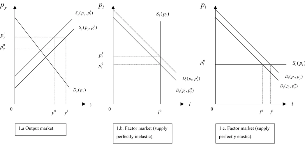
Let’s consider a representative farmer using one factor (which may be land) in quantity l to produce an aggregate agricultural output in quantity y, according to a given production technology (y= f(l)). Figure 1 below depicts the domestic output and factor markets in the considered country. On the output market, D_y(p_y) is the domestic demand while

S

_y

(

p

_y

,

p

_l0

)

is the initial domestic supply. Both the domestic demand and supply depend on the domestic output price p_y. The initial output supply also depends on the initial equilibrium price of the factor p_l0. Let’s assume that the considered country is a small country for the output y. Hence, at initial equilibrium domestic output price is

p

0_y corresponding to the exogenous world price. The representative farmer produces quantity

0

y , which is partly consumed domestically and partly exported. On the factor market,

D

_l

(

p

_l

,

p

0_y

)

is the initial domestic derived demand, as a function of the factor price and the initial output price, while

) ( _l l p

S is the domestic factor supply. On panel 1.b this factor supply is assumed to be perfectly inelastic in quantity l0 (l is a specific factor to agriculture), while in panel 1.c it is assumed as perfectly elastic at price p_l0. Let’s assume that the factor is not traded. Hence, in both cases, at initial equilibrium domestic demand equals domestic supply at price p_l0 and quantity l0.

Let’s imagine that the government decides to support the farmer’s income through output price support. Hence the output price increases to

p

1_y.3 In a first step, this output price increase is an incentive for the farmer to produce more. Other things being equal, the farmer would seek to produce

3

This output price support may be provided through a fixed support price or a fixed (ad-valorem or specific) output subsidy. Such alternative instruments would have different impacts for domestic consumers and in terms of net welfare loss for the considered country but not for the representative farmer, nor on the factor market. As we are only interested in the farmer’s situation in conjunction with the impact of output price support on the

1

y . However, such an output supply increase would require to use more factor. This factor adjustment requirement is depicted through the shift in the derived curve from

(

,

0

)

y l l

p

p

D

to

(

,

1

)

y l l

p

p

D

on the

factor market. At this stage one guesses the key role of the factor supply elasticity:

- In panel 1.b, as the factor supply is perfectly inelastic (i.e., there is no additional quantity of factor available), this factor demand increase translates into a factor price increase from p_l0 to

1 l

p . This factor price increase makes the output more costly to produce. The resulting increase in the marginal cost of y is depicted on panel 1.a through the shift of the output supply curve from

S

_y

(

p

_y

,

p

_l0

)

to

S

_y

(

p

_y

,

p

1_l

)

. Finally, figure 1 shows that following the induced price adjustment on the factor market, the final equilibrium output quantity is unchanged in y0. - In panel 1.c, as the factor supply is perfectly elastic (i.e., at price p_l0 there is no restriction on

available quantity of the factor), the factor demand increase does not affect the factor price, which remains at p_l0 level. Hence, marginal cost of y is unchanged. Factor demand and output supply increase simultaneously, to y1 and l1 respectively.

Finally, figure 1 shows that the effects of output price support on both the output and the factor markets are quite different according to the level of the factor supply elasticity. One may synthesised the main findings as follows.

When the factor supply elasticity is low (the extreme case being zero, as illustrated by panel 1.b): - The increase in the price of the output is totally translated into an increase in the price of the

factor (as shown in appendix, the percentage change in the factor price equals the percentage change in the output price).

- As the factor becomes more expensive, price support indirectly increases the production cost of the output.

- The farmer’s surplus is unchanged since the totality of support provided through the output price is transferred to the owner of the factor.

- If the owner of the factor is the farmer, then the price support policy actually contributes to supporting the farmer’s income. At reverse, if the owner of the factor is not the farmer, but an individual who is outside the agricultural sector, the price support policy completely misses its initial objective since the provided support “leaves” the agricultural sector.

- On an intergenerational basis, by contributing to increase the price of the factor, the price support policy increases the cost of setting-up for future farmers. Finally, not only the price

support policy misses its initial target group (the current farmers) but also contributes to worsen the situation of future farmers.

When the factor supply elasticity is high (the extreme case being the infinity, as illustrated by panel 1.c):

- The increase in the price of the output translates into a quantity adjustment on the factor market and has no impact on the price of the factor.

- In that case, the production cost of the output is unchanged. Price support induces an increase in output supply.

- The farmer’s surplus increases since the totality of support provided through the output price is gained by the farmer. In that case, the price support policy actually contributes to supporting the farmer’s income.

- On an intergenerational basis, as the price support policy does not affect the factor price, it does not change the situation for future farmers.

Finally, if we consider that the factor in figure 1 is land, this figure illustrates the key role of the land supply price elasticity as regards the effect of output price support on the rental price of land: if this elasticity is very low, output price support is nearly totally “capitalised” in the rental price of land, while if this elasticity is very high, output price support has nearly no effect on the rental price of land. In other words, the lower the land supply price elasticity the higher the share of output price support “capitalised” in the rental price of land.

At this stage two remarks are in order. Firstly, it is commonly recognised that agricultural land supply elasticity is rather low (cf. discussion in point 2.1.3). Hence, in most OECD countries land supply is probably closer to the situation depicted in panel 1.b than in panel 1.c. In other words, it is most likely that in OECD countries the support (still or previously) provided to farmers through price support is or has been at least partially transferred to landowners and has finally, at least partially, not benefited to farmers who do not own their land.4 Secondly, most policy analyses that adopt a partial equilibrium framework implicitly assume that factor prices are exogenous and constant. In other words they implicitly adopt the framework of panel 1.c. This is obviously a restrictive assumption, especially regarding land. Therefore, one must keep in mind that all commonly admitted results in terms of market and welfare effects of alternative agricultural policy instruments are obtained conditionally on the constant factor price hypothesis. Panel 1.b clearly shows that once this hypothesis is relaxed, such

4

We acknowledge that the reality is far more complex than the situation described in figure 1 and that a great number of other factors do affect land rental price adjustment and the adjustment on agricultural output markets

effects may change. As an extreme illustration, in panel 1.b., one may consider that the price support policy is decoupled since following the factor price adjustment, it has no effect on the output supply quantity.

Figure 1. Effects of output price support on domestic output and factor markets: the one-factor case 1.a Output market 1.b. Factor market (supply

perfectly inelastic) y

p

p

_l

p

_l y l l 0 y y 0 y

p

0 l p 0 l p 0 l l0 1 y

p

1 y y 1 l p 1 l ) , ( y 0l y p p S ) , ( 1 l y y p p S ) ( _y y p D ( , ) 0 y l l p p D ) , ( l 0y l p p D ) , ( 1 y l l p p D ( , ) 1 y l l p p D 0 0 0 ) ( _l l p S ) ( _l l p S

1.c. Factor market (supply perfectly elastic)

The one output-two factor case: Illustrating the key role of factor substitution possibilities Let’s assume now that our representative farmer produces an aggregate agricultural output by combining two factors, according to a given production technology (y= f( xl, )). The first factor is land and is used in quantity l. The second factor may be an aggregate of family labour and capital and is used in quantity

x

. Figure 2 below depicts the domestic output and factor markets in the considered country.

Notations are similar to the previous case. Panel 2.b. describes the domestic land rental market. We assume that the land supply is imperfectly elastic and consequently increasing in the rental price of land. Panel 2.c depicts the domestic market of the other factor. The domestic supply of this other factor is assumed to be perfectly elastic in p_x0. On panel 2.a output supply now depends on the output price and on both factor prices. On panels 2.b and 2.c derived demands of factors also depend on the output price and on both factor prices. Therefore,

S

_y

(

p

_y

,

p

_l0

,

p

0_x

)

is the initial output supply curve, while

(

,

0

,

0

)

x y l l

p

p

p

D

and

(

,

0

,

0

)

l y x x

p

p

p

D

are the initial derived demand curves of land and of the other factor respectively.

All other assumptions adopted in the previous case are still valid here. At initial equilibrium the domestic output price is

p

0_y, the representative farmer produces quantity y0 using quantity l0 of land and quantity x0 of the other factor. The initial rental price of land is p_l0, while the initial price of the other factor is p0_x.

As in the previous case, we assume that, following the implementation of an output price support policy, the output price increases to

p

1_y. In a first step, this output price increase is an incentive for the farmer to produce more. Other things being equal, the farmer would seek to produce y1. However, such an output supply increase would require to use larger quantities of factors. This is at this stage that the key role of substitution possibilities between both factors does appear.

- Let’s consider first the case where both factors are highly substitutable. As the supply of factor

x

is perfectly elastic, an increase in its derived demand would have no impact on its initial equilibrium price. While as the supply of land is imperfectly elastic an increase in its derived demand would lead the land rental price to increase relative to its initial equilibrium level. Therefore, in the new output price context, the representative farmer who wants to increase his/her output quantity has incentive to change his/her factor quantity ratio in favour of factor

x

, trying to keep nearly unchanged his/her use of land. Such a situation is represented in panels 2.b and 2.c by the small shift to the right (from

(

,

0

,

0

)

x y l l

p

p

p

D

to

(

,

1

,

0

)

x y l sub l

p

p

p

D

)

of the derived demand of land and the large shift to the right (from

D

_x

(

p

_x

,

p

0_y

,

p

_l0

)

to

)

,

,

(

1 1sub l y x sub x

p

p

p

D

) of the derived demand of factor

x

. Hence, at final equilibrium, the farmer produces quantity y1sub using quantity l1sub of land and quantity x1sub of the other factor. In this case, factor prices are nearly unchanged (one observes only a slight increase in the rental price of land from p_l0 to p_l1sub) with respect to the initial equilibrium.

- Let’s consider now the situation where land and the other factor are hardly substitutable. In that case, the representative farmer is more constrained in the adjustment of his/her factor quantity ratio in favour of factor

x

. This more constrained factor substitution process is illustrated in panels 2.b and 2.c by the shift to the right of similar extent of the derived demands of land and factor

x

(from

D

_l

(

p

_l

,

p

_y0

,

p

_x0

)

to

D

_lnsub

(

p

_l

,

p

1_y

,

p

0_x

)

and from

)

,

,

(

_x 0_{y l}0 x

p

p

p

D

to

(

,

1

,

1nsub

)

l y x nsub x

p

p

p

D

respectively). Hence, at final equilibrium, the representative farmer produces quantity y1nsub (lower than y1sub due to the higher increase in the rental price of land) using quantity l1nsub of land and quantity x1nsub (lower than x1sub due to the lower factor substitution possibilities) of the other factor. In this case, the rental price of land increases more than in the previous situation (p_l1nsub is greater than p_l1sub). In other words, when land and the other factor are less substitutable in production, a larger share of output price support is “capitalised” in the rental price of land.

Finally, figure 2 shows that the effects of output price support on the output and both factor markets are quite different according to the degree of factor substitution possibilities in production (i.e., the level of the elasticity of substitution between factors) on the one hand and the relative level of both factor supply elasticities on the other hand. Regarding the impact of output price support on land rental market and price, one may synthesise the main findings as follows.

The lower the supply price elasticity of land, the higher the supply price elasticity of the other factor and the lower the substitution elasticity between land and the other factor:

- The higher the increase in the rental price of land and the higher the share of output price support “capitalised” in the rental price of land.

- The higher the increase in the production cost of the output (and the lower the positive effect of output price support on output quantity supply).

- The lower the gain of the farmer in terms of increased surplus and the higher the share of output price support transferred to the landowner.

As shown by Floyd (1965), Gisser (1993) and Hertel (1989) for instance, these results may be generalised for the multi-factor/input case, using a Cobb-Douglas or a CES production function and under the constant return to scale assumption.

Finally, the above analysis suggests that when one is interested in the impact of agricultural output price support policies on land rental markets and prices, the main parameters to consider and work on are the supply price elasticities of agricultural production factors and inputs as well as the elasticities of substitution in production between these factors and inputs. That is the main reason why a discussion on the meaning of these parameters and on the common knowledge about their respective levels is proposed in point 2.1.3. of this sub-section.

Figure 2. Effects of output price support on domestic output and factor markets: the two-factor case

2.a Output market 2.b. Land market 2.c. Other factor market

y

p

p

_l

p

_x y _{l x} 0 y y 0 y

p

0 l p 0 x p 0 l ₀ x 1 y

p

1 y y sub l p1 sub x1 ) , , ( 0 0 x l y y p p p S ) , , ( 1 0 x sub l y y p p p S ) ( y y p D ) , , ( 0 0 y l x x p p p D ) , , ( l x0 0y l p p p D ( , , ) 1 0 y x l sub l p p p D ) , , ( 1 1y sub l x sub x p p p D 0 0 0 sub y1 ) , , ( 1 0 x nsub l y y p p p S nsub y1 ) , , ( 0 1 y x l nsub l p p p D nsub l p1 ) , , ( 1 1 y nsub l x nsub x p p p D sub l1 ) ( _l l p S ) ( _x x p S nsub l1 nsub x1

2.1.2. Factor subsidies and farmland rental markets and prices

Among papers already cited some are aimed at comparing the effects on output and factor/input markets as well as sometimes on farmers’ income of various alternative agricultural support policy instruments. Most often considered policy instruments are various kinds of output price support, various kinds of input and/or factor subsidies and various kinds of decoupled payments. It is then possible to extract from these analyses some theoretical insights about the effects of factor/input subsidies on farmland rental markets and prices (see e.g., Hertel, 1989; 1991; Dewbre et al., 2001; Dewbre and Short, 2002; OECD, 2002a; Guyomard et al., 2004). All available analytical results show that the the main mechanisms by which support provided to farmers through input/factor subsidies affect farmland rental markets and prices are similar to those described previously in the case of output price support policy. And once again, these results indicate that the key factors regarding the extent of the effects of input/factor subsidies on farmland rental markets and prices are the relative levels of supply price elasticities of inputs and factors as well as the extent of input/factor substitution possibilities in production.

The one output-one factor case: Illustrating the key role of factor supply elasticity

Let’s return to our previous one-factor framework. All assumptions and notations initially adopted remain except the policy instrument considered as to support the representative farmer’s income: we assume now that this instrument is a factor subsidy (or a payment based on the factor use). As depicted on figure 3 initially the farmer uses quantity l0 of the factor that he/she buys on the factor market at price p_l0 (or at opportunity cost p_l0) and produces quantity y0 of output that he/she sells on the output market at exogenous (world) price

p

0_y. The first incidence of the factor subsidy is to decrease the buying-in price (or the opportunity cost) of the factor for the farmer. This first incidence is represented on panels 3.b and 3.c by the decrease in the price of the factor “paid” by the farmer from

0 l

p to p_l0 −s_l, where s_l is the factor subsidy.5 This reduction in the buying-in price of the factor makes the farmer’s marginal cost of output production to decrease. On panel 3.a this induced decrease in the marginal cost of production is depicted by the shift to the right of the output supply curve from

)

,

(

0 l y y

p

p

S

to

(

,

0

)

l l y y

p

p

s

S

−

. Hence at first stage, the factor subsidy generates an incentive for the farmer to increase his/her output supply: other things being equal, the farmer would seek to produce

5

The subsidy is assumed to be of the specific form, meaning that it is a total amount per unit of factor used. This kind of subsidy is similar to and may be interpreted as a payment based on the factor use. Main results of our graphical analysis would remain valid in the case of an ad-valorem subsidy, that is a subsidy that would be defined as a percentage share of the initial equilibrium market price of the factor.

1

y . However, such an output supply increase would require to use more factor. From this stage induced adjustments on the output and factor market differ according whether the factor supply is totally inelastic or elastic (i.e., from panel 3.b to panel 3.c).

- In panel 3.b, as the factor supply is perfectly inelastic, the farmer cannot adjust his/her factor use up to the quantity l1 corresponding to output quantity y1. Then the factor adjustment requirement translates into a shift to the right of the factor derived demand curve from

)

,

(

_l 0_y

l

p

p

D

to

D

_lsl

(

p

_l

,

p

0_y

)

. This factor demand increase translates into a rise of both the market price (from p_l0 to p1_l) and the buying-in price (from p_l0 −s_l to p_l0 = p_l1−s_l) of the factor. The resulting increase in the marginal cost of y is depicted on panel 3.a through the shift back to the left of the output supply curve from

S

_y

(

p

_y

,

p

_l0

−

s

_l

)

to

)

,

(

_{y l}0 1_{l l}

y

p

p

p

s

S

=

−

. Finally, figure 3 shows that following the induced price adjustment on the factor market, the final equilibrium output quantity is unchanged in y0.

- In panel 3.c, as the factor supply is perfectly elastic, the farmer can adjust his/her factor use quantity without affecting the market price nor his/her buying-in price of the factor (which remain at p_l0 and p_l0 −s_l respectively). Hence, following the factor subsidy implementation, factor demand and output supply increase simultaneously, to y1 and l1 respectively.

Finally, figure 3 shows that the effects of the factor subsidy on both the output and the factor markets are quite different according to the level of the factor supply elasticity. Figure 3 also suggests that the market effects of the factor subsidy are rather similar to those of the output price support as described previously. One may synthesised the main findings as follows.

When the factor supply elasticity is low (the extreme case being zero, as illustrated by panel 3.b): - The decrease in the buying-in price of the factor following the factor subsidy implementation

is totally translated into an increase in the market price of the factor.

- The factor subsidy then just allows to maintain the buying-in price of the factor at its initial equilibrium level for the farmer. As a result, output production is unchanged relative to its initial level as well as factor quantity used.

- The farmer’s surplus is unchanged since the totality of support provided through the factor subsidy accrues to the owner of the factor.

- If the owner of the factor is the farmer, then the price support policy actually contributes to supporting the farmer’s income. At reverse, if the owner of the factor is not the farmer, but an

individual who is outside the agricultural sector, the price support policy completely misses its initial objective since the provided support “leaves” the agricultural sector.

- On an intergenerational basis, as the factor subsidy acts to compensate for the market price increase of the factor in such a way that the corresponding buying-in price remains unchanged for the farmer,the factor subsidy has no impact on the cost of setting-up for future farmers. When the factor supply elasticity is high (the extreme case being the infinity, as illustrated by panel 3.c):

- The decrease in the buying-in price of the factor following the factor subsidy implementation is totally translated into a quantity adjustment on the factor market and has no impact on the market price of the factor.

- In that case, the factor subsidy induces an increase in both output supply and factor use. - The farmer’s surplus increases since the totality of support provided through the factor subsidy

is gained by the farmer through the decrease in his/her production cost. In that case, the factor subsidy actually contributes to supporting the farmer’s income.

- On an intergenerational basis, as the factor subsidy does not affect the factor price, it does not change the situation for future farmers.

Finally, comparing figures 1 and 3 and the syntheses of the main effects of the output price support and the factor subsidy instruments indicates that market adjustments and impact in terms of farmer’s income of both instruments are quite similar. This is no so surprising in our simplified one output-one factor framework. Indeed one guesses that knowing the form of the production function it may be quite easy to transform output price support into an equivalent factor subsidy and reversely. Existing theoretical literature shows however that if using more sophisticated frameworks actually makes the analysis more complex and the effects of policy instruments more ambiguous, it adds no new intuition: factor supply price elasticities do remain key parameters as regards the extent of the impact of agricultural support policy instruments on the rental price of farmland, as well as on prices of other factors and inputs, output produced and factor/input use quantities and finally farmers income.

Figure 3. Effects of a factor subsidy on domestic output and factor markets: the one-factor case

3.a Output market 3.c. Factor market (supply

perfectly elastic) 3.b. Factor market (supply

perfectly inelastic) y

p

p

_l

p

_l y l l 0 y y 0 y

p

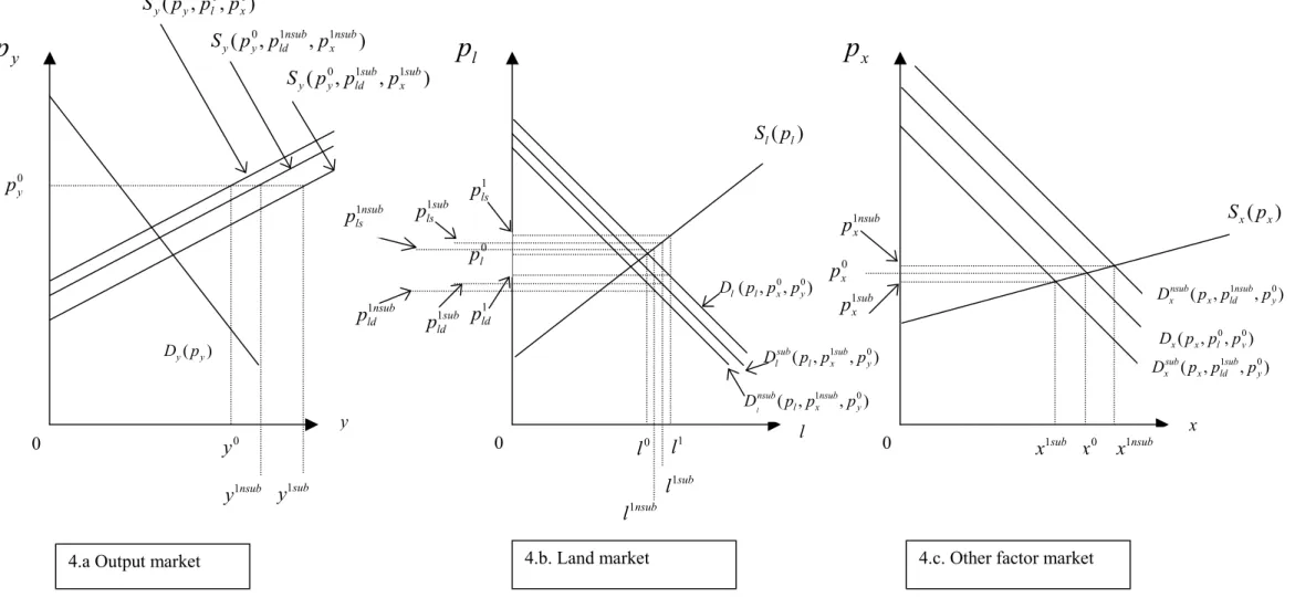
0 l p pl0 0 l l0 1 y y l l s p0− 1 l ) , ( y 0l y p p S ) , ( y l0 l y p p s S − ) ( _y y p D ( , ) 0 y l l p p D ) , ( 0 y l l p p D ) , ( _l 0_y sl _{p p} D l 0 0 0 ) ( _l l p S 1 l p l l s p0− ) ( _l l p S

The one output-two factor case: Illustrating the key role of factor substitution possibilities Let’s return to the case depicted by figure 2. We change only 2 assumptions. Firstly the considered support policy instrument is no longer output price support but a land subsidy. Secondly the supply of the other factor is now assumed to be imperfectly elastic. Therefore, the supply curve of this other factor is increasing in its price, as shown on figure 4, panel 4.c.

Figure 4 indicates that at initial equilibrium, the domestic output price is

p

0_y, the representative farmer produces quantity y0 using quantity l0 of land and quantity x0 of the other factor. The initial rental price of land is p_l0, while the initial price of the other factor is p_x0.

As in the above case, described by figure 3, the first incidence of the land subsidy is to decrease the buying-in price (or the opportunity cost) of land for the farmer. This first incidence is represented on panel 4.b by the decrease in the price “paid” by the farmer from p_l0 to p1_ld. This price decrease induces a rise in the farmer’s land demand (from l0 to l1) that, due to the relative scarcity of available land, implies an increase in the market (or supply) rental price of land up to p1_ls. As a result the land subsidy generates a gap between the demand and the supply rental prices of land (i.e., p_ls1 − p_ld1 =s_l). Following the reduction in the buying-in price of land the farmer’s marginal cost of production is going to decrease inducing a shift to the right of the output supply curve. However, this shift is not represented on panel 4;a at this stage because its extent closely depends on the range of substitution possibilities between land and the other factor.

- Let’s consider first the case where land and the other factor are highly substitutable. As the land subsidy makes the buying-in price of land to decrease, the farmer has incentive to substitute land to factor

x

in the production process. As the available technology allows such factor substitution adjustment the derived demand of factor

x

starts to decrease (the demand curve of factor

x

shifts to the left on panel 4.c). However, as the supply of factor

x

is imperfectly elastic the price of factor

x

starts to adjust down slowing down the substitution process between land and factor

x

. Hence at last a new equilibrium is reached where, as shown by panels 4.b and 4.c, both derived demand curves have shifted to the left due to factor price adjustment interactions (from

D

_l

(

p

_l

,

p

0_y

,

p

_x0

)

to

(

,

0

,

1sub

)

x y l sub

l

p

p

p

D

for land and from

)

,

,

(

_x 0_{y l}0

x

p

p

p

D

to

D

_xsub

(

p

_x

,

p

_y0

,

p

_ld1sub

)

for factor

x

). As both the buying-in price of land and the price of factor

x

have decreased following the land subsidy implementation the farmer’s marginal cost of production has lowered from the initial to the final equilibrium. Hence on panel 4.a the final output supply curve is

(

,

1

,

1sub

)

x sub ld y sub y

p

p

p

land subsidy induces an increase in output quantity from y0 to y1sub. This new equilibrium output quantity is obtained by combining an increased quantity of land (from l0 to l1sub) and a decreased quantity of factor

x

(from x0 to x1sub).

- Let’s consider now the situation where land and the other factor are hardly substitutable. In order to simplify the analysis and keep figure 4 readable we assume that land and factor

x

are complementary. In such a case, the first increase in land demand following the land subsidy implementation is accompanied by a simultaneous increase in the demand of factor

x

(since both factors are complementary). Hence on the factor

x

the price starts to rise. This price increase acts as to slow down, firstly the increase in both factor demands, secondly the lowering of the farmer’s marginal production cost (following the decrease in the buying-in price of land) and finally the expansion of output supply. Hence at last a new equilibrium is reached where on panel 4.a the final output supply curve is

S

_ynsub

(

p

_y

,

p

_ld1nsub

,

p

_x1nsub

)

and the output quantity y1nsub_{. This later is lower than y}1sub _{essentially because contrary to the above} “substitution case”, the complementarity between land and factor

x

in production prevents the farmer from exploiting fully the decrease in the buying-in price of land by substituting cheaper land to relatively more expensive factor

x

. As a result the output marginal cost of production decreases less in the “complementarity case” than in the “substitution case”. For the same reason, the new equilibrium quantity use of land l1nsub is lower than the one observed in the “substitution case”, but still higher than the initial level l0 (cf. panel 4.b). However, contrary to the “substitution case”, the factor complementarity relationship makes the land subsidy to induce an increase in the quantity use of factor

x

(from x0 to x1nsub on panel 4.c).

Finally, figure 4 shows that the effects of a land subsidy may be quite different according to the degree of factor substitution possibilities in production. First of all figure 4 indicates that a land subsidy may induce a decrease, no change or an increase in the quantity use and the market price of the non-land factors/inputs depending on to the range of substitution possibilities between land and non-land factors/inputs from strong substitutes to complements. Secondly, figure 4 shows that if the land subsidy unambiguously induces an increase in the output supply quantity, the extent of this increase closely depends on the degree of land and non-land factor/input substitution in production: the higher the substitution possibilities the greater the output supply increase. Thirdly, figure 4 indicates that if the land subsidy unambiguously induces an increase in the rental market price of land, a decrease in the corresponding buying-in price for the farmer and an increase in the land use quantity, the extent of these adjustments closely depends on the land to non-land factor/input substitution possibilities: the

higher the substitution possibilities the greater the increase in both the land use quantity and the rental market price of land.

It is interesting to point out at this stage that the overall support provided through the land subsidy is shared between the farmer, the landowner and the non-land factor/input supplier. Whatever the factor substitution possibilities, both the farmer and the landowner experience a gain resulting from respectively the decrease in the buying-in price of land and the increase of its market price. The gain for both agents is however greater when land and non-land factors/inputs are strong substitutes in production since in that case the benefit of support is not shared with the non-land factor/input supplier. Indeed in that case the non-land factor/input supplier may experience a loss, part of his/her surplus being transferred to the farmer via the decrease in the non-land factor/input price and to the landowner via the stronger increase in derived demand on the land rental market. At reverse and as shown by figure 4, when land and non-land factors/inputs are complements in production the non-land factor/input supplier may experience a gain that reduces the benefit for the farmer and the landowner. Finally, as regards the impact of the land subsidy on land rental market and price, one may synthesise the main findings as follows.

For given supply price elasticities of land and non-land factors/inputs, the higher the substitution elasticity between land and non-land factors/inputs:

- The higher the increase in the rental market price of land and the higher the amount of support “capitalised” in the rental price of land.

- The greater the decrease in the production cost of the output (and the higher the positive effect of the land subsidy on output quantity supply).

- The higher the gain of the farmer in terms of increased surplus and the higher the amount of support transferred to the landowner.

Comparing the effects of both the output price support and the land subsidy instruments one may draw the main following insights (still for given supply price elasticities of land and non-land factors/inputs):

- Both instruments are expected to increase output supply and for both instruments the higher the degree of substitution between land and non-land factors/inputs the greater the extent of the output increase.

- Both instruments are expected to increase land use and land rental price. For the output price support instrument, the higher the degree of substitution between land and non-land factors/inputs the lower the extent of land use and land rental price increases. At reverse, for the land subsidy instrument, the higher the degree of substitution the greater the extent of land use and land rental price increases. The main reason for this reverse impact of the substitution

possibilities lies in the differentiated first incidences of both instruments. The first incidence of the output price support instrument is to generate an incentive for the farmer to increase output supply. As expanding output requires using more factors/inputs, this first incidence then spreads within all factor and input markets. And the higher the substitution possibilities between factors/inputs the greater the dilution of support across factors/inputs. In other words the higher the substitution possibilities the less the support is allowed to concentrate on one specific factor or input (in our example, land). At reverse, the first incidence of the land subsidy is to decrease the buying-in price of land for the farmer. Hence, in this case the support initially concentrates on land and then spreads within the output and other factor/input markets. But the higher the substitution possibilities between land and non-land factors/inputs, the more the farmer can increase his/her land use and consequently the less the support is allowed to spread within non-land markets.

The previous graphical analysis does not allow to conclude about the comparative effect on output supply of the same amount of support given through either the output price support or the land subsidy instrument. However, Hertel (1989), Dewbre et al.(2001) and Guyomard et al. (2004) using different frameworks (and hence different assumptions) have obtained some analytical results to this regards.

- Under constant return to scale assumption, perfectly elastic supplies of non-land inputs and imperfectly elastic land supply, Hertel (1989) shows that an input subsidy will have greater impact on output supply than an equal cost output subsidy, provided the subsidised input substitutes for land. Contrary to our case, the subsidised input in Hertel’s study is not land but a non-land input with a perfectly elastic supply. And this is exactly because the subsidy is applied to an input with perfectly elastic supply that Hertel obtains the above presented result. - In Dewbre et al. (2001), the subsidy is alternatively applied to land and non-land inputs and

the supply of both categories of inputs may be perfectly/imperfectly elastic or perfectly inelastic. Under constant return to scale and small country assumptions, Dewbre et al. show that market price support will have greater impact on output supply than an equal cost land subsidy (or payment based on area) if the elasticity of supply of land is lower than that of the non-land inputs.

- In a more general framework (no constant return to scale assumption, no small country assumption, free entry and exit in the agricultural sector) Guyomard et al. (2004) show that an output subsidy will unambiguously have greater impact on output supply than an equal cost land subsidy. They also demonstrate that an output subsidy will unambiguously have lower impact on land rental price than an equal cost land subsidy. In other words, and conform to the intuition that arises from our previous graphical analysis, a larger part of support is

“capitalised” in the rental price of land when this support is provided through a land subsidy than through output price support.

At this stage, it is interesting to point out that the current evolution of agricultural policies in OECD countries is likely to reinforce the capitalisation of support in the farmland rental price. Indeed, according to Guyomard et al.’s result, the decapitalisation of support that should follow the decrease in the support based on output should be more than counterbalanced by the intensification of capitalisation of support that should follow the increase in support based on area. Of course, there are a lot of other factors that can influence the evolution of farmland rental prices in OECD countries (such as legal factors for instance, see e.g., Latruffe and Le Mouël, 2006). In addition, the land subsidy as designed in Guyomard et al. (2004) and in this report does not fit the much more complex area payment systems that some OECD countries have actually implemented (see discussion in point 2.1.4. below). However, this is a matter of fact that the current evolution of agricultural policies in OECD countries mainly consists in replacing market price support instruments through which the support is based on output and likely to “capitalise” less in farmland rental prices by direct payment systems through which the support is most often (explicitly or implicitly) based on area and likely to “capitalise” more in farmland rental prices.

Figure 4. Effects of a land subsidy on domestic output and factor markets: the two-factor case

4.a Output market 4.b. Land market 4.c. Other factor market

y

p

p

_l

p

_x y l x 0 y y 0 y

p

0 l p 0 x p 0 l l1 x0 y 1 ld p sub x1 ) ( y y p D ( , , ) 0 0 y l x x p p p D ) , , ( 1 0 y nsub x l nsub p p p D l ) , , ( 1 0y sub x l sub l p p p D ) , , ( 1 0y sub ld x sub x p p p D 0 0 0 sub y1 nsub y1 ) , , ( l 0x 0y l p p p D 1 ls p ) , , ( 1 0y nsub ld x nsub x p p p D sub l1 ) ( _l l p S ) ( _x x p S nsub x1 sub ls p1 nsub ls p1 nsub l1 sub ld p1 nsub ld p1 nsub x p1 sub x p1

)

,

,

(

0 1 1sub x sub ld y y

p

p

p

S

) , , ( 0 1 1nsub x nsub ld y y p p p S

)

,

,

(

_{y l}0 0_x y

p

p

p

S

2.1.3. factor supply price elasticities and substitution elasticities: Discussion

As shown by the previous graphical analysis, whatever the policy instrument used, the extent to which support is “capitalised” in the rental price of farmland closely depends on i) the level of the supply price elasticity of farmland relative to those of other agricultural factors/inputs and ii) the range of substitution possibilities between agricultural land and non-land factors/inputs in production.

What do these parameters mean and measure exactly? What do we know exactly about their respective values?

Factor supply elasticities: Indicators of the extent of mobility of factors

Let’s consider a representative landowner who owns the whole available land area in a country and whose objective is to maximise his/her revenue from renting out this land. Let’s first assume that the only possible use for this whole land area is agriculture and that the national agricultural sector produces only one output. In that case, the only way for the landowner to get back some revenue from his/her land is to allocate all available land to the agricultural sector. As there is not any alternative use for this available land, the quantity supplied will not depend on the land rental price. In other words, land is a specific factor to the agricultural sector and the supply price elasticity of land is at its lower bound level, i.e., 0 (land supply is perfectly inelastic). This first case characterises the situation where land is completely fixed and cannot move from agriculture to an alternative use.

Let’s assume now that there are two alternative uses for the whole available area, agricultural and non-agricultural uses. Hence the landowner is now able to split his/her available land between both uses so as to maximise his/her revenue. As a result, the quantity of land supplied to the agricultural sector will now vary according to the observed price on the rental market of farmland: an increase in this price, other things being equal, will lead the landowner to allocate more land to the agricultural sector. In other words, land is no longer a specific factor to the agricultural sector and the supply price elasticity of farmland becomes positive (farmland supply is imperfectly inelastic). This second case characterises a situation where land can move from agriculture to another use (land is mobile between alternative uses).

At this stage, one may wonder what makes land to be more or less mobile between alternative uses (or the level of the price elasticity of farmland to be more or less high)? There are at least to key factors to consider here.

The first one is technical and relates to the homogenous or heterogenous nature of land. Homogeneity means that all available hectares of land are identical (i.e., exhibit the same characteristics and so are of the same quality) and can be used equally in agriculture or in non-agricultural activity. In such a case, starting from a situation where the landowner faces equivalent rental prices for both possible

land uses, as soon as say the rental price of farmland becomes higher than the rental price of non-agricultural land there is no reason for the landowner not to allocate all his/her available hectares to agriculture. Hence homogeneity contributes to make land supply to each potential user sector very responsive to price changes. Conversely, heterogeneity implies that available hectares are different and do not suit equally to alternative uses. In that case, once the rental price of farmland increases relative to the one of non-agricultural land, the landowner will still have incentive to allocate more land to the agricultural sector but will be more constrained in doing so because his/her available hectares will be more and more difficult to convert to the agricultural use. In the extreme case where part of available hectares are well-suited only for agricultural use while the remaining hectares only suit for non-agricultural use, we return to the above first case: there are two types of land, each specific to one use, and supplied in fixed quantities to agriculture and non-agricultural activity. Finally the more homogenous the land, the higher the degree of mobility between alternative uses and the higher the elasticities of land supply to each user sector.

The second key factor as regards the extent of land mobility across alternative uses relates to land management laws and policies in force in most countries that most often prevent landowners to convert their land from agricultural to non-agricultural uses. OECD (1996) and Latruffe and Le Mouël (2006) for example show that in most OECD countries there are planning or zoning legislations that designate land as farmland, building land, etc. and there are laws that prevent converting land from its administratively designated use to alternative uses. This is particularly true for agricultural land which is highly protected from the competition of other uses in a lot of OECD countries. Such legislations clearly contribute to lower land mobility across alternative uses, especially farmland mobility from the agricultural to other sectors. Therefore the stricter the legislation as to protect agricultural land from competing uses, the lower the degree of mobility of farmland between agriculture and other sectors and the higher the elasticity of supply of farmland.

Finally, one may advocate the case where the agricultural sector produces more than one output. This case is in fact very close to the situation described above where the two alternative uses of land would be two agricultural uses, say crop and livestock for instance. In that situation, if the role of land management laws and policies would likely to be less important as regards the extent of land mobility, the later would continue to closely depend on the degree of land homogeneity.6 At this stage one

6

Such laws and policies usually apply to the whole agricultural land and therefore essentially affect the extent of land mobility between agricultural and non-agricultural uses. Most often they are not designed as to protect specific agricultural land uses (say crop) from competing agricultural land uses (say livestock). One may underline however that in many countries there are actually legal provisions that prevent converting specific agricultural land areas (environmentally sensitive areas for example) to certain agricultural uses (intensive

guesses easily that land is likely to be more homogenous when considering two alternative agricultural uses than when considering an agricultural use vs. a non-agricultural use. In other words, it is likely that the elasticity of land supply to the crop sector is higher than the elasticity of land supply to the agricultural sector as a whole and it is even more likely that the elasticity of land supply to the grain production sector for instance is higher than the one to the whole agricultural sector.

If the above statement gives some indication about the ranging of land supply elasticities according to the overall possible uses of land, it says nothing about the expected values of these parameters. Indeed one must admit that we know nothing about the values of these parameters since there are no available land supply elasticity estimates in existing literature (e.g., OECD, 2001). One expect that these parameters differ across countries (and even across regions within countries) since firstly available land in countries is more or less homogenous due to observed natural and weather conditions, secondly land management laws and policies differ across countries.

It is commonly admitted that the elasticity of land supply to the agricultural sector is very low, at least in OECD countries. And this is globally the only available information on land supply elasticity parameters. Therefore, most global simulation models centred on agriculture assume no land mobility between agriculture and other sectors in national economies, that is a perfectly inelastic supply of agricultural land (i.e., a zero elasticity).

It is also commonly admitted that amongst all factors/inputs used in agriculture, land is likely to be the less mobile from agricultural to non-agricultural uses. Hence at the whole agricultural sector level, land supply elasticity is probably lower than supply elasticities of all other factors/inputs. Common knowledge about agriculture in OECD countries is that family labour is the second factor that is likely to be hardly mobile between agriculture and other sectors. Usually it is recognised however that family labour is likely to be more mobile than land. Hence, at the whole agricultural sector level the supply of family labour is likely to be imperfectly elastic, but with a higher elasticity than land supply. Finally, it is also well-admitted that all other factors/inputs are likely to be very mobile between agriculture and other sectors, at least and once again in OECD countries. Hence supplies of these other factors/inputs are, always in theoretical models and most often in global simulation models, assumed to be perfectly elastic (i.e., an infinite elasticity).7

What does it mean as regards the effects of policy support instruments? As shown by the previous graphical analysis, whatever the used policy instrument the higher the supply elasticity of a factor the higher the share of support “capitalised” in its market price. Hence it is likely that:

7

Usually, the same ranging is adopted regarding the mobility of factors/inputs within the agricultural sectors, but with all elasticity values moving up to higher levels indicating that land, family labour and, to a lesser extent, other factors/inputs are more mobile across alternative agricultural uses than across agriculture and other uses.

- a significant share of agricultural support in OECD countries is “capitalised” in the rental price of farmland;

- family labour also benefits from agricultural support but to a lesser extent than land and particularly when support is provided through output price support instruments;

- when support is provided through a land subsidy a larger share of support is “capitalised” in the price of land while family labour may be hurt if land is a sufficiently strong substitute to family labour in production.

Elasticities of substitution: Indicators of the flexibility of the technology

Neoclassical production theory recognises the possibility of substituting one factor/input to another. The degree to which one factor/input may be substituted to another is implicitly determined by the form of the production function. The elasticity of substitution between two factor/inputs measures, for a cost-minimising producer, the percentage change in the ratio of both factor/input uses per percentage change in the ratio of their prices.

There are two important features here. First of all, the elasticity of substitution is defined for a cost-minimising producer. This means that the elasticity of substitution is defined for a given output quantity. In other words the elasticity of substitution indicates how the relative uses of two factor/inputs vary when their relative prices vary, keeping constant the output quantity produced. Secondly, there is a crucial difference between the definition of the elasticity of substitution when moving from a 2-factor/input framework to a n-factor/input framework. The elasticity of substitution is defined for pairs of factor/inputs. Hence when dealing with more than two factor/inputs, the elasticity of substitution between factor/input i and factor/input j is partial, meaning that it measures the percentage change in the ratio of used quantities of i and j per percentage change in the ratio of their prices, holding constant all other factor/inputs. Therefore, in a n-factor/input framework, the elasticities of substitution do not represent the full degree of substitution possibilities present in the production function.

At reverse to previous factor supply price elasticities, one can find numerous estimates of elasticities of substitution between factor/inputs used in agricultural production. This is obviously out of the scope of this study to make a review of these estimates. OECD (2001) provides an extensive review of available estimates of elasticities of substitution in agricultural production for Canada, the European Union, Mexico and the US. This review was carried out in the course of the development of the PEM model as to support the parameter calibration stage.

- at aggregate agricultural level, broad categories of factor/inputs (mainly land, family labour, capital and purchased inputs, such as hired labour, fertilisers, pesticides, seeds, energy, etc.) are in average found to be rather substitutes than complements in production;

- at aggregate agricultural level, land is likely to be stronger substitute with purchased inputs than with family labour and/or capital;

- however estimates vary widely across studies, pairs of factor/inputs sometimes moving from strong substitutes to strong complements.

What does it mean as regards the effects of policy support instruments? The main insight here relates to the current evolution of agricultural policies in OECD countries, i.e., the shift from output price support instruments to factor (especially land) subsidy instruments. Provided that land is rather a substitute to other factor/inputs in agricultural production, it is likely that output price support was spread within all factor/input markets through the game of substitution in production, allowing factor/inputs with imperfectly elastic supply (family labour for example) to benefit from support to the detriment of the “capitalisation” in the rental price of land. The shift from price support to land subsidy instruments is likely to play conversely. More specifically, provided that land is a substitute to other factor/inputs in agricultural production, it would be able to “retain” a larger share of support, the later being driven towards the subsidised factor through the game of substitution in production. In such a case, family labour is likely to benefit less from the support provided through a land subsidy. At this stage, one guesses that the way the land subsidy system is designed and particularly who is the beneficiary (the farmer or the landowner?) and under which conditions the subsidy is given are crucial elements as regards the sharing out of support between imperfectly mobile agricultural production factors (i.e., mainly farmland and family labour).

2.1.4. Some modelling issues

All existing global simulation models centred on agriculture (of either partial or general equilibrium nature) may be considered as elaborated versions of the very simple models we adopted throughout the above graphical analysis. They all rely on implicitly or explicitly specified agricultural (and, in multi-sector or general equilibrium models, other sectors’) production functions and on supply functions of production factors (resulting from optimisation behaviours of factor owners, either part of the model itself or considered as outside from the model). The main difference is of course the number of considered outputs and factor/inputs. As a result, much more markets are simultaneously responding to an exogenous (policy) shock, making much more difficult to predict the outcomes.8

8

Another important difference with respect to the basic models used in our graphical analysis is that global simulation models most often consider several countries, some of them assumed to be large countries. Hence, an