HAL Id: halshs-01472039
https://halshs.archives-ouvertes.fr/halshs-01472039
Submitted on 20 Feb 2017HAL is a multi-disciplinary open access
archive for the deposit and dissemination of sci-entific research documents, whether they are pub-lished or not. The documents may come from teaching and research institutions in France or abroad, or from public or private research centers.
L’archive ouverte pluridisciplinaire HAL, est destinée au dépôt et à la diffusion de documents scientifiques de niveau recherche, publiés ou non, émanant des établissements d’enseignement et de recherche français ou étrangers, des laboratoires publics ou privés.
Guillaume Le Roux, Julie Vallée, Hadrien Commenges
To cite this version:
Guillaume Le Roux, Julie Vallée, Hadrien Commenges. Social segregation around the clock in the Paris region (France). Journal of Transport Geography, Elsevier, 2017, 59, pp.134-145. �10.1016/j.jtrangeo.2017.02.003�. �halshs-01472039�
1
Social segregation around the clock in the Paris region (France)
Summary
While social scientists have invested a lot of energy in exploring the uneven distribution of social groups in the city, they have surprisingly limited their efforts to investigating social segregation at the place of residence. The present paper investigates social segregation over the 24 hours a day in the Paris region, taking into account how social groups move within a city throughout the day.
From a large and precise daily travel survey carried out in the Paris region (EGT 2010) among 25,500 respondents aged 16 or over, we have computed segregation indices and maps hour by hour from respondents’ educational and socioprofessional indicators. We then observed that social segregation within the Paris region decreases during the day and that the most segregated group (the upper class group) during the night remains the most segregated during the day. We also explored how the co-presence between various social groups evolves throughout the day. Finally, we highlighted some large variations in districts’ social composition over 24 hours: districts with similar social composition during the night can differ deeply in their social composition during the day-time because of socially selective daily trips.
Exploring social segregation around the clock helps in considering more dynamically place effects on individual behavior and targeting areas to implement interventions more connected with the real city rhythm.
Keywords: social segregation, daily mobility, travel data, activity-based approach
Highlights
- Segregation around the clock was explored from a travel survey (Paris region). - At city scale, social segregation is lower during the day than during the night. - The upper class is the most segregated group during the night and the day. - At local scale, large variations in districts’ social composition occur over a day. - Daily trips which are socially and spatially selective alter maps of social groups.
2
1 Context
1.1 Research justification
The present paper investigates social segregation (defined as the uneven spatial distribution of social groups) over the 24 hours a day within a metropolitan area, taking into account how social groups move within a city throughout the day. At least three reasons support the importance of exploring social segregation around the clock. Firstly, neighborhood attributes and neighborhood effects both have to be considered dynamically, taking into account population daily mobility. When moving, inhabitants may indeed be exposed to different neighborhoods and social contexts and, conversely, transform the social context of inhabitants who do not move (Wong and Shaw, 2011). Education, employment, or health issues could then be related not only to residential segregation (“night-time” segregation), but also to “day-time” segregation. Secondly, public and municipal actors may find it more efficient to implement interventions in areas with high concentrations of specific social groups not only during the night but also during the day. Crossing information about night-time and day-time segregation would then be useful for every action aiming to reduce social inequalities in the city. Finally, social segregation around the clock may also contribute to the enhancement of urban models of social structures and dynamics. Debates about “fragmented cities” (Borsdorf and Hidalgo, 2009) or “villes éclatées” (May et al., 1998) integrate notions such as social and spatial cohesion and exclusion, but few quantitative analyses consider how social groups mix or are isolated in a city on a daily basis.
1.2 A brief combined review of segregation and daily mobility
Social scientists have invested a lot of energy over a number of decades into measuring properly the uneven distribution of social groups in the city. For a long time, scientific debate about segregation was focused on the bias and redundancy of segregation indices (Hornseth, 1947; Jahn et al., 1947; Williams, 1948; Jahn, 1950; Cowgill and Cowgill, 1951), on the weaknesses of the index of dissimilarity (Cortese et al., 1976; Taeuber and Taeuber, 1976; Massey, 1978; Massey and Denton, 1988), or on the development of spatially-aware measures of segregation (Grannis, 2002; Reardon and O’Sullivan, 2004; White, 1983; Wong, 2005). However, they have, surprisingly, limited their efforts to investigating segregation at the place of residence and have not explored the geography of social groups during the day-time. Even if the term “occupational segregation” was introduced earlier in the literature, it was only to designate either the uneven residential distribution of occupation groups (Duncan and Duncan, 1955) or the uneven distribution of sociodemographic groups (mainly male versus female) among occupational categories without spatial consideration (Abrahamson and Sigelman, 1987). While census data could have been used to measure workplace segregation, empirical studies on workplace segregation are scarce and relatively new (Hellerstein and Neumark, 2008; Åslund and Skans, 2010). Investigating the characteristics of co-workers at an establishment-level in US or Swedish cities from employment databases, these studies produced valuable information on ethnic segregation patterns but did not provide information on the day-time localization of social groups within the city. In that vein, the study by Ellis et al. (2004) has to be mentioned. The authors compared levels of residential and work tract segregation for native and immigrant groups in Los Angeles; however, focusing on the working-class population, they do not consider people that are not working nor the effect of other kinds of daily activity (leisure, shopping, etc.).
3 For a long time, studies about day-time population (Chapin and Stewart, 1953; Foley, 1952, 1954) have been ignored in segregation literature. Mechanisms of segregation and of daily mobility could yet benefit from being combined: daily mobility is socially differentiated according to socio-demographic characteristics, as highlighted by Orfeuil’s daily mobility state of the art (2002), and can either promote interactions between different social groups, as suggested in more and less recent literature (Park, 1925; Urry, 2002), or, on the contrary, reinforce avoidance practices or affinity aggregation of certain social groups (Chamboredon and Lemaire, 1970; Authier, 1993).
Only recently, several authors have explored urban segregation from an activity-based approach. For this purpose, time-geographic analysis methods have been developed to compare the shapes of activity spaces for members of distinct social groups. This first type of work focuses on the socio-spatial isolation of agents, as developed by Lee and Kwan (2011) for Koreans in Columbus (USA). Another group of papers takes into account the social characteristics of places crossed in people’s activity spaces. They assess the exposure of members of different social groups to other social groups in respect of the spaces in which they conduct their everyday life. For example, to study ethnic segregation in southeast Florida, Wong and Shaw (2011) proposed an exposure measure using a travel survey to implement activity spaces and census data to socially qualify the visited neighborhoods. With the same kind of approach and using information on daily mobility from a health survey, Krivo et al. (2013) showed for socioeconomic and ethnic groups in Los Angeles that residents of both advantaged and disadvantaged neighborhoods experience social isolation when they travel through the city to conduct their daily activities. Nevertheless, these studies face the limitation of considering the social composition of crossed neighborhoods in the activity spaces according to resident characteristics and not their variations during the day. Transcending this limitation, recent studies have taken into account the dynamics of space by using large travel surveys or mobile phone datasets. Palmer (2013), for example, proposed a range of “activity-space segregation indexes” derived from well-tested residential segregation indexes but taking into account individual daily schedules and the time spent in the different census tracts. In a similar vein, Silm and Ahas (2014) described the spatiotemporal variation of segregation indexes computed from a mobile phone dataset for Russians living in Tallinn (Estonia). They identified significant differences in the level of segregation of the group according to the hour of the day, weekdays and weekends, and seasonal rhythms. Finally, Farber et al. (2015) proposed a reproducible exposure measure based on potential opportunities for social contact for members of different social groups by taking into account the intersection of their spatiotemporal activity patterns.
1.3 Objectives
Following a similar activity-based approach, the present paper explores social segregation around the clock in the Paris region using a large daily travel survey carried out in the Paris region among 25,500 respondents aged 16 or over. Four objectives can be distinguished here.
First, we aim to compare classic measures of “night-time” segregation (residence-based) with measures of “day-time” segregation (activity-based). The previous few papers dealing with this question underlined that ethnic segregation decreases significantly during the afternoon in the capital of Estonia (Silm and Ahas, 2014) or when comparing work tract segregation and residence tract segregation in Los Angeles (Ellis et al., 2004). Do we observe similar findings
4 about social segregation in the Paris region? Are there some specific periods during the day in which segregation is especially low or high?
The second objective of the paper is to identify the most segregated group, not only during the night, but also during the day. While urban segregation and deprivation are often linked in many public policy statements, some studies in Paris (Préteceille, 2006) and in other European cities (Musterd, 2006) have shown from residential-based data that the upper class is the most segregated group. Do daily trips, which are socially differentiated in terms of distance and type of activity, also give the upper class “the award” of the most segregated group during the day? In a third step, we explore social segregation over 24 hours from the co-presence of various social groups in the same urban areas. Term of “co-presence” - defined as simultaneous presence of individuals in the same place - has been preferred to the term of “interaction” (often used in some quantitative segregation studies) since spatial proximity between social groups does not imply necessarily social contacts or real interactions (Chamboredon and Lemaire, 1970). Qualitative work on the French bourgeoisie showed how the dominant class promotes living with peers and deliberately keeps other social classes away from its favorite places (Pinçon and Pinçon-Charlot, 2007). How strongly does the upper class keep its distance from other social groups when they carry out their activities during the day, and do these behaviors extend to other social groups? Do probabilities of co-presence between upper and lower class members remain similar over a 24 hour period? At what time co-presence probabilities are the lowest?
Lastly, our analysis of social segregation around the clock aims to pinpoint areas with substantial changes in their population’s social composition over 24 hours. While spatial distribution of social groups in the Paris region, organized around a west/east division, is now fairly well known (Préteceille, 2006), some studies focusing on particular neighborhoods have underlined how far visiting populations may differ socially from resident populations and how strongly the non-resident populations may contribute to the social labeling of some areas - for example, in the case of the Château-Rouge neighborhood in Paris (Chabrol, 2011). How do socio-spatial divisions, traditionally observed from residential-based data, evolve around the clock?
2 Data
2.1 Household travel survey
The Enquête Globale Transport (EGT) is a large household travel survey carried out every ten years in the Paris region (Ile-de-France) since 1976. In the present paper, we used the last edition (EGT 2010, STIF-OMNIL-DRIEA) which took place during two periods: from October 2009 to May 2010 and from October 2010 to May 2011 (i.e. over 16 months of surveys). This survey provides a large amount of information on the daily mobility of inhabitants aged five and older, in addition to household and individual characteristics.
About 15,000 households were selected and surveyed about their trips on weekdays (Monday to Friday) and 3,000 about their trips at weekends (Saturday or Sunday). Data from more than 43,000 respondents (and 18,000 households) were collected, with a total of 143,000 trips.
5 In the present research, we took into account respondents aged 16 years or over, considering that younger people were not sufficiently autonomous in their daily mobility (Massot and Zaffran, 2007). Of the 26,312 respondents during the week aged 16 or over, 813 were excluded due to missing data in their daily mobility schedule or in socioprofessional or educational status. The final sample contains 25,499 respondents aged 16 or over with a total of 101,814 weekdays trips and 127,245 locations.
In EGT sample design, the Paris region has been subdivided into 109 districts (“secteurs”). They correspond to groups of municipalities or arrondissements in Paris and consist of approximately 100,000 inhabitants. Smaller in inner Paris and larger in the peripheral areas, their sizes vary from 3 to 1,326 km2 (with a median area of 14 km²). Districts are the primary sampling units in EGT survey: in every district, 400 to 500 residents have been surveyed among randomly selected households to ensure reliable estimates at district scale. In the present paper, district scale was then chosen to investigate variation around the clock in social composition within the Paris region.
Weighting coefficients in the 2010 EGT survey were computed at household and individual levels to afford every district the same distribution in household profile (size and housing type) and population profile (age, sex, occupation, and socioprofessional group) as the distribution observed in the 2008 French census. Every analysis presented in the present paper has been made taking into account these weighting coefficients.
2.2 From trip dataset to location dataset
Every trip starting and/or ending in the Paris region made the day before the survey was reported by respondents. Following trip variables were available: precise localization of place of departure and place of arrival (using a 100 square meters grid cell), time of departure and time of arrival (with exact minutes), trip purpose and mode of transportation used. For the present analysis, the trip dataset was transformed into a location dataset in which (1) every location was defined at district scale (i.e., the smallest scale which it is possible to aggregate results, due to the EGT sample design) and (2) 24 hourly time steps are defined for taking 24 cross-sectional pictures of individuals' location.
To reduce spatiotemporal heterogeneity between trips occurring on weekends and on weekdays (Buliung et al, 2008), we restricted our dataset to weekday trips. As in many transportations studies, we considered weekday trips as occurring an “average working day” even if there may be some intrapersonal variability in travel behavior between days of the week (Monday to Friday) and period of the year (Pas, 1987). As EGT survey took place from October to May, variability related to summer time was excluded.
We kept trips occurring between 4:00 am (day before survey) and 3:59 am (day of survey) and removed trips outside this window. Individuals who reported staying at home all day were assigned to their district of residence over the entire observation period. Individuals were moved to a fictive place, “in transportation”, when they were moving except if they used an “adherent” mode of transportation (Amar, 1993), such as walking and non-motorized modes. In such cases, half of the trip was considered as located in the district of origin and the other half as located in the district of destination. This choice was motivated by the fact that people using
human-6 powered modes of transportation actively contribute to social interactions and social labelling of spaces.
2.3 Social indicators
2.3.1 Description
From EGT data about respondents’ achieved level of education (initially in ten groups), we computed a first social indicator corresponding to the lowest level of education of the adults in the household. Called ‘educational status’, this variable was composed of four groups: low (middle school or less), middle-low (high school without Baccalauréat), middle-high (Baccalauréat to two years after Baccalauréat), and high (three years or more after Baccalauréat).
With the same educational data, we computed a second variable (continuous) from the mean number of years of study achieved by every adult in the household, called ‘scholarship duration’.
From respondents’ socioprofessional EGT data (initially in 24 groups, which were combined and ranked), we computed a social indicator corresponding to the lowest socioprofessional category of the adults in the household. Called “socioprofessional status”, this variable was composed of five groups: unemployed (unemployed long term, housework); low (workers and domestic services); middle-low (employees, craftsmen); middle-high (intermediary professionals, merchants, farm operators); and high (managers, intellectual professionals, employers of more than ten employees).
EGT (2010) also provided information about the households’ incomes but the rate of missing data (more than 20%) was too important to be used here to explore social segregation.
2.3.2 Methodological choices
Instead of computing social indicators from an individual point of view, we used the household level. Both approaches can be discussed (Chenu, 2000), but individual’s behavior is influenced by the context in which they are socialized, notably the household as a unit sharing social and economic resources. Social position may then sometimes be more relevant when computed at the household level: when focusing on conditions of life, lifestyles, or life chances, members of the same family or household unit should be assumed to share the same social position as they influence each other’s’ individual social position (Sørensen, 1994).
We decided to keep the lowest (and not the highest) educational status and socioprofessional status in the household for two reasons. First, educational or socioprofessional groups issued from “lowest procedure” have been found to be more correlated with the household’s income (when available). Second, the four educational groups issued from “lowest procedure” were found to be more evenly distributed than those issued from “highest procedure”. In initial EGT database, respondents whose level of education was “three years or more after Baccalauréat” were gathered in a same educational category. Such aggregation would lead to get a high educational category with nearly the half of the population (44%) if “highest procedure” would be used.
7 In socioprofessional status, the “unemployed” category (which consists of people living in a household where at least one adult is unemployed) refers to a large variety of situations. It includes, for example, households in which every adult is unemployed as well as households in which one adult has a highly qualified job and another adult doing housework. Despite such (relatively common) heterogeneity in the “unemployed” category, segregation according to socioprofessional status was interesting to investigate, to compare with segregation according to educational status and to discuss with findings from other studies.
2.4 Description of the sample
The final sample was composed of 25,499 respondents aged 16 or over with 101,814 trips. The number of respondents per district of residence varied from 124 to 406, with a median of 229. The studied population was predominantly female (52.9%) and of working age (Table 1). Social indicators related to socioprofessional status and educational status were well distributed across the population. The median value of scholarship duration was 12 years.
Table 1: Sociodemographic characteristics of the sample
N weighted %
Sex Male 11946 47.1%
Female 13553 52.9%
Age (in years)
16–29 4820 18.4% 30–39 5710 22.0% 40–49 5149 20.1% 50–64 6074 23.7% 65 and over 3746 15.8% Socioprofessional status*
Unemployed (unemployed long term, housework) 3105 14.6%
Low (workers and domestic services) 5970 22.5%
Middle-low (employees, craftsmen) 5576 21.2%
Middle-high (intermediary professionals, merchants, farm operators) 6686 24.4%
High (managers, intellectual professionals, employers of more than ten employees)
4162 17.3%
Educational status*
Low (middle school or less) 5170 21.0%
Middle-low (high school without Baccalauréat) 7293 27.2%
Middle-high (Baccalauréat to two years after Baccalauréat) 6954 26.5%
High (three years or more after Baccalauréat) 6082 25.3%
Source: EGT, 2010 (STIF-OMNIL-DRIEA) Note: * Lowest level among household’s adults
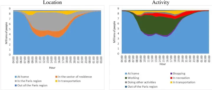
Figure 1 shows temporal counts of people aggregated according to their location and activity type. Such graphical displays have been used often in recent demographic studies (Billari, 2001), but there are also some examples in earlier studies (Jones and Clarke, 1988). We observe a marked morning peak hour between 8:00 and 9:00 and a smoothed afternoon peak hour between 17:30 and 19:30, along with a light peak of return home trips between 12:00 and 14:00. This tongue-shaped figure is consistent with other studies dealing with time use and activity-based travel demand (Carlstein et al., 1978; Goodchild and Janelle, 1984). Commuting trips structure the aggregated pattern in the location graph, since two thirds of individuals leaving home go out of their district of residence, most of them to work or study. The proportion of
8 recreational activities is significant from the afternoon onward and even becomes the most important reason for leaving home after 18:00.
According to these patterns, three time periods can be distinguished: night-time (23:00 to 8:00), when people are at home; day-time (8:00 to 18:00), when most people are working; and evening (18:00 to 23:00), as a transient period during which recreational activities are the most frequent out-of-home activities. These three periods will be used to compute specific indicators for district classification (see below).
Location Activity
Figure 1: Location and activity of the population aged 16 or over according to the hour of the day (working day)
Source: EGT, 2010 (STIF-OMNIL-DRIEA)
3 Methods
3.1 Indices of segregation
From the EGT dataset location, segregation indices were computed hourly (from 4:00 am to 3:00 am) regardless of the day of the week. If individuals were in transportation (not “adherent”), they were removed from the calculation. Among the panel of segregation indices commonly used in such works (Massey and Denton, 1988), we selected some for our research question in the light of their mathematical properties, their complementarity to measure different dimensions of segregation (evenness, concentration, exposure, centrality or spatial clustering) and their potential to consider social groups simultaneous (multigroup indices) or separately (unigroup indices).
3.1.1 Multigroup indices
To assess the extent of social segregation within the city by considering together the different social groups, we have selected two multigroup indexes (Reardon and Firebaugh, 2002): the Gini index and the information theory index. The first is a measure of disproportionality that emphasizes how groups are disproportionately represented in each spatial unit; the second is a
9 measure of diversity that assesses the degree of social mixity within the spatial units. Both vary between 0 (no segregation) and 1 (maximum segregation).
The formula of the Gini index is:
𝐺 = 1 2𝐼∑ (𝜋𝑚 𝑀 𝑚=1 ∑ (∑ 𝑡𝑖𝑡𝑗 𝑇2 |𝑟𝑖𝑚− 𝑟𝑗𝑚|)) 𝐽 𝑗=1 𝐽 𝑖=1
where: I is the Simpson’s interaction index ∑𝑀𝑚=1𝜋𝑚(1 − 𝜋𝑚) M is the number of social groups
𝜋𝑚 is the proportion of the population of group m J is the number of spatial units
𝑡𝑖 is the population in the spatial unit i T is the total population
𝑟𝑖𝑚 is the proportion of individuals from group m within the spatial unit i The information theory index is the weighted difference between the entropy of each spatial unit and the entropy of the whole city. The formula is:
𝐻 = ∑ 𝑡𝑗
𝑇𝐸(𝐸 − 𝐸𝑗) 𝐽
𝑗=1
where: E is the entropy index ∑𝑀𝑚=1𝜋𝑚𝑙𝑛(1/𝜋𝑚)
𝜋𝑚 is the proportion of the population of group m J is the number of spatial units
𝑡𝑖 is the population in the spatial unit i T is the total population
𝐸𝑗 is the entropy index of the spatial unit j
3.1.2 Unigroup indices
To assess the extent of social segregation for each social group, we crossed two indexes: the first (Duncan’s dissimilarity index) gave information about the dispersal of every social group across spatial units and the second (Moran’s index) is a measure of spatial autocorrelation of social groups within the city. Reporting values of these two unigroup indices on horizontal and vertical axes, we built a chart - sometimes called a segrograph (Girault and Bussi, 2001) - to investigate how segregation of social groups evolved over 24 hours.
Duncan’s dissimilarity index is commonly used as a measure of pairwise segregation (e.g. Black versus White) but it can also be used when measuring segregation of a social indicator divided in more than two groups. In this case, Duncan’s dissimilarity index expresses the proportion of individuals of a given social group who would have to change their spatial unit (without replacement) to get an even distribution of the group relative to the total population.
10 The formula used is:
𝐷 =1 2∑ | 𝑥𝑖 𝑋− 𝑡𝑖−𝑥𝑖 𝑇 − 𝑋)| 𝐽 𝑖=1
where:
𝑥
𝑖 is the population of the group in the spatial unit i X is the total population of the groupJ is the number of spatial units
𝑡𝑖 is the population in the spatial unit i T is the total population
Moran’s index is a measure of spatial autocorrelation. Its values vary from -1 (the group perfectly repulses itself) to 1 (the group is perfectly clustered in space), and a zero value indicates an absence of spatial structure. Moran’s index applied to the distribution of a social group equals:
I = J
∑𝐽𝑖=1∑𝐽𝑗=1𝑤𝑖𝑗
∑𝐽𝑖=1∑𝐽𝑗=1𝑤𝑖𝑗(𝑟𝑖− 𝑟̅)(𝑟𝑗− 𝑟̅) ∑𝐽𝑖=1(𝑟𝑖− 𝑟̅)2
where:
𝑟
𝑖 is the proportion of the population of the group in the spatial unit i 𝑟̅ is the mean of the proportion of the population of the group in the spatial unitsJ is the number of spatial units
𝑤
𝑖𝑗 equals 1 if spatial units i and j are neighbours, otherwise 03.1.3 Co-presence
A last index was used here to assess co-presence of social groups in the same spatial units. Bell’s index (1954) expresses the probability that a randomly chosen member of group X shares the same spatial unit than a member of group Y [xPy]. It is equal to the probability that a member of group Y shares the same spatial unit than a member of group X [yPx] only if the two groups X and Y have the same population size. To take into account potential differences in group size population and to get then symmetric indices, the probability that a randomly chosen member of group X is in the same spatial unit than a member of group Y was divided1 by the proportion of group Y in the population Y and X. Then, the adjusted index [xP*y] equals 0 if there is no co-presence of members of group X and Y in the same spatial units and equals 1 if members of groups X and Y are in the same proportion in every spatial unit and totally isolated from members of the other social groups.
1 Adjustment methods commonly used in the literature (e.g. Bell, 1954; White, 1986) suggest to divide Bell’s
index by the proportion of the group Y in the total population. However, when this adjustment method was applied to data categorized in more than two groups, the resulting index was not found to vary in the range [0; 1]. Actually, this adjustment method postulated that the maximum value of Bell’s index is the proportion of group Y in the population, which is true in the case of a population divided in two groups but false for a segmentation in more than two groups. This point seems to be ignored in the literature concerning Bell’s index.
11 Then, the formula used is:
𝑥𝑃∗𝑦 = 𝑋 + 𝑌 𝑌 ∑ 𝑥𝑖 𝑋 𝐽 𝑖=1 y𝑖 t𝑖
where:
𝑥
𝑖 is the population of the group X in the spatial unit i𝑦
𝑖 is the population of the group Y in the spatial unit i X is the total population of the group XY the total population of the group Y J is the number of spatial units
𝑡𝑖 is the population in the spatial unit i
3.1.4 Estimates, confidence intervals and tests of significance
As performed in other studies (Palmer, 2013), bootstrap methods (by randomly sampling our data 1000 times with replacement) were used to estimate means and 95% confidence intervals of Gini’s, Information Theory’s, Duncan’s and Adjusted Bell’s indices. Moreover, a Monte Carlo permutation test (R=1000) has been used to assess Moran’s autocorrelation index statistical significance at a level of 5% (Cliff and Ord, 1981). These methods provide estimates of the variance of the sampling distribution of each index and thus the potential error in any given estimate. However, they remain imperfect to provide unbiased estimates of the population index value from activity travel surveys (see Cools et al , 2010; Palmer, 2013 for extensive discussion).
3.2 District classification
To sum up the diversity of social dynamics throughout the day at district scale, principal component analysis (PCA) was computed from 13 district variables. Final district classification was obtained with hierarchical clustering. PCA was used to extract key information from highly correlated variables, particularly social level and social mixity indicators.
District indicators describing social profile and changes over 24 hours according to individuals present in the district were considered: (1) average value of scholarship duration; (2) average entropy index of educational status; (3) range value (maximum–minimum) of scholarship duration (% of average over 24 hours); and (4) range value (maximum–minimum) of the entropy index of educational status (% of average over 24 hours). Moreover, we also took into account district indicators describing changes between the three following time slots: night-time, from 23:00 to 8:00; day-night-time, from 8:00 to 18:00; and evening, from 18:00 to 23:00. These time slots were chosen according to the aggregated behaviors of daily mobility in the Paris region (see section 4.2, Figure 1). For every time slot, we computed: (1) rate of change2 (in %) of scholarship duration; (2) rate of change (in %) of the entropy index of educational status; and (3) rate of change (in %) of population number. For the computation of district indicators describing changes between time slots, individuals were weighted according to their duration of stay in the district during each time slot: for example, an individual who spent twice
12 as long as another in a district during a time slot contributed double to the district social composition during this time slot.
4 Results
4.1 Social segregation in the city around the clock
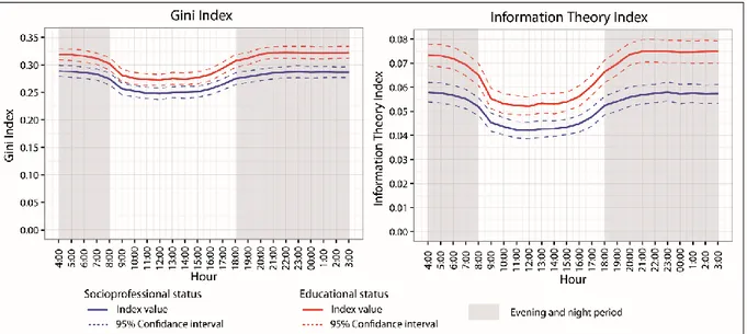
Segregation indices vary throughout the day (Figure 2): their values were found to be significantly higher during the night (from 21:00 to 5:00) than during the day (between 9:00 and 16:00). The Paris region is then less segregated during the day than during the night. When comparing maximum and minimum values, the Gini index is found to decrease by 15% and the information theory index by 30%. The decrease in segregation indexes in the evening is slower than the increase in the morning, which may be linked with the daily mobility rhythm observed in Figure 1 (departures from home in the morning are more condensed within specific hours than returns in the evening).
From a more methodological point of view, we can observe that: (i) indices computed from educational status were systematically higher than those computed from socioprofessional status, but evolution of their values over 24 hours was very similar; and (ii) the two segregation indices (Gini and information theory) gave similar shapes even if values from the information theory index (which focuses on social diversity in the districts) decrease relatively more during the day-time than those from the Gini index (which measures overrepresentation of groups in the districts). This suggests that the strongest phenomena occurring during the day is the increasing social diversity within the districts.
Figure 2: Variation of social segregation indices in the Paris region around the clock
13
4.2 Various patterns of segregation in the city around the clock according to social groups
Values of the unigroup segregation index (Duncan’s) and spatial autocorrelation index (Moran’s) are found to be all significantly positive whatever social groups and hours taken into consideration.
From values of Duncan’s and Moran’s indices plotted in segrographs (Figure 3), we can explore how social segregation evolves around the clock for every social group. During the night as well as during the day, the upper class remains the most segregated group: segregation indices get systematically their highest values for the higher social groups at any time of the day or night. Significantly less spatially concentrated in the day than the night, higher educational classes still dominate western inner-Paris and the nearby western districts during the day (Figure 4). Note that, thought always very high, Duncan’s index values for higher social group show the biggest gap between night-time values and day-time values: for higher educational status group the decrease from 23:00 to 12:00 is 24%, stronger than all values observed for other groups.
The second most segregated group around the clock is the lower class, as defined from socioprofessional status (working-class group and unemployed group) or educational status. Lower class members are found to be clustered even during the day in specific districts of the northern and eastern peripheries (Figure 4). Duncan’s and Moran’s indices are persistently high over 24 hours. When focusing on the unemployed population or on the population with low educational status, we notice very little variation in segregation indices between night-time and day-time compared to other groups, maybe because they are less mobile. In contrast, in the working-class group (workers and domestic services), we observe a larger variation of segregation indices between night-time and day-time, maybe because of home-work commuting.
Middle-high classes, as defined from socioprofessional status or educational status, are the least segregated group. Duncan’s and Moran’s indices are found to be lowest. Interestingly, it is the only group for which we observe an increase in spatial autocorrelation from night-time to day-time. Moran’s index increases during the day to achieve its highest values at the end of the afternoon (3 pm and 5 pm for the middle-high class group according to educational status or socioprofessional status respectively). Even if precedent analyses have shown that social segregation globally decreases during the day, it would be false to conclude that every class group follows the same pattern of evolution around the clock. The middle-high class, the least segregated social group, tends to concentrate spatially in same part of the region (the south-west quarter) particularly in the middle of the afternoon.
14
Figure 3: Moran’s and Duncan’s indices for every social group around the clock
15
Figure 4: Proportion of people from the four educational groups in the districts at 5:00 am and 11:00 am.
Source: EGT, 2010 (STIF-OMNIL-DRIEA)
Note: The two selected hours (5 am and 11 am) were chosen because they globally maximize differences over the 24 hours in the segregation values (cf Figure 3).
16
4.3 Co-presence of educational groups in the same district around the clock
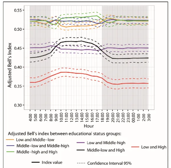
Adjusted Bell’s indices was plotted in Figure 5 to illustrate how co-presence of members of various social groups in the same district vary around the clock.
Figure 5: Adjusted Bell’s indices between the four educational status groups around the clock
Source: EGT, 2010 (STIF-OMNIL-DRIEA).
Values of the adjusted Bell’s index emphasize one major (though expected) social mechanism: the probabilities of co-presence are found to be systematically lower as the groups are socially distant. Or, to put it another way, co-presence is least frequent – at any time of the day or night - between highest social group and lowest social group and most frequent between socially close groups.
Globally, co-presence probabilities do not vary strongly across time except with and for the higher social class. Actually differences between night-time and day-time values (especially in the morning) are statistically significant for the pairs “high low group” and “high group-middle low group”. Daily mobility favors co-presence more especially with upper class members because of their own mobility of upper class members, but also because of the
17 mobility of other social class members towards districts with large concentration of higher class residences.
While probabilities of co-presence are found to be higher at night between “Low and Middle-High groups” than between “Middle-Low and Middle-High groups”, the contrary is observed during the day: members from “Middle-Low and High groups” have higher probability to be during the day in the same district than “Low and Middle-High groups.
We can interestingly notice in Figure 5 that it is during evening period (21:00) that there are the lowest probabilities for individuals from lower educational status and from middle-low educational status to share the same district as individuals from highest social groups.
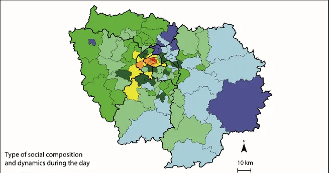
4.4 Social composition of districts in the Paris region around the clock
From the principal component analysis, four components are found to gather 79 per cent of the variance of the initial 13 indicators. Hierarchical clustering performed on these four components led to a division into eight district clusters, as mapped in Figure 6. Cluster profiles are summarized in Appendix A. For every cluster, average scholarship duration, diversity in educational status, and evolution of population size were calculated hourly using as an example the district which was closest to the cluster’s center of gravity (Figure 7).
During both the day and the night, the educational profile of the population present in the western inner Paris and adjacent western municipalities is very high, which underlines the well-known social composition of the Paris region from residential-based data. Central arrondissements (Ier, IIème, IIIème, IVème, VIIIème, IXème arrondissements; cluster 3) are found to experience the most drastic population growth (+150% between night-time and day-time, Appendix A) and social heterogenization during working hours. These districts are specifically very socially selective at evening, when recreational activities are from far the most frequent activities carried out, with the lowest educational mixity (entropy values) during this period: this may reflect the late departure of highly skilled workers, but also that these districts are places where the higher class socializes. Arrondissements of southwest Paris (Vème, VIème, XIVème, XVème, XXVIème arrondissements and Saint-Cloud; cluster 2) are the most homogeneous urban areas at night in the whole Paris region. With an increase in population during the day, social homogeneity decreases slightly but remains one of the highest. Districts located in inner Paris (Xème, XIème, XIIème, XIIIème, XVIIème, XVIIIème arrondissements; cluster 1) or in municipalities on the south-west periphery (e.g., Boulogne-Billancourt or Versailles) are upper class residential areas. Less socially homogeneous during the night than the previous two district clusters, they experience a slight heterogenization of social profile during the day. Districts concentrating populations with an intermediate level of education are the most heterogeneous areas during the night in the Paris region. In the first group of districts (e.g., XIXème arrondissement or Fontainebleau; cluster 4), the population is found to be more homogeneous and slightly less educated during the day than during the night, maybe in connection with a decrease in the working class population. In the second group of districts (e.g., XXème arrondissement, Saint-Germain-en-Laye or Rambouillet; cluster 5), mainly located in the westernmost periphery, a clear decrease in educational profile can be observed during the day as a consequence of a large population decrease (-31.5%; Appendix A). Over 24 hours, these districts constantly remain very mixed. The last group of middle class districts gathered peripheral districts close to inner Paris (e.g., Montreuil or Nanterre; cluster 6). These districts
18 are also very mixed. Values of entropy are the highest in the Paris region (Appendix A), in particular during the day. Moreover, population present during the day is found to be a bit more educated than population present during the night (cluster 6).
Districts concentrating the less educated population both during the day and the night are located on the northern and eastern peripheries. In the first group of districts (e.g., Villiers-le-Bel or Aulnay-sous-Bois; cluster 7), the population is found to be less numerous and less educated during the day than during the night. Moreover, these districts are the only ones to be more homogeneous by day than by night, maybe because of the departure of more educated residents to work places. In contrast, in the second group of districts (e.g., Tremblay-en-France or Saint-Denis; cluster 8), the population is found to be more educated during the day than during the night, and then more mixed. This variation occurs with an increase in population, more educated than the resident population and coming to these areas to work - for instance in the international activity area next to Charles-de-Gaulle airport for Tremblay-en-France, or in the Plaine Saint-Denis (tertiary, industrial, and academic activities) for Saint-Denis.
Figure 6: District classification in the Paris region according to their social composition around the clock
19
Figure 7: Average scholarship duration, diversity in educational status, and population size around the clock for eight districts in the Paris region
Source: EGT, 2010 (STIF-OMNIL-DRIEA).
20
5 Concluding discussion
5.1 Methodological points
Some methodological aspects need to be discussed. The main one deals with districts’ sizes. With a median size of 14 km², these spatial units are too large to be consistent with the experienced neighborhood. Previous studies carried out in the Paris region showed that perceived neighborhoods have a median size of 0.22 km², with a large variety according to population income and municipality population size (Vallée et al., 2014; Vallée et al., 2016). In addition, we can observe some important variability between the 109 districts’ sizes (from 3 to 1,326 km²), even if their resident population sizes are approximately similar (around 100,000 inhabitants). Though considering areas as small as possible is not necessarily better when exploring neighborhood effects and people’s neighborhood experience (Vallée et al., 2014), it would have been seductive to explore variation in social composition over 24 hours using smaller units than districts. However, it would have been too risky since EGT survey was not designed to produce valid estimations in smaller units that districts. To be able to use smaller spatial units when investigating social segregation around the clock, it may be tempting to use an exhaustive population database such as a census or a very large database (such as mobile phone data). However, these databases have other major disadvantages: a census does not give information about respondents’ daily trips (focusing often only on their commuting practices) and mobile phone data do not give information about respondents’ social profile for reasons of confidentiality. As things stand at present, a large travel survey provides an appropriate balance to explore changes in social composition over 24 hours. The limitation of data sources in exploring segregation on a continuum of place versus people-based measures is a constant problem exposed in the literature (Farber et al., 2015).
Two other points also need to be mentioned. Firstly, we only used daily trips on weekdays (Monday-Friday) to explore social segregation around the clock. It would also be interesting to explore what happens at the weekend. Unfortunately, the sample of daily trips at weekends was too small in the EGT survey. Secondly, the EGT database was limited to inhabitants living in the Paris region. Populations residing outside the region but visiting the region during the day (long-distance workers, tourists, consumers, etc.) have not been taken into consideration, even though their daily mobility may be very specific (e.g., for foreign tourists; Olteanu-Raimond et al., 2012). Moreover, some places, such as touristic, business, or commercial centralities, may attract very specific populations at a national and international scale (e.g., for popular commercial centrality; Chabrol, 2011) and their social composition around the clock may then largely differ in resulting maps, depending on whether or not inhabitants living outside the Paris region are considered.
5.2 Synthesis of findings
Four main findings emerge from our original analysis of segregation around the clock in the Paris region.
First of all, the extent of social segregation in the Paris region was found to be weaker during the day than during the night. This result is consistent with the study by Silm and Ahas (2014) on spatiotemporal variations of (ethnic) segregation in Tallinn (Estonia) and with findings comparing residential segregation and workplace segregation (ethnic again) in Los Angeles
21 (Ellis et al., 2004). By analogy to Silm and Ahas’ study who wrote that "ethnic groups are distributed much more evenly in the city during daytime, on workdays, and in the summer than is indicated by the places of residence of the ethnic groups", we can affirm that social groups are also more evenly distributed in the Paris region during daytime than during the night and that the probability of co-presence of distinct social groups is higher during the day. A study on ethnic segregation in Tel Aviv among African workers underlined their extreme isolation when focusing on social interactions regardless of their level of exposure to non-Africans in their frequented neighborhoods (Schnell and Yoav, 2001). Let us then recall that our results do not signify more social interactions between social groups during the day and could be challenged by studies focusing on real interactions between people. In our study, working is the main activity explaining this mixing of social groups, whereas leisure activities during the day seem to be more socially compartmentalized. In that sense, segregation at the weekend would have been interesting to study, as weekend trips are less dependent on mobility constraints such as commuting.
Secondly, when exploring segregation around the clock, we observe that social groups who were the most segregated during the night were also those who were the most segregated during the day. The upper class was the most segregated group, followed by the lower class. Upper class members are those who put more spatial distance with other social groups’ members during at night, although it changes during day-time. Elites have been qualified in residential-based data as “beneficiaries and drivers of residential segregation in Paris” (Préteceille, 2006) and this assertion can then easily be extended when adopting an activity-based approach. Findings also underline that it is the upper class whose social environment evolves the most strongly during day-time, as some of them move to less favored neighborhoods to work and, above all, as they live in the areas the most dense in jobs, during the day-time they see a more diverse population coming for work. Indeed, as it was shown in earlier studies, spatial mismatch is much lower for executives than for workers in the Paris region (Wenglenski, 2004).
Thirdly, the present paper underlines the major role played by employment in social diversity dynamics during the day-time. Working (or studying) is indeed the main motivation for leaving the place of residence during a weekday. Moreover, areas dense in jobs experience large social heterogenization during day-time whether they are residence places of the upper class or the lower class (Appendix A). Areas poorly supplied by jobs become poorer during the day, as less favored individuals stay in their neighborhoods during the day-time and the most educated or favored people leave the neighborhood to go to work in other parts of the city. However, it would be too simplistic to explain variations over 24 hours in district’s social composition only by home-work trips. Evening activities (mainly recreational, see Figure 1) lead also some change in districts social composition. When comparing evening and night periods (Additional table), important changes in social level, social mixity and population number can be underlined, notably for central Paris arrondissements (cluster 3 in Figures 6 and 7). Moreover, the lowest probabilities for more socially deprived people to share the same district as less socially deprived people occurr during the evening period (Figure 5).
Crossing residential and daily dynamics reproduces more faithfully the social characteristics of populations present in commercial nodes or clusters of workplaces, for instance. For the non-mobile population, living in a poor neighborhood which is impoverished during the day may
22 not have the same effect as living in a poor neighborhood that attracts a more affluent population during the day.
Lastly, the present paper highlights deep social variations in districts’ social composition over 24 hours. Districts may have similar social composition during the night, but their social composition can evolve in a very different way during the day-time. In some peripheral districts, we observe a strong decrease in population’s social level during day-time because of departure of the less socially deprived people in other parts of the city and the retention of most socially deprived people. This pauperization process can be discussed making an analogy with the filtering process notion more commonly used in link with residential mobility (Hoyt, 1939). “Residential” filtering process has been used to explain the decline in socioeconomic status of neighborhood’s residential population through the deterioration in housing stock, parks, streets, schools, and retail businesses over time and the households’ residential mobility from and to this neighborhood (departure of the wealthiest households to more attractive neighborhoods, maintenance of the most modest households, and installation of modest households in the neighborhood). Actually these processes explaining over-concentration of deprived population in some areas “at night-time” may be coupled with processes explaining concentration of deprived population in the same areas “at day-time”: departure of the most favored people to areas providing more local (work, leisure etc.) resources and retention of disadvantaged people. The most critical areas where public actors have to implement interventions actions could then be those where residential and daily filtering processes occur.
5.3 Conclusion
The present paper urges then a more general consideration of daily mobility as both reflecting and driving social and spatial division in cities. Such an approach may help scholars to consider dynamically neighborhood attributes and neighborhood effects. Crossing residential and daily dynamics reproduces indeed more faithfully the social characteristics of populations present in commercial nodes or clusters of workplaces, for instance. For the non-mobile population, living in a poor neighborhood which is impoverished during the day may not have the same effect as living in a poor neighborhood that attracts a more affluent population during the day. Taking daily mobility into account may also help public and municipal actors to implement some interventions in areas with a high concentration of specific social groups around the clock and to reduce more effectively social inequalities within the metropolitan area.
Acknowledgements
We are grateful to STIF, OMNIL, DRIEA and ADISP-CMH who have made EGT data available through « Réseau Quetelet ». We also thank the three reviewers for their valuable comments and suggestions regarding our manuscript.
Funding sources
RelatHealth project (http://relathealth.parisgeo.cnrs.fr) was supported by Université Sorbonne
23
Appendix A
Summary of districts’ profiles in the Paris region for every eight clusters issued from classification Cluster 1 Cluster 2 Cluster 3 Cluster 4 Cluster 5 Cluster 6 Cluster 7 Cluster 8 Variables from curves of evolution per hour Average social level** 13.4 14.1 14.0 11.7 11.9 12.3 10.8 10.4 Average entropy*** 0.93 0.84 0.87 0.96 0.96 0.97 0.92 0.90 Range of the average
social level (% of
average) 4.8% 6.1% 7.3% 4.1% 7.3% 4.0% 5.6% 6.9% Range of the average
entropy (% of average) 6.2% 17.6% 15.7% 3.7% 4.3% 2.5% 5.3% 8.6% Variables computed upon time slots*
Social level rate of change, night/day-time -3.0% -3.9% -3.5% -0.7% -4.8% 1.4% -2.3% 4.0% Entropy rate of change, night/day-time 4.4% 14.0% 8.6% 1.0% 0.1% 0.3% -0.5% 6.1% Population rate of change, night/day-time -1.5% 9.2% 150.4% -16.3% -31.5% 8.1% -22.7% -7.6% Social level rate of
change, day-time/evening 2.1% 3.1% 4.7% 0.0% 3.7% -1.5% 1.3% -3.9% Entropy rate of change, day-time/evening -2.5% -8.6% -10.0% -1.1% -0.2% -0.2% -0.4% -5.3% Population rate of change, day-time/evening -1.6% -7.5% -41.7% 12.9% 34.9% -8.9% 24.2% 5.7% Social level rate of
change, evening/night 1.0% 1.0% -1.0% 0.7% 1.3% 0.2% 1.1% 0.1% Entropy rate of change, evening/night -1.7% -3.9% 2.3% 0.1% 0.2% -0.1% 0.9% -0.4% Population rate of change, evening/night 5.5% 4.0% -30.5% 6.7% 9.3% 5.3% 5.3% 4.1% Illustrative contextual variables Employment**** density median (/km2) 13,590 15,344 39,157 669 433 4,155 663 1,145
Notes: * Time slots: day-time = 8:00–18:00; evening = 18:00–23:00; night = 23:00–8:00. Statistics computed by weighting population in the district by the presence duration within the time slot.
** Social level: mean of the scholarship duration of people in the district. *** Entropy: entropy measure computed on the four groups of educational status.
**** Number of jobs in the district (from the French census) divided by the area of the district. Sources: EGT, 2010 (STIF-OMNIL-DRIEA). INSEE, 2013.
References
Abrahamson, M., Sigelman, L., 1987. Occupational sex segregation in metropolitan areas.
American Sociological Review, 52(5), 588–597.
Amar, G., 1993. Pour une écologie urbaine des transports. Annales de la Recherche Urbaine, n°59–60, 140–151.
24 Åslund, O., Skans, O. N., 2010. Will I see you at work? Ethnic workplace segregation in Sweden, 1985–2002. Industrial & Labor Relations Review, 63(3), 471–493.
Authier, J.-Y., 1993. La vie des lieux. Un quartier du Vieux-Lyon au fil du temps. Lyon: Presses Universitaires de Lyon.
Bell, W., 1954. A probability model for the measurement of ecological segregation. American
Sociological Review, 32, 357–364.
Billari, F.C., 2001. The analysis of early life courses: complex descriptions of the transition to adulthood. Journal of Population Research, 18(2), 119–142.
Borsdorf, A., Hidalgo, R., 2009. The fragmented city. The Urban Reinventors Online Journal, 3(9), 1–18.
Buliung, R. N., Matthew J. R., Tarmo, Remmel K., 2008. Exploring spatial variety in patterns of activity-travel behaviour: initial results from the Toronto Travel-Activity Panel Survey (TTAPS). Transportation, 35, 697–722.
Carlstein, T., Parkes, D., Thrift, N. (Eds), 1978. Human Activity and Time Geography. London: Edward Arnold Publishers.
Chabrol, M., 2011. De nouvelles formes de gentrification? Dynamiques résidentielles et
commerciales à Château-Rouge (Paris). PHD Thesis, Poitiers: Université de Poitiers.
Chamboredon, J.-C., Lemaire, M., 1970. Proximité spatiale et distance sociale. Les grands ensembles et leur peuplement. Revue Française de Sociologie, 11(1), 3–33.
Chapin, F.S, Stewart, P.H., [1953] 1964. Population densities around the clock. In: Mayer, H.M., Kohn, C.F. (Eds), Readings in Urban Geography. Chicago: The University of Chicago Press, pp. 180–182.
Chenu, A., 2000. Le repérage de la situation sociale. In : Leclerc A. et al. (Eds). Les inégalités
sociales de santé. Paris : La Découverte, 93–107.
Cliff, A. D., Ord, J. K., 1981. Spatial processes : Models & Applications. London : Pion. Cools, M., Moons, E., Wets, G., 2010. Assessing the quality of origin-destination matrices derived from activity travel surveys. Transportation Research Record, 2183, 49–59.
Cortese, C.F., Falk, R.F., Cohen, J.K., 1976. Further considerations on the methodological analysis of segregation indices. American Sociological Review, 41(4), 630–637.
Cowgill, D.O., Cowgill, M.S., 1951. An index of segregation based on block statistics.
American Sociological Review, 16(6), 825–831.
Duncan, O.D., Duncan, B., 1955. Residential distribution and occupational stratification.
American Journal of Sociology, 60(5), 493–503.
Ellis, M., Wright, R., Parks, V., 2004. Work together, live apart? Geographies of racial and ethnic segregation at home and at work. Annals of the Association of American Geographers, 94(3), 620–637.
25 Farber, S., O’Kelly, M., Miller, H.J., Neutens, T., 2015. Measuring segregation using patterns of daily travel behavior: a social interaction based model of exposure. Journal of Transport
Geography, 49, 26–38.
Foley, D.L., 1952. The daily movement of population into Central Business Districts. American
Sociological Review, 17(5), 538–543.
Foley, D.L., 1954. Urban day-time population. Social Forces, 32(4), 323–330.
Girault, F., Bussi, M., 2001. Les organisations spatiales de la ségrégation urbaine: l'exemple des comportements électoraux. L’Espace Géographique, 30(2), 152–164.
Goodchild, M.F., Janelle, D.G., 1984. The city around the clock: space-time patterns of urban ecological structure. Environment and Planning A, 16, 807–820.
Grannis, R., 2002. Discussion: segregation indices and their functional inputs. Sociological
Methodology, 32, 69–84.
Hellerstein, J.K., Neumark, D., 2008. Workplace segregation in the United States: Race, ethnicity, and skill. The Review of Economics and Statistics, MIT Press, 90(3), 459–477, 04. Hornseth, R.A., 1947. A note on ‘The measurement of ecological segregation’ by Julius Jahn, Calvin F. Schmid, and Clarence Schrag. American Sociological Review, 12(5), 603–604. Hoyt, H., 1939. The Structure Growth of Residential Neighborhoods in American Cities. Washington: Federal Housing Administration.
Jahn, J.A., 1950. The measurement of ecological segregation: derivation of an index based on the criterion of reproducibility. American Sociological Review, 15(1), 100–104.
Jahn, J.A., Schmid, C.F., Schrag, C., 1947. The measurement of ecological segregation.
American Sociological Review, 12(3), 293–303.
Jones, P., Clarke, M., 1988. The significance and measurement of variability in travel behavior.
Transportation, 15, 65–87.
Krivo, L. J., Washington, H. M., Peterson, R. D., Browning, C. R., Calder, C. A., Kwan, M. P., 2013. Social isolation of disadvantage and advantage: The reproduction of inequality in urban space. Social forces, 92(1), 141–164.
Kwan, M.-P., 2009. From place-based to people-based exposure measures. Social Science and
Medicine, 69, 1311–1313.
Lee, J. Y., Kwan, M. P., 2011. visualisation of socio‐spatial isolation based on human activity patterns and social networks in space‐time. Tijdschrift voor economische en sociale geografie, 102(4), 468–485.
Massey, D.S., 1978. On the measurement of segregation as a random variable. American
Sociological Review, 43(4), 587–590.
Massey, D.S., Denton, N.A., 1988. The dimensions of residential segregation. Social Forces, 67(2), 281–315.
26 Massot, M.-H., Zaffran, J., 2007. Auto-mobilité urbaine des adolescents franciliens. Espace
Populations Sociétés, 2007(2–3), 227–241.
May, N., Veltz, P., Landrieu, J., Spector, T., 1998. La Ville Éclatée. Aigues: Éditions de l'Aube. Musterd, S., 2006. Segregation, urban space and the resurgent city. Urban Studies, 43(8), 1325– 1340.
Olteanu-Raimond, A.-M., Couronné, T., Fen-Chong, J., Smoreda, Z., 2012. Le Paris des visiteurs étrangers, qu'en disent les téléphones mobiles? Inférence des pratiques spatiales et fréquentations des sites touristiques en Ile-de-France. Revue Internationale de Géomatique, 22(3), 413–437.
Orfeuil, J.-P., 2002. Etat des lieux des recherches sur la mobilité quotidienne en France. In Lévy, J.-P., Dureau, F. (Eds), L’Accès à la Ville. Les mobilités spatiales en question. Paris: L’Harmattan, 65–98.
Palmer, J. R., 2013. Activity-space Segregation: Understanding social divisions in space and
time. PHD Thesis, Princeton: Princeton University.
Park, R.E., 1925. The city: suggestions for the investigation of human behavior in the urban environment. In: Park, R.E., Burgess, E.W. (Eds). The City. Chicago: University of Chicago Press, 1–46.
Pas, E. I., 1987. Intrapersonal variability and model goodness-of-fit. Transportation Research Part A, 21(6), 431–438.
Pinçon, M., Pinçon-Charlot, M., 2007. Les Ghettos du Gotha : comment la bourgeoisie défend
ses espaces. Paris: Le Seuil.
Préteceille, E., 2006. La ségrégation sociale a-t-elle augmenté? Sociétés Contemporaines, 2, 69–93.
R Core Team, 2016. R: A Language and Environment for Statistical Computing. Vienna (Austria): R Foundation for Statistical Computing.
Reardon, S.F., Firebaugh, G., 2002. Measures of multigroup segregation. Sociological
Methodology, 32(1), 33–67.
Reardon, S.F., O’Sullivan, D., 2004. Measures of spatial segregation. Sociological
Methodology, 34, 121–162.
Schnell, I., Yoav, B., 2001. The sociospatial isolation of agents in everyday life spaces as an aspect of segregation. Annals of the Association of American Geographers, 91, 622–636. Silm, S., Ahas, R., 2014. The temporal variation of ethnic segregation in a city: evidence from a mobile phone use dataset. Social Science Research, 47, 30–43.
Small, M.L., 2007. Racial differences in networks: do neighborhood conditions matter? Social
Science Quarterly, 88(2), 320–343.
27 Taeuber, K.E., Taeuber, A.F., 1976. A practitioner's perspective on the index of dissimilarity.
American Sociological Review, 41(5), 884–889.
Urry, J., 2002. Mobility and proximity. Sociology, 36(2), 255–274.
Vallée, J., Le Roux, G., Chaix, B., Kestens, Y., Chauvin, P., 2015. The ‘constant size neighbourhood trap’ in accessibility and health studies. Urban Studies, 52(2), 338–357.
Vallée, J., Le Roux, G., Chauvin, P., 2016. Quartiers et effets de quartier. Analyse de la variabilité de la taille des quartiers perçus dans l’agglomération parisienne. Annales de
Géographie, 2, 119–142.
Wenglenski, S., 2004. Une mesure des disparités sociales d'accessibilité au marché de l'emploi en Ile-de-France. Revue d’Économie Régionale & Urbaine, 4, 539–550.
White, M.J., 1983. The measurement of spatial segregation. American Journal of Sociology, 88(5), 1008–1018.
White, M.J., 1986. Segregation and diversity measures in population distribution. Population
index, 52(2), 198-221.
Wickham, H., 2009. ggplot2: Elegant Graphics for Data Analysis. New York: Springer-Verlag. Williams, J.J., 1948. Another commentary on so-called segregation indices. American
Sociological Review, 13(3), 298–303.
Wong, D.W., 2005. Formulating a general spatial segregation measure. The Professional
Geographer, 57(2), 285–294.
Wong, W.S., Shaw, S.L., 2011. Measuring segregation: an activity space approach. Journal of