HAL Id: hal-02872350
https://hal.archives-ouvertes.fr/hal-02872350
Submitted on 17 Jun 2020
HAL is a multi-disciplinary open access
archive for the deposit and dissemination of
sci-entific research documents, whether they are
pub-lished or not. The documents may come from
teaching and research institutions in France or
abroad, or from public or private research centers.
L’archive ouverte pluridisciplinaire HAL, est
destinée au dépôt et à la diffusion de documents
scientifiques de niveau recherche, publiés ou non,
émanant des établissements d’enseignement et de
recherche français ou étrangers, des laboratoires
publics ou privés.
Wet deposition in a global size-dependent aerosol
transport model
W. Guelle, Yves Balkanski, J. Dibb, M Schulz, F. Dulac
To cite this version:
W. Guelle, Yves Balkanski, J. Dibb, M Schulz, F. Dulac. Wet deposition in a global size-dependent
aerosol transport model: 2. Influence of the scavenging scheme on 210Pb vertical profiles, surface
con-centrations, and deposition. Journal of Geophysical Research: Atmospheres, American Geophysical
Union, 1998, 103 (D22), pp.875 - 903. �10.1029/98JD01826�. �hal-02872350�
JOURNAL OF GEOPHYSICAL RESEARCH, VOL. 103, NO. D22, PAGES 28,875-28,891, NOVEMBER 27, 1998
Wet deposition in a global size-dependent aerosol
transport model
2. Influence of the scavenging scheme on
vertical
profiles, surface concentrations, and deposition
W. Guelle, 1 y. j. Balkanski,
1 j. E. Dibb, 2 M. Schulz,
3 and F. Dulac •
Abstract. The main atmospheric sink for submicron aerosols is wet removal.
Lead 210, the radioactive
decay product of 222Rn,
attaches
immediately after being
formed to submicron particles. Here we compare the effects of three different
wet-scavenging
schemes
used in global aerosol
simulations
on the 2•øPb aerosol
distribution using an off-line, size-resolved, global atmospheric transport model. We highlight the merits and shortcomings of each scavenging scheme at reproducing available measurements, which include concentrations in surface air and deposition, as well as vertical profiles observed over North America and western and central North Pacific. We show that model-measurement comparison of total deposition does not allow to distinguish between scavenging schemes because compensation effects can hide the differences in their respective scavenging efficiencies. Differences in scavenging parameterization affect the aerosol vertical distribution to a much greater extent than the surface concentration. Zonally averaged concentrations at different altitudes derived from the model vary by more than a factor of 3 according
to the scavenging
formulation, and only one scheme
enables us to reproduce reliably
the individual profiles observed. This study shows that ground measurements alone are insufficient to validate a global aerosol transport model.
1. Introduction
Very little has been done to evaluate tropospheric aerosol vertical distribution predicted from models against actual measurements. This represents a clear gap in our ability to adequately represent aerosol mass and number concentrations, to assess their direct radia- tive effect, and to estimate the heterogeneous reactions that take place at their surfaces. A description of the processes that affect aerosol number concentration ne- cessitates a good representation of the fate of the aerosol
in and below clouds.
Boucher [1995, p. 87] highlighted the differences that
arise in sulfate distributions between the models MO-
GUNTIA and IMAGE. Not only are the amplitude of the resulting radiative forcings different, but the tim-
1Laboratoire des Sciences du Climat et de l'Environne-
ment, Laboratoire mixte Commissariat k l'Energie Atom-
ique/Centre National de la Recherche Scientifique, Gif-sur-
Yvette, France.
2Institute for the Study of Earth, Oceans, and Space, Uni- versity of New Hampshire, Durham, NH.
3Institut fiir Anorganische und Angewandte Chemie, Uni-
versit/it Hamburg, Hamburg, Germany.
Copyright 1998 by the American Geophysical Union.
Paper number 98JD01826.
0148-0227 / 98 / 98 J D-01826509.00
ing of its northern hemisphere
maximum
is shifted by
nearly 3 months between the two models. Although these discrepancies are not only due to wet scavenging, the important role it has as the main sink for SO•- and an important pathway for SO2 removal makes it one
of the best candidates to explain these differences. We
are limited in terms of validation of the sulfate distri-
bution by the number of vertical profiles that have been measured for both sulfate and SO2 [Chin et al., 1996].
Heterogeneous chemistry has been documented to
take place on the surface of mineral aerosol [Maraane and Gotlieb, 1989] or sea-salt particles [Finlayson-Pitts, 1983]. The main limitations for assessing the impact
of these aerosols on tropospheric chemistry are twofold:
(1) a better knowledge of the sticking coefficients and (2) an evaluation of the surface of the aerosol available at any given time and place for these reactions to take place. We therefore need not only to represent mass correctly but also to compute aerosol size distribution. Until recently, global aerosol models computed only the aerosol mass. A step toward an accurate computation of
the aerosol surface and number concentration was done
either using 3 [Genlhon, 1992], 8 [Tegen and Lacis, 1996; Gong et al., 1997], 10 [Dentenet et al., 1996], or 20 size bins [Schulz et al., 1998], or using a spectral scheme that deals with modal parameters of size distribution [Schulz et al., 1998]. Since heterogeneous chemistry can occur
28,876 GUELLE ET AL.: INTERCOMPARISON OF AEROSOL WET-SCAVENGING SCHEMES
in the presence of SO• in the vicinity of aerosol surfaces, it is important to estimate both the three-dimensional (3-D) distributions of number concentrations and the
coincidence of sulfate and mineral aerosols in order tc
represent it.
For absorbing aerosols, the direct radiative effect strongly depends on their altitude. Tegen and Lacis
[1996] show that for a given optical thickness over a
given surface, mineral aerosol can have a positive or
2. Description of the Atmospheric Model
and of the Three Scavenging Schemes
2.1. Atmospheric Model
In this study we use the 3-D atmospheric model of tracer transport TM2 developed by M. Helmann at the Max-Planck-Institut fiir Meteorologie in Hamburg
[Heimann and Keeling, 1989; Helmann, 1995]. It is an
off-line model driven by the analyzed 12 hourly fields
negative
radiative
forcing
depending
on the altitude
of from
the European
Centre
For Medium-Range
Weather
the dust layer. It is therefore
necessary
to reproduce
Forecasting
(ECMWF).
This
version
of the model
has
a
well both
the horizontal
and the vertical
distribution
of 2.50
x 2.50
horizontal
resolution
IRamonet,
1994],
nine
the aerosols.
A discussion
of the vertical
distribution
of sigma
levels
extending
from
the ground
to 10 mbar,
and
mineral
aerosol
can
be found
in the work
of Duce
[1995]. is run with a i hour
time step. Horizontal
and verti-
This distribution consists over the oceans of structured
layers that extend above the marine boundary layer up to altitudes of 7 km. This pattern of aerosol distri-
bution is confirmed by lidar measurements [Iwasaka e!
al., 1983, 1988; Swap e! al., 1992; Chazette et al., 1997;
Dulac et al., 1997; Hamonou et al., 1997]. Vertical pro-
files of aerosols from biomass burning have been col-
lected by differential absorption lidar (DIAL) during the NASA Global Tropospheric Experiments/Amazon Boundary Layer Experiment (GTE/ABLE 2A)[Browell et al., 1988] which took place over the Amazon Basin in
July-August 1985. These vertical profiles showed con- siderable variations. The Transport and Atmospheric
Chemistry near the Equator-Atlantic (TRACE A) ex-
periment, which took place over the tropical South At- lantic in October 1992, showed enhanced aerosol load- ings as a result of biomass burning. The UV-DIAL pro- file allowed to identify the vertical extent of the aerosol
plumes over these regions [Anderson et al., 1996]. In a previous paper [Guelle et al., 1998] we presented
a i year simulation
of atmospheric
2•øPb
using
a global
aerosol transport model, and we extensively compared the model results to ground-based observations of con- centrations and deposition. Lead 210 is a tracer of submicronic size aerosol particles, which are principally
removed from the atmosphere by wet scavenging [Balka- nski et al., 1993]. In this paper we present a detailed
comparison of model simulations using our scheme and two other wet-scavenging schemes from the literature in order to focus on the influence of wet-removal parame- terization on aerosol distribution and deposition. Avail- able observations are used as a reference, with special emphasis on vertical profiles.
Section 2 describes how the three scavenging schemes, used to compute aerosol global distributions, differ. Section 3 highlights the differences in deposition and
2•øPb surface concentrations brought about by the dif-
ferent assumptions in scavenging. We then compare measured vertical profiles to those predicted by the model runs. Altitudinal measurements of •øPb are used in sensitivity studies to discuss the assumptions
made in the scheme presented by Guelle et al. [1998].
cal advection are computed using the slopes scheme of
Russell and Lerner [1981], with a slope limitation added to avoid negative concentrations [Schulz et al., 1998].
Subgrid-scale vertical exchange processes are performed
using the Louis [1979] formulation for turbulent vertical transport and a simplified version of the Tiedlke [1989] scheme to compute the mass fluxes in cumulus clouds.
The 3-D global simulations were conducted for the
year 1991 and part of the year 1994 (January through
March) when
the 2•øPb
vertical
profiles
were
measured.
The simulation of the whole year 1991, which is used for comparison with ground-based measurements, is
described by Guelle et al. [1998] for one of the wet-
scavenging schemes and has been repeated with the other two. Every simulation presented in this work has been initialized with an empty atmosphere and started 2 months before the period of study. For the profiles sampled during September-October 1991 and February- March 1994, the runs were started on July 1, 1991, and December 1, 1993, respectively, and lasted 4 months. These simulations have been computed the same way as for the whole year 1991, with some slight differences. First, since we did not dispose of ECMWF ground pre- cipitation fields for 1994, we have used the precipita-
tion fields from the National Centers for Environmental
Predictions/National Center for Atmospheric Research (NCEP/NCAR) reanalysis. While the 24 hour forecast precipitation fields from ECMWF for 1991 have a tem- poral resolution of 12 hours, the NCEP is 6 hourly. Both precipitation fields were regridded to the model resolu- tion. Since we compare the model results to profiles measured over a few hours, the model outputs of these two shorter simulations were sampled every 6 hours.
Lead 210 is produced from 222Rn. In the simulations
of fall 1991 and spring 1994, when we compare individ- ual vertical profiles, we used the daily concentrations of
222Rn
obtained
from a previous
simulation
IRamonet
and Monfray, 1996] to compute
the 2•øPb source
in
the model. The same run was repeated with the three scavenging schemes described below. Details about the
treatment of the size distribution can be found in the
GUELLE ET AL.' INTERCOMPARISON OF AEROSOL WET-SCAVENGING SCHEMES 28,877
sented, we have set the size distribution parameters of
ambient
aerosol
carrying
2•øPb to 0.4 tim for the mass
median diameter and 1.9 for the geometric standard de-
viation [Sanak et al., 1981; Bondietti et al., 1988]. The details of the 222Rn and 2•øPb simulations can be found in the work of Guelle et al. [1998], who compared ex- tensively the 2•øPb distribution obtained to available surface measurements of concentration and deposition. Here we focus on the description of the differences be- tween the three different scavenging schemes used.
2.2. Wet-Scavenging Schemes
The first scheme has been developed by Kasibhatla
et al. [1991] and has been adapted to the TM2 model by Rehfeld and Helmann [1995] to compute scavenging of radioactive tracers (hereinafter referred to as RH95). The second scheme, described by Walton et al. [1988] (hereinafter referred to as W88), has been used to scav- enge fire smoke [Ghan et al., 1988], nitrogen [Penner et al., 1991], carbonaceous aerosol [œiousse et al., 1996],
and 21øpb
aerosol
[Lee and Feichter, 1995]. Scheme
RH95 was chosen for its simple treatment of wet scav-
enging. Scheme W88 is widely used in global aerosol
simulations and has proven to give the best agreement with ground-based observations in a previous intercom-
parison paper of aerosol wet-scavenging schemes [Lee and Feichter, 1995]. Scheme 3 is the scheme used by
Balkanski
½t al. [1993]
for global
simulation
of 2•øpb
aerosol which has been expanded to deal with size-
distributed aerosols [Guelle et al., 1998]. It has been applied to mineral aerosol studies [Guell½, 1998] and is described by Guelle et al. [1998] (hereinafter referred
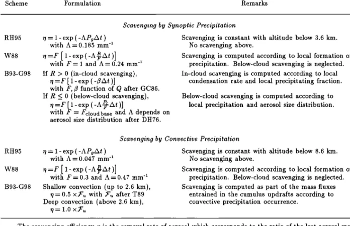
to as the B93-G98 scheme). Table 1 summarizes how the scavenging efficiencies are computed in these three
different schemes.
2.2.1. Scavenging by synoptic precipitation. The three schemes compute scavenging by synoptic pre- cipitation through first-order loss operators. In scheme RH95 the scavenging efficiency depends on the ground precipitation rate, which is equivalent to assume a con- stant scavenging ratio. Precipitating cloud heights are fixed to 3.6 km and do not allow the scavenging of the aerosol above. A buildup of the aerosol load occurs above 3.6 km altitude in regions where large-scale pre- cipitation dominates. Schemes W88 and B93-G98 are similar in their formulation of synoptic precipitation. They are both based on the work of Giorgi and Charnel-
des [1986], which accounts for the vertical distribution
of precipitation. The vertical profiles used for synoptic
precipitation
are those
from the GISS (Goddard
Insti-
tute for Space Studies) general
circulation
model [see
Guelle et al., 1998]. Only the B93-G98 scheme com-
putes separately below-cloud scavenging. While scheme RH95 does not separate below- and in-cloud scavenging, scheme W88 does not compute it at all, which is of lit- tle impact for global modeling of small particles such
as 2•øPb carriers
[Guelle e! al., 1998],
but could
intro-
duce a significant bias for large aerosols with diameters greater than i ttm. In the case of partial evaporation
the aerosol is not released but rather we assume that
the raindrop diameter is reduced. Part of the raindrops might undergo complete evaporation and release their nucleated particle in the atmosphere, although physi- cally a reduction in droplet diameter is more likely to occur. The sensitivity of the B93-G98 scheme to this assumption is discussed in section 3.
Table I shows that the formulations of the scavenging efficiency from schemes RH95 and W88 are similar since scavenging coefficients and the precipitating fractions are not much different. Therefore the only difference is
the rain amount taken into consideration in the scav-
enging at any height z. Scheme W88 uses the local pre- cipitation formation rate at height z, which represents only a fraction of the ground precipitation rate used by scheme RH95 at each altitude. Therefore these two scavenging schemes will lead to different aerosol vertical distributions, with more aerosol in scheme W88 below
3.6 km and more aerosol above 3.6 km in scheme RH95
since no scavenging occurs above that height.
Both scavenging schemes, W88 and B93-G98, take into consideration the vertical distribution of precipita- tion to scavenge aerosol. Scheme B93-G98 uses local precipitation formation rates to compute cloud water condensation rate, whereas W88 computes scavenging efficiency as a function of the formation of precipitation at height z. To compare schemes W88 and B93-G98, we computed the scavenging efficiencies of both schemes for different ground precipitation rates. The scaveng- ing efficiencies computed by B93-G98 are at least twice that calculated for scheme W88 at any height. We con- clude that scheme B93-G98 is more efficient at scaveng- ing aerosol by synoptic precipitation than the other two
schemes.
2.2.2. Scavenging by convective precipitation. Scheme B93-G98 computes aerosol scavenging in con- vective precipitation as part of the mass flux entrained
in convective cloud. The other two schemes use a first-
order loss coefficient with the same formulation as for
the synoptic precipitation. Scheme RH95 uses a con- stant scavenging coefficient up to 8.6 km. In the scheme W88, scavenging depends on the rate of formation of precipitation, but no scavenging occurs below cloud base. The vertical profiles needed in scheme W88 for convective precipitation are the ones derived from the
GISS model.
The main differences between the two schemes RH95
and W88 are as follows' in scheme W88, scavenging by convective precipitation is limited to 30% of the aerosol
mass in the grid box since F=0.3 (see Table 1). For
scheme RH95, all the aerosol mass in a given grid box can be scavenged, but the scavenging coefficient is 10 times less than for the W88 scheme. Supposing that
28,878 GUELLE ET AL.' INTERCOMPARISON OF AEROSOL WET-SCAVENGING SCHEMES
Table 1. Formulation of Scavenging Efficiency by Both Synoptic and Convective Precipitation for Three
Schemes
Scheme Formulation Remarks
RH95 r/= 1 -exp ( -APsAt )
with A=0.185 mm '•
W88
B93-G98
Scavenging by Synoptic Precipitation
r/-F [ 1- exp
(-A 7
with F= 1 and A= 0.24 mm -•
If R > 0 (in-cloud scavenging), r/=F[1-exp (-/?At)]
with F,/? function of Q after GC86.
If R _< 0 (below-cloud scavenging),
r/=F [ 1- exp
(-A • At )]
with F- Fclou dbase and A depends on
aerosol size distribution after DH76.
Scavenging is constant with altitude below 3.6 km. No scavenging above.
Scavenging is computed according to local formation of precipitation. Below-cloud scavenging is neglected. In-cloud scavenging is computed according to local
condensation rate and local precipitating fraction.
Below-cloud scavenging is computed according to local precipitation and aerosol size distribution.
RH95
W88
B93-G98
Scavenging by Convective Precipitation
r/= 1 -exp (-APsAt)
with A = 0.047 mm -•
,=F [ 1- exp
(-A•At)]
with F = 0.3 and A = 0.47 mm -•
Shallow convection (up to 2.6 km),
r/= 0.5 x.•, with .•, after T89
Deep convection (above 2.6 kin),
r/= 1.0 x.T'•,
Scavenging is constant with altitude below 8.6 km. No scavenging above.
Scavenging is computed according to local formation of precipitation. Below-cloud scavenging is neglected. Scavenging is computed as part of the mass fluxes
entrained in the cumulus updrafts according to convective precipitation occurrence.
The scavenging efficiency •/is the removal rate of aerosol which corresponds to the ratio of the lost aerosol mass within a time step At (hour) to the initial mass. It depends on a scavenging coefficient ,• (mm -1) or/? (s -1) and, according to the wet-scavenging scheme used, on the precipitating fraction of the grid box F, combined with either the ground precipitation rate Ps (mm h -1), or the local precipitation rate P• (mmh -1), or the local precipitation formation rate R (mmh -1), or the local condensation rate Q (kg m -3 s-1), or the aerosol mass fraction entrained
in the updrafts .•,. References given in this table are Dana and Hales [1976], Giorgi and Chameides [1986], Tiedtke [1989], and Balkanski et al. [1993].
the local precipitation rate is one tenth of the ground precipitation, the two scavenging schemes will compute
equal efficiencies
up to 8 mmh -•
According
to the
GISS vertical profiles, most of the convective precipita- tion is forming between 1.4 and 10.3 km altitude, cor- responding to four model layers in the TM2. Partition- ing the ground precipitation rate among these four lay- ers gives precipitation formation rates greater than the tenth of the ground precipitation rate in each of them, implying that scheme W88 is more efficient than scheme R}t95, except below i km where it does not compute
scavenging at all. Since mass fluxes (used by scheme B93-G98) and rainfall rates (used by the other two schemes) are not related in any simple way, we cannot
simply discuss the effects of the respective formulations of these two different types of wet-scavenging schemes. Respective results will be compared hereinafter.
3. Results and Discussion 3.1. Deposition
Table 2 presents the annual mean deposition fluxes
for 2•øPb as calculated from the three wet-scavenging
schemes. Both total deposition and deposition from
synoptic and convective precipitation are presented by averaging over each 300 latitudinal band. The differ- ences in surface deposition fluxes between the three
schemes
are small, ranging
from about 20 Bq m -2 yr -•
at high northern
latitudes
to less
than 10 Bq m -2 yr -•
in the tropics and southern hemisphere. Schemes RH95 and W88 agree closely, whereas the B93-G98 scheme
leads to higher values at high and midlatitudes and to
slightly lower values in the tropics.
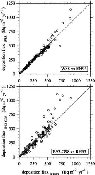
In order to determine whether deposition measure- ments could allow to distinguish between these schemes, we have compared the annual total deposition fluxes simulated by the three schemes at the 147 sampling
stations presented by Guelle e! al. [1998]. Results are
shown in Figure 1. We clearly see that the deposition fluxes predicted by schemes RH95 and W88 are almost equal and very similar to those simulated by scheme B93-G98. The only noticeable differences between the
three schemes (highest values in Figure 1) occur at sta-
tions experiencing strong convective precipitation as-
sociated with the monsoon regime (India and Japan). These conclusions agree with Lee and Feichter [1995].
They found very similar yearly mean biases between
GUELLE ET AL.: INTERCOMPARISON OF AEROSOL WET-SCAVENGING SCHEMES 28,879
Table 2. Zonal Averages
of Annual 2•øPb
Deposition
by 300 Wide Latitudinal Band for Each
of the Three Schemes and for Each Deposition Type
Deposition, Bq m -2 yr -•
Scheme RH95 Scheme W88 Scheme B93-G98
Latitude Conv. • Syno. b Total c Conv. Syno. Total Conv. Syno. Total
90øN-60øN 11 66 96 19 44 89 15 78 108 60øN-30øN 47 65 133 67 45 136 50 75 144 30øN-0øN 75 5 97 78 3 98 60 10 87 0øS-30øS 45 4 58 46 3 58 34 10 53 30øS-60øS 13 14 29 15 11 28 10 23 34 60øS-90øS I 6 7 I 5 8 I 8 9 Global 42 21 75 47 15 75 35 28 75
Conv., convective; Syno., synoptic. •Flux due to convective precipitation.
b Flux due to synoptic precipitation.
cThe difference between the total deposition and the sum of the two different wet deposition fluxes gives the turbulent dry deposition contribution.
1250 ,,,,,,,,, _ 1000
•
500;
o o
250 0 250 500 7 _ _ o o•000
o o
0 0
• ?•0
o ø
o
• oo • 0 = •00 • - - o odepositionflux
RH95
(Bqrn
-2 yr
-1
)
Figure 1. Comparison between the annual total de-
position
flux (Bqm-2yr -•) simulated
by the three
schemes at the 147 sampling stations presented by
Gu½ll½ ½t al. [1998].
wet-scavenging schemes at 122 stations, with differences ranging from 6.0 to 9.6%.
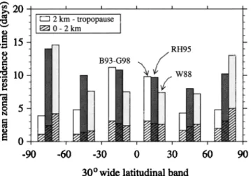
Figure 2 compares
the residence
time of 2•øPb for
each 300 latitudinal band and the 2•øPb content of the free troposphere and of the boundary layer. We define the free tropospheric residence time as the ratio of the total free tropospheric content divided by the total de- position at the surface. In scheme W88 the residence times are the same for both the tropics and the mid- latitudes in both hemispheres. Looking at the tropics where convective precipitation dominates and at high latitudes where most precipitation is synoptic, it is clear that the most efficient scheme at scavenging in the trop- ics is W88, whereas B93-G98 is the most efficient at high latitudes. Table 2 and Figure 2 show that different par- titionings of the three removal processes at midlatitudes can lead to the same residence times. For example, at northern midlatitudes, schemes RH95 and W88 both have nearly the same total deposition and residence times but with very different contributions from convec- tive and synoptic precipitations. It is noteworthy that a negative feedback operated in the deposition: weaker scavenging will increase aerosol tropospheric concentra- tion, which in turn increases the total deposition. Over long periods this feedback evens out differences in to- tal deposition fluxes between the two schemes. Given
all the above remarks and the small differences in total
deposition seen in Figure 1, we conclude that a compar- ison between simulated and observed deposition alone is of limited use to assess the accuracy of a scavenging
scheme.
3.2. Surface and Vertically Integrated
Concentrations
Figure 3 displays the global distribution of the annual
mean tropospheric 2•øpb concentrations. In Table 3 we
28,880 GUELLE ET AL.: INTERCOMPARISON OF AEROSOL WET-SCAVENGING SCHEMES I I
lEE3
•10-2•2
km
- tropopause
I
RH95 :.i B93-G98 i i i i -60 -30 0 30 W88 0 -90 90 i30 ø wide latitudinal band
Figure 2. Zonal averages
of mean annual 21øpb
res-
idence time (days) from 0 to 2 km (hatched bar) and from 2 km to the tropopause (as defined in Table 3) (clear bar) by a 30 ø wide latitudinal band for the schemes RH95 (dark grey), W88 (light grey), and B93- G98 (white).
We have compared the predicted monthly averaged
concentrations in surface air from each of the three
simulations with those observed at several stations. It
is important to note that we only present results at the stations, among the 35 presented by Guelle et al.
[1998], for which there are the most significant differ- ences between the monthly concentrations simulated with the three schemes. Results are shown in Fig-
ures 4a-4c. We grouped the high latitudes together
in Figures 4a (northern hemisphere) and 4b (southern hemisphere) to focus on the treatment of synoptic pre- cipitation. The scheme W88 overestimates the observed concentrations by a factor of 2, whereas the other two schemes predict concentrations in much closer agree-
ment with the observed values. If we consider annual
concentrations in surface air at the 59 stations presented by Guelle et ai. [1998] located poleward of 40 ø lat-
itude, the mean bias against observed values is-4% with scheme B93-G98, but +10% with scheme RH95
and +32% with scheme W88 (bias(%)=100 x (cOnCmoa-
trations simulated with the three schemes for each 30 ø
wide latitudinal band (the troposphere is defined from
the ground to 16, 10, and 9 km for latitudinal bands 0 ø-
30 ø , 300-60 ø , and 600-90 ø , respectively). Different scav-
enging schemes lead to large differences in either tro- pospheric or surface concentrations compared to much
smaller differences in surface deposition (see Table 2).
At high latitudes the schemes RH95 and W88 predict concentrations greater by more than a factor of 2 com- pared to B93-G98. Moreover, whereas schemes B93-
G98 and RH95 lead to similar surface concentrations at
northern and southern midlatitudes, scheme W88 leads to larger concentrations. Close agreement among the three schemes is found in the tropics. We also note that the aerosol atmospheric loading in scheme RH95 is greater than the other two schemes for all latitudinal bands, due to higher upper tropospheric concentrations. This buildup yields to an elevated mean annual tropo-
spheric residence time (9.5 days compared to 7.2 days estimated by Turekian et al. [1977] and 6.5 days by Lambert et ai. [1982]). With the other two schemes
(B93-G98
and W88), 21øpb
has a residence
time of 7.2
and 7.8 days.
Surface level concentrations (Table 3) differ mostly
at high latitudes. Although the three schemes lead to similar surface concentrations in the tropics, scheme W88 yields higher concentrations than the other two deposition schemes at middle and high latitudes. In
all three cases
the vertical gradient
of 21øpb
shows
in-
creased concentrations with altitude between 60øS and
90øS because of the remote location of sources at these
latitudes. It is noticeable that on a global average, tropospheric concentration is about 35% larger with
scheme RH95 than with the other two schemes due to
the limited height where scavenging takes effect. At high southern latitudes, scheme W88 predicts surface concentrations 20% higher than the other two schemes.
-180 410 4,0 0 60 1.7.0 180 ß . •..• ... .:."...:. :::::::::::::::::::::::::::::::::::::::::: ... ::..•;•::,.-:•:• :•;:•.: .• ... • '• ': :. •:" ::;Z :.•.. :;.•:::•..:>--,• •.. •.•:• ... ••••••••••2::•. .... :*•::'•:':::•::'•:•:'•'::':: ... •.::•...,.?•A::" '.' •. •' "*% :-: • :-- •i .: •..• 1 *. ß -:-. - ... ::" ."' :-.:::.:-•-.: •:.:.:;...: •.. ... :-•: .•:.- -' ... .::'---':'-'::•:>'?• .• -. s,. .... ---... -.- .:-.. -- .- -'I.• -'I.• • 0 • 1.• • '•.,.: *. :: ... '::' "t t ::::'... ':-•"'•..; ."•'*.:,:2":--:. ß * * •i • •.': ... '.; ',Z}.•l I . ..:.... w:.;::;,;:.•..,...•½.v.*.**•,..?-?,&2*•:,•½.•:,.,: .':?:c•;.•,: ',.c•-. • .'---.?½:;; ,:•:?;.,-/' '• C,: •:•.•.•:s.*:•:?•;;;;:/•;•:•*:•?.•.•.*•::::•*•..•.•`•.•••••••••:•:•. .... '•-*' .... • •'••••••••••••:S...•::'"":::*:.:X?*'•Ca ß
===================================
.:..:..
w'ss-;
-.• 4• • 0 • • • ... • ?aXf**•::;•::?:$**:.-s *•::*•**;*' ... •-;-:;*-::&,....xt..:,-• ... '•?:.*¾:•-**:;':•:.•*.:.?:'..'. '"":::s,<•<;•;:: **•:*•;•::* ... : ... ';:: <'::':;....:-'-*; ß .. .• ß . ...Figure 3. Mean annual
tropospheric
21øpb
concentra-
tion (pBq m -a) with scheme
RH95 (top), scheme
W88
(middle), and scheme B93-G98 (bottom). Isolines are
50,100,200,400, and 600. Tropopause height is defined
GUELLE ET AL.' INTERCOMPARISON OF AEROSOL WET-SCAVENGING SCHEMES
Table 3. Zonal Averages
of Mean Annual 21øpb
Concentration
in Both Surface
Air and Troposphere by 300 Wide Latitudinal Band for Each of the Three Schemes
Concentration, t•Bq m -a
Troposphere • Surface
Scheme Scheme Scheme Scheme Scheme Scheme
Latitude RH95 W88 B93-G98 RH95 W88 B93-G98 90øN-60øN 502 546 241 489 718 390 60øN-30øN 505 434 276 539 676 492 30øN-0øN 341 239 280 476 509 501 0øS-30øS 244 154 208 259 266 289 30øS-60øS 139 95 73 88 111 89 60øS-90øS 131 89 65 26 51 17 Global 287 214 203 333 388 331 28,881
•The troposphere includes the atmosphere between the surface and the tropopause for
which the altitude is defined according to Lambert et al. [1982] as !6, 10, and 9 km for
latitudinal bands 00-300 300-600 and 600-900 respectively.
cOnCob,)/max(conCmoa,COnCob,)). The associated corre-
lation coefficients between model and observation data
at these stations are 0.85, 0.84, and 0.79. At Thule the observed seasonal cycle is more pronounced and hence better reproduced with scheme RH95 than with the others. The weak scavenging of aerosol by synoptic precipitation in scheme RH95 induces higher concen-
trations than scheme B93-G98 over the Greenland ice
sheet. Schemes RH95 and B93-G98, although having different assumptions for below-cloud scavenging, re-
produce well the observed 2•øPb surface concentrations.
lOOO
750
$oo 250 0 1000 750 500 250 , 1000THULE
(77N,69W)
i SKIBOTN
750 .(69N,20E)
"v",
.=,",,...-...
...-'""
f500
'•" ' "' ?'f250
i i i i i i i i i i i i / 0 i i i i i i i i i i i , I , , , I I I I , , l, 1000 .... ' ' ' ' ' ' 'MACE
HEAD
(53N,10W)
i BEAVERTON
750
1991
(45N,123W)
ß ß
'"'
... 1
500 " ", ß
.. .... ," /x "-... ß :' ,, ß
:. /.•..._-.-.• '-...., ..' •,-- '....•-<...
ß
i i i i i i i i i i i i / 0 i i i i i i i i i i i i J FMAMJ JASOND J FMAMJ JASOND
month
Figure 4a. Comparison between observed (squares)
and modeled
(lines) monthly 2•øPb concentration
in
surface
air (/•Bqm
-a) with the three schemes
at four
stations located at northern high latitudes. The mod-
eled concentrations are drawn as dashed lines for scheme
RH95, dotted lines for scheme W88, and solid lines for scheme B93-G98. The year 1991 indicates that mea- surements have been carried out the same year as the
simulation. Other measurements are either from an-
other year or are an average over several years that do
not include 1991. References for the measurements are
given by Guelle et al. [1998].
The largest difference between schemes RH95 and B93- G98 appears at the Antarctic station Dumont d'Urville
(67øS). It can be explained by the lack of scavenging by
synoptic precipitation above 3.6 km in scheme RH95,
hence the 2zøPb in the free troposphere is scarcely scav-
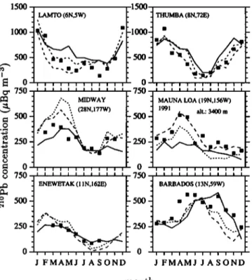
enged and can easily reach high southern latitudes. To compare the scavenging schemes in the tropics where convective precipitation is dominant, we con- sidered six tropical stations in Figure 4c. Not with- standing Midway and Mauna Loa stations, we see lit- tle differences in the concentrations simulated by the three schemes. Springtime concentrations at Midway are overpredicted by schemes RH95 and W88. This is the time of the year when Asian influences are most felt across the North Pacific [Merrill et al., 1989; Harris and Kahl, 1990], coincident with large-scale precipita- tion. The picture is reversed at Mauna Loa where these two schemes reproduce the spring maximum when the
scheme B93-G98 shows no seasonal variation associated
with this time of year. It is noteworthy that concentra-
125 100
75
50 25 0 75 50 25 125PUNTA ARENAS (53S,71W) KERGUELEN (49S,70E)
1991 100 ,' -,
.. .... , '75
' , ,"
'•
'••,
25
i i i i i I i i i i i i i i i i i i i i i i i PALMER (65S,64W) . DUMONT d'Ur. (67S,142E)
1991
,"' ", ,*
1991 ,..
ß
o
. '•',
. o
. . ....
o
.,*' ',* 50
ß ***
'-,,..-' m m m m m
m
i i i i i m i { i i { 0 i { i i i i i i i i I
J FMAMJ J A S OND J FMAMJ J A S OND
month
Figure 4b. Same as Figure 4a but for four stations
28,882 GUELLE ET AL.- INTERCOMPARISON OF AEROSOL WET-SCAVENGING SCHEMES 1500 1000 500 750 500 250 0 750 500 25O
,LAMTO
(6N,SW)
f t THUMBA
(8N'72E)
"
"[-10o0q
ß
[ 0t
'
... 750 ...
:-. MIDWAY I MAUNA
LOA
(19N,
156W)
ß
'",
'• (28N,177W)
.• 1991
/&x•
alt.:
3400
m
-5' ' • 500•
ß '• .•
250
ß.-•.'"•,-'
ß
]
:-....
o ...
i i i i i i i i i i i i ... 750 ...ENEWETAK
(11N,162E)
t BARBADOS
(13N,59W)
500 ß
ß
' - -.,• 250
•o.I I I I I I I I I I I I 0 I ! I I I I ! I I I I I
J FMAMJ JASOND J FMAMJ JASOND
month
Figure 4c. Same as Figure 4a but for six stations located in the tropics.
tions at Mauna Loa (3400 m above sea level (asl)) dur- ing springtime are significantly higher than at Midway, although the distance from the Asian continent (where
most
of the 21øpb
source
is) to Mauna Loa is twice that
of Midway. Clearly, our modeling does not allow to re- solve these discrepancies. An underestimated source of
222Rn,
the precursor
of 21øPb,
over Asia has been sug-
gested to explain the differences at Mauna Loa (P.S. Kasibhatla and N.M. Mahowald, personal communica- tion).
In summary, aside from the local differences depicted in this section and that the tendency scheme W88 has to overpredict high-latitude surface concentrations, the three schemes behave rather similarly at reproducing
the monthly 21øpb concentrations measured near the
surface at most of the sampling stations.
3.3. Vertical Distribution
Figure 5 depicts the respective zonal mean 21øpb con-
centrations as a function of altitude using the three
scavenging schemes. The 21øpb at southern middle and
high latitudes is transported from more northward re- gions where land covers much larger areas and hence
where
21øpb
is much more abundant.
This explains
the
steep north-south gradient encountered in the southern hemisphere. At northern middle and high latitudes, since scheme W88 removes less efficiently the aerosol than the other two schemes, it produces higher surface concentrations. Another significant difference that can be seen is the unrealistically high zonal mean concen- trations produced by scheme RH95 in the middle tropo-
sphere and above. Since scavenging occurs only up to
3.6 km height in that scheme,
the 21øpb
formed
above
contributes
to these high values. In the tropics and
subtropics the main difference is between the B93-G98 scheme Which computes scavenging from the aerosol mass flux entrained in the updrafts, and the other two schemes that depend on the precipitation rates. Un- like the other two schemes the scheme B93-G98, based on mass fluxes, does not show a pronounced minimum concentration around 8 km height. Below, we further compare the model vertical profiles to observations in the tropics.
3.3.1. Comparison between observed and sim-
ulated 2•øpb vertical profiles. To understand the
influence of the different schemes on the vertical dis-
tribution, we have compared the profiles of concentra- tions issued from the three simulations with existing tropospheric measurements. An attempt to compare observed and simulated profiles with four different scav-
enging schemes is described by Lee and Feichter [1995].
•90 -60 -30
...
::,-?:':::•:'""i":
.':.:;:-::21
.'•
..:: :.... • . ::.• .. 0 : '-25 '::::':: :': -•) -(• -30 0 i5 ... . ... ... .. :. .. 0 30 60 .90 ! , , i , . . .[.., .... , .Figure 5. Zonal averages as a function of altitude of
mean annual
21øpb
concentration
(pBq m -3) obtained
with schemes RH95 (top), W88 (middle), and B93-G98 (bottom). Isolines are 25, 50, 100, 150, 200, 300, 400, 500, and 600.
4 -::',• .• •, -- '•:,,. -.::: '--::.-::-::.--..•- ... :. :.---...-• -
4 <' ,:::.-' . .. ... ; :: :: ... •"::-':':. <• ':: ":'"
o 3o • latitude
GUELLE ET AL.' INTERCOMPARISON OF AEROSOL WET-SCAVENGING SCHEMES 28,883 80N 70N 60N 50N 40N ,o 30N o• 20N 10N 10S 20S
120E 140E 160E 180 160W 140W 120W 100W
•
18
•0
2 •
3.•12 14
120E 140E 160E 180
I Moore et al. (Jan. 1968-71, Aug. 1971)
1 to 8 PEM-West A (Sept.-Oct. 1991)
11
to
2•LPi•M-West
B (Feb.-March
1994)
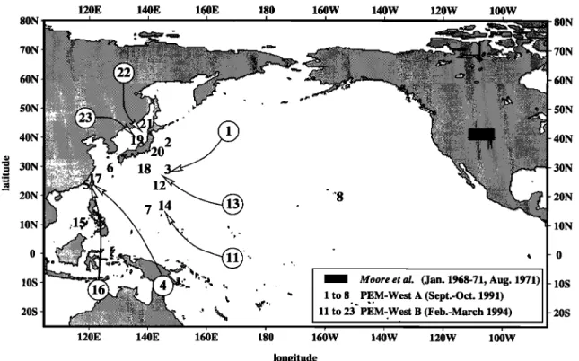
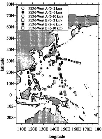
160W 140W 120W 100W 80N 70N 60N 50N 40N 30N 20N I0N 10S 20S longitudeFigure 6. Location of the 2•øPb concentration measurements in altitude used in this study.
The shaded area over North America includes the location of measurements done by Moore et al.
[1973] in January 1968 and 1971 and in August 1971. The numbers correspond to the location of vertical profiles obtained from concentration measurements in altitude during two campaigns over the North Pacific. Each profile is the result of concentrations measured at different heights
during the same flight within approximately 6 hours and which locations are included in the same
model column. Profiles i to 8 are from PEM-West A campaign which took place over the Pacific in September and October 1991 [Dibb et al., 1996]. Profiles 11 to 23 were carried out in February and March 1994 during the campaign PEM-West B [Dibb et al., 1997]. This numbering has been chosen to differentiate in the figure the profiles from the two campaigns, and is increasing with
the sampling
date. To avoid overlapping,
we have displaced
some
of the profile numbers
(inside
circles), where the true location is given by the edge of the associated arrow. Many of the measurements they used were taken in the
stratosphere, and the comparison is complicated by the poor model resolution at these heights and the difficulty to resolve the stratosphere-troposphere exchange.
The shaded area in Figure 6 shows the location of ob-
servations from Moore et al. [1973] over North America.
We have averaged these profiles from two periods: Jan- uary and August. For each month there were only two instantaneous observed profiles, and in the absence of meteorological data for 1971, we used the 1991 simu- lation to compare mean January and August vertical profiles over the model grid box where the measure- ments took place. Vertical profile comparisons are pre- sented in Figure 7. Only scheme B93-G98 reproduces the observed winter profile when synoptic precipitation dominates, although it overestimates the high tropo- spheric concentrations by approximately a factor of 2. No scheme reproduces accurately the slope of the ob- served summer profile. This could be due either to a dif- ferent meteorology in 1971 than during the year 1991 of the simulation or to a poorly resolved convection in the
model. Indeed, Mahowald et al. [1995] have shown, by
comparison of predicted and observed vertical profiles
of 222Rn
concentration,
that the Tiedtke
[1989]
scheme
used in the TM2 causes too high convection during sum-
mer over North America.
To do a more in-depth study of the differences be- tween the scavenging schemes, we compare the model results for the simulations of fall 1991 and spring 1994 to the vertical profiles taken by J. E. Dibb in Sept.-Oct. 1991 during the NASA Pacific Exploratory Mission-
West, Phase A (PEM-West A) expedition [Dibb et al., 1996] and in Feb.-March 1994 during the PEM-West B expedition [Dibb et al., 1997], both taking place mostly
over western North Pacific. In all cases we are able to
compare these profiles to the model results for the ana- lyzed meteorological conditions of the same days. The comparison to the observed vertical profiles of concen- trations consists in selecting the locations included in the same model grid column where the plane flew at
different heights during the same flight, i.e., approxi-
mately within 6 hours. The output concentrations in the model are set every 6 hours in order to compare as accurately as possible observed and simulated instanta- neous concentrations. We show in Figure 6 the location
28,884 GUELLE ET AL.. INTERCOMPARISON OF AEROSOL WET-SCAVENGING SCHEMES 16 14 12 scheme
R•95
t t Central USA (42N,104W) January 1968, 1971 .: \ : \/•".,...
',
/
scheme :•1 W88 :' ... i i scheme [fi B93-G98 .:" observ ., .]...[...[., , [, , . 100 200 300 400 500 2]øpb conc. (gBq m -3 ) 0 0 Central USA (40.5N-42N, 103.5W-111W) August 1971 300 600 900 1200 2]øpb conc. (gBq m '3 )Figure 7. Comparison between observed and predicted
vertical
profiles
of 21øPb
concentrations
(ttBq
m -a) with
the three schemes over North America for January and
August. The observed profiles (thick solid line) are
both the combination of two instantaneous profiles ob-
tained in 1968 and/or 1971. The simulated profiles are
monthly averages for January and August 1991. The dashed line with circles corresponds to scheme RH95, dotted line with open squares to scheme W88, and thin solid line with solid squares to scheme B93-G98.
and descents do not allow to have profiles aJong all the
tracks that were flown). We could assemble eight pro-
files for PEM-West A, and thirteen for PEM-West B. Figures 8a-8c show the comparison of the vertical pro- files obtained by the three schemes with those observed; Figure 8a is for PEM-West A and Figures 8b and 8c for
PEM-West B.
The PEM-West A campaign took place in late sum- mer to early fall, when convective activity dominates over the Pacific. As already discussed, we can no- tice in Figure 8a that predicted concentrations with scheme B93-G98 are often higher than with the other two schemes, indicating a less efficient scavenging by convective precipitation. Leaving profile 2 for which the discrepancy between observed and predicted concentra- tion seems not to depend on the scavenging scheme, we see in Figure 8a that the scheme B93-G98 is in better agreement with observations than the other two schemes for all flights except for flight 7.
The comparison between two profiles (1 and 3) taken
over the same location shows a threefold increase of
the 2•øPb concentrations at 8.5 km altitude. This is the result of a stratospheric air intrusion which pen-
etrates deeply in the troposphere [see Browell et al., 1996, Plate 2]. The model does not account for this
kind of problem because of its very poor vertical res- olution in the stratosphere, preventing from simulat-
ing accurately the troposphere-stratosphere exchanges. This explains why this tropopause fold is not simulated by the model, yielding an underestimate of the high-
altitude 2•øPb concentration of profile 3.
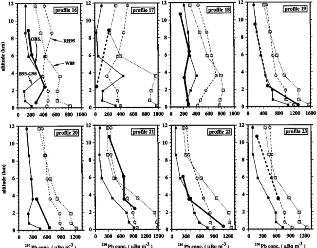
The PEM-West B campaign gives an additional in- formation since it took place at a time of the year
(late winter to early spring) when synoptic precipita-
tion is important at midlatitudes. Moreover, circula- tion patterns were also different than for the PEM-West A period, with the Japan jet responsible for most of the Asian continental outflow extending farther south and being stronger in intensity in Feb.-Mar. than in
Sep.- Oct. [Gregory et al., 1997; Merrill et al., 1997].
Considering the convective and synoptic precipitation amounts for that period according to the analyzed pre- cipitations from NCEP, we can distinguish profiles ob- tained in regions where convective precipitation domi-
nates (profiles 11 to 15, Figure 8b) versus regions where synoptic precipitation is more important (profiles 16 to 23, Figure 8c). Aside from profile 15 for which no
scheme succeeds in reproducing the observed concen- trations, schemes RH95 and W88 overpredict the pro- files by roughly a factor of 2, whereas scheme B93-G98 comes in closer agreement with the observations. In
contrast to the results obtained with PEM-West A mea-
surements, concentrations predicted with scheme B93-
G98 over convective areas are less than those with the
other two schemes. This is attributable to the synoptic precipitation band that spreads from Japan to south-
eastern China and removes efficiently •øPb en route
from the Asian continental source to more tropical re- gions where convective precipitation dominates.
This efficiency at scavenging is clearly observed in
regions where synoptic precipitation dominates (Fig- ure 8c). Schemes RH95 and W88 overestimate the ob- served concentrations, whereas scheme B93-G98 shows a much better agreement, except for profile 17. Again, the disagreement shown by scheme B93-G98 for pro- file 21 is attributable to a strong tropopause fold the
model does not simulate. This conclusion was reached
by Dibb el al. [1997] looking at O3 and aerosol-scattering
vertical profiles from a UV-DIAL instrument. These vertical distributions clearly show a deep intrusion of stratospheric air which can explain the twofold increase of observed 2•øPb concentration at 10.7 km altitude between profiles 21 and 23 which were taken within 6
hours.
It is evident from these different profile comparisons that schemes RH95 and W88 are not efficient enough in
removing
2•øPb from the atmosphere
via synoptic
pre-
cipitation. However, we can notice in Figures 7 and 8c
the reverse trend between middle/high and low tropo-
sphere for the profiles simulated by these two schemes.
In fact, whereas
scheme
RH95 exhibits
greater 2•øPb
concentrations in the high troposphere due to the lack of scavenging above 3.6 km altitude, it shows smaller
2XøPb concentrations in the low troposphere, because
GUELLE ET AL- INTERCOMPARISON OF AEROSOL WET-SCAVENGING SCHEMES 28,885
0 100 200 300 400 500 0 300 600 900 1200 0 100 200 300 400 500 0 50 100 150 200 250 300
',1
profile
$1
e
61
/.? profile
7
, I profile
81
10 10 10 10 8 8 8 8 ,,
• 4
!
4
4
4
•-•..
2 • 2
.,I 2
2
0 . , . 0 .,,, 0 . ,. 0 0 200 400 600 800 1000 0 300 600 900 1200 0 100 200 300 400 0 100 200 30021o
Pb
conc.
( gBq
m
'3 )
21o
Pb
conc.
( gBq
m
'3 )
2•o
Pb
conc.
( gBq
m
'3 )
2•o
Pb
conc.
( gBq
m
'3 )
Figure 8a. Comparison
of instantaneous
vertical
profiles
of 2•øPb
concentrations
(ttBqm
-a)
predicted
by the three schemes
with vertical
profiles
observed
over
the western
North Pacific,
in
September-October
1991 during
the PEM-West
A campaign.
The different
lines correspond
to
the cases
in Figure
7. The observed
profiles
are plotted as solid
circles
for the measurements,
as
well as linear interpolation lines between two consecutive samples in altitude. This line is dotted when two consecutive samples are distant by more than 5 km in altitude.
guish in-cloud scavenging from interception below the
cloud base.
3.3.2. Quantitative comparison. In order to quantify the ability of each of the three schemes to simu- late the vertical distribution of 2•øPb we have first com-
12 12
t iprofile
11]
• ../.rn,,,•
f l•'"',
]Prøfile
12]
I
i ', [protile 13 I10
]B93-G98
•/
::..:'
/ l•
10
• 4
• •95
0
...
}
200 400 600 0 200 400 600 800 0 300 600 900 1200
Pb
conc.
( laBq
m
'3 )
2•o
Pb
conc.
( gBq
m
'3 )
21o
Pb
conc.
( laBq
m
'3 )
pared the vertical gradients of concentrations measured and simulated. For this purpose we have calculated 47 gradients of observed 2•øPb concentrations as a function of height for each couple of two consecutive altitudes
of samplings deduced from all the profiles presented
', I profile 14 I 8 2 .... 1•:o