HAL Id: insu-01355054
https://hal-insu.archives-ouvertes.fr/insu-01355054
Submitted on 22 Aug 2016
HAL is a multi-disciplinary open access
archive for the deposit and dissemination of
sci-entific research documents, whether they are
pub-lished or not. The documents may come from
teaching and research institutions in France or
abroad, or from public or private research centers.
L’archive ouverte pluridisciplinaire HAL, est
destinée au dépôt et à la diffusion de documents
scientifiques de niveau recherche, publiés ou non,
émanant des établissements d’enseignement et de
recherche français ou étrangers, des laboratoires
publics ou privés.
Tensor deconvolution: A method to locate equivalent
sources from full tensor gravity data
Valentin Mikhailov, Gwendoline Pajot, Michel Diament, Antony Price
To cite this version:
Valentin Mikhailov, Gwendoline Pajot, Michel Diament, Antony Price. Tensor deconvolution: A
method to locate equivalent sources from full tensor gravity data. Geophysics, Society of Exploration
Geophysicists, 2007, 72 (5), pp.I61-I69. �10.1190/1.2749317�. �insu-01355054�
Tensor deconvolution: A method to locate
equivalent sources from full tensor gravity data
Valentin Mikhailov
1, Gwendoline Pajot
2, Michel Diament
2, and Antony Price
3ABSTRACT
We present a method dedicated to the interpretation of full tensor共gravity兲 gradiometry 共FTG兲 data called tensor decon-volution. It is especially designed to benefit from the simulta-neous use of all the FTG components and of the gravity field. In particular, it uses tensor scalar invariants as a basis for source location. The invariant expressions involve all of the independent components of the tensor. This method is a ten-sor analog of Euler deconvolution, but has the following ad-vantages compared to the conventional Euler deconvolution method:共1兲 It provides a solution at every observation point, without the use of a sliding window.共2兲 It determines the structural index automatically; as a consequence, the struc-tural index follows the variations of the field morphology.共3兲 It uses all components of the measured full gradient tensor and gravity field, thus reducing errors caused by random noise. It is based on scalar invariants that are by nature insen-sitive to the orientation of the measuring device. We tested our method on both noise-free and noise-contaminated data. These tests show that tensor solutions cluster in the vicinity of the center of causative bodies, whereas Euler solutions bet-ter outline their edges. Hence, these methods should be com-bined for improved contouring and depth estimation. In addi-tion, we use a clustering method to improve the selection of solutions, which proves advantageous when data are noisy or when signals from close causative bodies interfere.
INTRODUCTION
The history of gravity gradiometry dates back to 1886 when Loránd Eötvös constructed his first torsion balance gradiometer. It was the first potential field measurement device widely used in oil exploration共e.g. Bell and Hansen, 1998; Pawlowski, 1998兲. The first
mapping of oil-bearing anticline structure was performed in Gbely, Slovakia, in 1916共Szabó, 1998兲. In the 1930s, gradiometers were re-placed by gravimeters and gravity measurements became easier, faster, and cheaper. Because gravity data were more easily interpret-able in the precomputer era, this method was widely used.
The development of high-performance moving-platform full ten-sor gradiometry共FTG兲 systems has led to the rebirth of gravity gra-diometry. The first systems measuring all components of the gravity gradient tensor共FTG兲 were developed in 1970s 共Jekeli, 1993; Bell et al., 1997兲. In the late 1980s, these instruments were, for the first time, implemented in exploration geophysics 共e.g. Bell and Hansen, 1998兲. Recently, many examples of successful applications of FTG data in mineral exploration and oil prospecting have been reported 共e.g. Pawlowski, 1998; Zhdanov et al., 2004兲. Gravity gradiometry applications, however, are not restricted to prospecting purposes. In-deed, the European Space Agency is planning to launch the GOCE 共Gravity Field and Steady-State Ocean Circulation Explorer兲 satel-lite in late 2007 with a gradiometer onboard共ESA, 1999兲. Tensor data will then be used in combination with GPS tracking to improve models of the global gravity field and geoid. This shall lead to un-precedented accuracy and spatial resolution, thus allowing new re-gional and local geodynamical studies.
In many studies, FTG data are used to calculate the enhanced gravity field gz, which contains shorter wavelength components in comparison to gravimetry data. This allows a more detailed mapping of subsurface structures, such as the lower boundary of salt domes 共Jorgensen and Kisabeth, 2000; Routh et al., 2001兲. Using the en-hanced second vertical derivative of the potential Uzzcalculated from FTG data, joint inversion of seismic and FTG data is also per-formed共e.g. O’Brien et al., 2005兲. Several new techniques for FTG data processing and interpretation have been recently suggested 共e.g. Condi and Talwani, 1999; Jorgensen and Kisabeth, 2000; Zhang et al., 2000; Li, 2001a, b; Routh et al., 2001; Lyrio et al., 2004; Zhdanov et al., 2004; and While et al., 2006兲. However, theory and methods for FTG data processing and interpretation that combine all FTG components and the gravity field are still challenging. We
be-Manuscript received by the Editor July 7, 2006; revised manuscript received April 6, 2007; published online July 18, 2007.
1Institut de Physique du Globe de Paris, Paris, France and Institute of Physics of the Earth RAS, Moscow, Russia. E-mail: [email protected]. 2Institut de Physique du Globe de Paris, Paris, France. E-mail: [email protected]; [email protected].
3Total E&P, Non-seismic Geophysics, Paris, France. E-mail: [email protected].
© 2007 Society of Exploration Geophysicists. All rights reserved.
lieve that new marine, airborne, and space FTG measurement tech-niques call for the development of new methods of data processing and interpretation. Indeed, even the transformation of FTG data into enhanced gravity leads to the loss of useful information.
In this paper, we present a method to locate equivalent sources us-ing FTG data. It is based on the same principles as Euler deconvolu-tion, thus we call this method tensor deconvolution. It uses tensor scalar invariants and, thus, should be robust to errors caused by im-perfect orientation of the measuring device. Moreover, because it uses the complete set of components of the FTG tensor, it is resistant to random noise in the different measurement channels. Contrary to the traditional Euler deconvolution method, it allows an automated estimate of the structural index and does not require a sliding win-dow. Moreover, although this is not the first attempt to enhance Euler deconvolution by the use of gravity gradient data, this method differs from the previously published work dedicated to this effort because it uses all the measured values simultaneously, and only these val-ues.共For example, Zhang et al., 2000, applied Euler deconvolution to FTG data considering different lines of the FTG tensor compo-nents separately. Their approach requires the calculation of the hori-zontal derivatives gxand gyof the gravity potential U.兲
After recalling the fundamentals of Euler deconvolution and de-veloping the mathematical relationships on which the algorithm is based, we present this algorithm and apply it to synthetic examples. It appears that our method may be particularly efficient at resolving the depths of multiple sources in the presence of noise.
TENSOR DECONVOLUTION Mathematical background
Let us first briefly recall the principle of Euler deconvolution. By definition, a real function f is a homogeneous function of degree n when, for any t, it obeys the equation,
f共tx,ty,tz兲 = tnf共x,y,z兲. 共1兲
According to this definition, the gravity and magnetic fields caused by some simple sources are homogeneous functions of the spatial coordinates. In particular, this equation is valid共see, for example, Blakely, 1995兲 for gravity 共and magnetic兲 anomalies associated with point sources and lines of sources共or, in the magnetic case, point poles and point dipoles and lines of poles and dipoles兲. The location of a point source共,,兲 in 3D, or the location of a line source 共,兲 in 2D, can be found from the following equation共Euler equation兲:
共x −
兲
f
x +共y −
兲
f
y + 共z − 兲
f
z = − N共f共x,y,z兲 − A兲, 共2兲where N = −n is the structural index, which depends on the type of the body, and A is an unknown constant level in a measured field 共Th-ompson, 1982; Reid et al., 1990兲. To solve equation 2, the Euler de-convolution method uses a sliding window of data points. At least four data points are required in this window, because we are solving for four unknown parameters:,,, and A 共e.g., Reid et al., 1990兲.
Strictly speaking, line and point sources are the only causative bodies that obey the Euler equation of homogeneity. Nevertheless, Euler deconvolution can also be applied to a deep body of arbitrary shape, where the anomaly is close to that of a point source or a line of sources, with corresponding structural indices N = 2 or N = 1 共ex-amples of the structural indices corresponding to different causative
sources are given by Stavrev, 1997兲. Moreover, Euler deconvolution has proven successful for edge detection of real bodies, especially simple ones having close to vertical sides. Furthermore, several bod-ies may obey the Euler equation under specific conditions. For ex-ample, equation 2 is valid for a dike共vertical or inclined兲 or a finite step when its offset is considerably smaller than its depth共Li, 2003兲. When the Euler method is applied to real 3D bodies, the obtained so-lutions very often either trace near vertical edges of causative bod-ies, or point to their center of mass.
Results of Euler deconvolution are sensitive to the choice of the structural index, as well as of the size and location of the sliding win-dows共Fairhead et al., 1994兲. In practice, several structural indices are tried, and the one providing results fitting to known geological and seismic data, or having good clustering properties, is kept共for an exhaustive study of the discrimination techniques to use in Euler de-convolution methods, see Fitzgerald et al., 2004兲. However, errors in the estimated depth of the sources occur when the index is inappro-priate, and the a priori choice of a single constant index is obviously inappropriate when multiple sources with different geometries inter-fere. The depth estimation can be improved using additional analyti-cal constraints, namely the property of invariance under rotation of homogeneous functions共Mushayandebvu et al., 1999兲. This pro-vides additional equations and the so-called “extended Euler decon-volution method” provides better depth estimation than traditional Euler. Nabighian and Hansen共2001兲 mention that additional equa-tions permit the elimination of the structural index N between pairs of equations, yielding a system of two equations at each point, which are still linear in,, and, do not contain N explicitly, but are bilin-ear in the field variables. Discussions on methods to estimate the structural index can be found, for example, in Slack et al.共1967兲, Steenland共1968兲, Barbosa et al. 共1999兲, and Martelet et al. 共2001兲. As recalled by Li共2003兲, most methods to determine the geometry of the source共without deducing it from geology兲 and, thus, to guide the choice of an adequate structural index, are based on computing de-rivatives, and this calculation is well known to be numerically unsta-ble, especially in the presence of noise. On the synthetic examples below, we compare our suggested tensor deconvolution method with different versions of the Euler technique, even though the compari-son of extended and conventional Euler deconvolution is beyond the scope of this paper. When applying the conventional and extended Euler method we assigned the correct structural index correspond-ing to synthetic sources used. We believe that in this case共contrary to realistic exploration situations where the structural index is un-known兲 extended Euler methods provide results close to the ones ob-tained by conventional Euler.
Zhang et al.共2000兲 adapted the extended Euler deconvolution method to gravity gradient data. This allows the use of measured rather than computed derivatives, but their method requires the cal-culation from gzof derivatives gxand gyof the gravity potential along two horizontal coordinate lines, which is also known to be numeri-cally unstable, especially in the presence of regional long-wave-length components. We hereafter describe a method to use the gravi-ty tensor invariants computed from measured gravigravi-ty gradients. Un-like previous methods, it combines the following advantages: • Instead of a priori choosing a constant structural index, the index,
which is related to the geometry of the source, is computed at ev-ery point directly from the data. The constraint brought by the knowledge of the geometry of the source to aid its localization is
therefore deduced from the data and suitable for large data sets where the structural index is likely to vary.
• It does not require the use of a sliding window or the computation of derivatives, and, thus may be less sensitive to numerical insta-bilities caused by noise.
Let us now recall some fundamentals about the gravity gradient tensor. We use a Cartesian system of coordinates共x,y,z兲 with the
z-axis directed downwards and the x-axis directed northwards. The
gravity gradient tensor in the共x,y,z兲 frame can then be written in the form, T =
冨
Uxx Uxy Uxz Uyx Uyy Uyz Uzx Uzy Uzz冨
, 共3兲where U is the gravity potential, and for all pair共␣,兲 in 兵x,y,z其 U␣
=2U/␣. In the following text, we denote by g
␣the first
deriva-tive of the gravity potential U along direction␣. Traditionally, gradi-ents U␣are expressed in Eötvös unit E, with 1E = 10−9s−2, and g
␣in
mGal, with 1 mGal = 10−5ms−2. Because gravity is a conservative
field and because of the commutability of the differential operators, the tensor is symmetric共U␣= U␣兲 and its trace is equal to zero
out-side of the causative sources. Thus, in free space, the tensor has only five independent components. Current commercial gradiometers, such as the Bell Geospace FTG, provide all off-diagonal and two di-agonal components of the upper triangle of the gradient tensor, the third diagonal component being calculated from the two others 共While et al., 2006兲. The tensor is fully defined from these five mea-surements.
Following Pedersen and Rasmussen共1990兲, we now investigate the scalar invariants of the tensor. Let us consider the eigenvectors vi
and the eigenvaluesiof the tensor T. Being real and symmetric,
tensor T can be written in the form共Pedersen and Rasmussen, 1990, equation 9兲:
VtTV =⌳, 共4兲
where V =关v1,v2,v3兴 is a matrix, the columns of which are
eigen-vectors of T, and⌳ is a diagonal matrix containing the three eigen-values of the tensor. The superscript t denotes the transposition of tensor T. Physically, with the origin of the coordinate system at the observation point, equation 4 means that one can find three princi-pally different possible orthogonal rotations of the initial system of Cartesian coordinates共x,y,z兲, such that in the new coordinate sys-tem all off-diagonal elements vanish. The eigenvectors videtermine the axes共known as the principal axes兲 of the new coordinate system. By definition, the tensor eigenvalues are the roots of the characteris-tic equation:
3− I0
2+ I1
− I2= 0, 共5兲where the Iicoefficients are the scalar invariants of the tensor T, the expressions of which involve only the tensor eigenvalues.
Pedersen and Rasmussen共1990兲 introduced the dimensionless variant ratio I associated with tensor T that we call hereafter the
in-variant ratio:
I = −共I2/2兲2/共I1/3兲3,0 ⱕ I ⱕ 1. 共6兲
The invariant ratio I is equal to zero when the field is invariant along some direction共2D causative source兲 and equal to 1 for radially sym-metric fields共e.g., a point source, see below兲.
We now develop the main relationships that allow us to compute the coordinates of a point source and a line source using the invariant ratio and eigenvalues.
Point source
The gravity potential that is associated with a point source is U = GM /R, where G is the gravitational constant, M is the mass of the point source, R =
冑
共 − x兲2+共− y兲2+共 − z兲2,共x,y,z兲 are thecoordinates of the observation point, and共,,兲 those of the point source. We denote by1the maximal by absolute value eigenvalue
of the tensor, and v1the corresponding eigenvector. Following
Ped-ersen and Rasmussen共1990兲 we get, with our sign convention,
1= 2GM /R3 and v1=共
− x,
− y, − z兲/R, 共7兲where v1is directed from the observation point towards the source.
Thus, the eigenvector components assign the three directional an-gles to the source, but because v1is a unit vector, they do not assign
the distance to it. To find the three coordinates of the source, we can use the formula for the gravity anomaly gz共measured or enhanced/ calculated, see the introduction兲, which is equal to
gz= GM共 − z兲/R3. 共8兲
Thus, using equations 7 and 8, we compute the depth to the point source:
− z = 2gz/
1, 共9兲and the remaining共 − x,− y兲 coordinates can now be found from the components of vector v1. As a result, using all values of the full
gradient tensor to compute1and knowing the value of the gravity
anomaly in one point, it is possible to find the position of an equiva-lent point source.
Moreover, the eigenvector v1determines a new Cartesian frame
共O1,x1,y1,z1兲, whose origin O1is at an observation point and where
the z1-direction coincides with v1. Thus at the origin O1共former
共x,y,z兲 point兲 we have:
1= Uz1z1, gz1= GM /R2, 共10兲and equation 9 transforms to:
共z1−兲Uz1z1= − 2gz1. 共11兲
In the new coordinate system, derivatives Ux1z1and Uy1z1are equal to zero. Therefore, equation 11 is equivalent to the Euler equation for a point source with structural index 2.
For a line source directed along the x-axis
We denote by M the mass of the line source per unit length. Then, the gravity potential is U = − 2GM ln共R兲 共Telford et al., 1990兲 and using the same notations as for the point source, and still following Pedersen and Rasmussen共1990兲, we have
1= 2GM /R2 and v1=共0,
− y, − z兲/R. 共12兲Unit vector v1is directed from the observation point to the nearest
point of the line source共it is obvious that all these relationships are valid for an arbitrary orientation of the line source兲.As before, to find
the coordinates of the source we use the gravity anomaly gzwhich is, for a line source, gz= 2GM共 − z兲/R2, and thus we find the depth of the line source:
− z = gz/
1. 共13兲Again, equation 13 is analogous to the Euler equation with the struc-tural index equal to 1.
Extending formulas to real 3D bodies
Considering equations 11 and 13, we now suggest a general for-mula valid for elongated and isometric bodies, as follows:
= z + 共1 + I兲gz/
1, 共14兲or, equivalently,
= z + Ngz/
1. 共15兲Indeed, according to Pedersen and Rasmussen共1990兲 a point source has an invariant ratio I = 1, which provides the structural index N = 2. For a line source, the invariant ratio I is zero, thus N = 1. Equa-tion 14 thus links equaEqua-tions 11 and 13. For other sources, there is no strict analog of the Euler formula, instead we check our equation 14 numerically using fields generated by different causative sources. Because equation 14 is not the only way to relate the structural index to the invariant ratio I, further numerical studies are, of course, nec-essary. Using synthetic examples we investigated different power functions N = 1 + Ik, but for k ranging from 1 to 10, results appeared to be very close. Invariants of a tensor are, by definition, independent of the vector basis where the components of the tensor are expressed. Thus, we expect our method to be less sensitive than others to the
problems of misorientation of the measuring device. However, we do not investigate this question further in the present paper. We also do not address here the problem that some measured FTG tensor components are probably more noisy than others, as described by While et al.共2006兲.This would be a subject for a separate detailed in-vestigation. We can now present the procedure for contouring caus-ative sources and estimating their depths from FTG data.
Algorithm for the tensor deconvolution
The algorithm for the tensor deconvolution includes the following steps:
1兲 Calculation of eigenvalues, eigenvectors, tensor invariants, and the invariant ratio I at every observation point and estima-tion of the structural index according to equaestima-tion 14
2兲 Calculation of the coordinates of an equivalent source using the maximal by absolute value eigenvalue and corresponding ei-genvector
3兲 Filtering the solutions using approaches developed for Euler deconvolution共limits along coordinates, distance from obser-vation point to the equivalent source etc兲
At step 1 we used the standard procedure suggested in Press et al. 共1992兲. In our practical calculations, we also applied two additional approaches for the step 3 of the algorithm: solutions are rejected when their horizontal distance L from the observation point is K times larger than their depth z共K is a user-determined parameter兲, and we apply clustering of the solutions as suggested by Mikhailov et al.共2003兲. The first criterion means that we are looking for solu-tions situated below the observation point within the cone whose top angle␣ is ␣ = 2 tan−1共K兲. This criterion appeared to be very
effi-cient. Different possible criteria to discriminate between the solu-tions are widely discussed by Fitzgerald et al.共2004兲.
DISCUSSION
In this section, we discuss the efficiency of Euler and tensor de-convolution in locating causative sources on synthetic examples. Because for isolated bodies both Euler and tensor deconvolution work well, we focus on examples of complex fields共extensive inter-ference of signals, high noise level兲. For the first two examples, we show the invariants of the tensor corresponding to the investigated structures, as well as the three amplitudes of the analytic signal de-rivatives共seeAppendix兲 and discuss their contouring properties. We then compare the efficiency of different versions of the Euler decon-volution method and of our method to locate the causative sources. The last example shows the ability of the algorithm to distinguish in-terfering 3D sources which do not obey the Euler equation.
Example 1: Line of point sources
We consider the gravity anomaly caused by 21 point sources situ-ated, one per kilometer, below the x-axis, between x = −10 km and
x = 10 km, and all at a depth of 2 km. On the figures illustrating this
example, only the x⬎0 part of the plane is shown, because the gravi-ty field is symmetrical with respect to the y-axis.
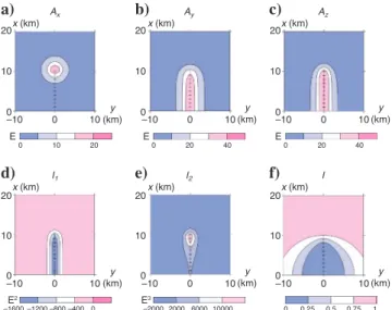
Figure 1 shows the components of the gradient tensor and the gravity anomaly gzcaused by these point sources. Figure 2 shows the amplitudes of the analytic signal derivatives Ax共Figure 2a兲, Ay 共Fig-ure 2b兲 and Az共Figure 2c兲, the first 共Figure 2d兲 and second 共Figure
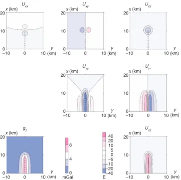
x (km) –10 0 10 20 10 0 x (km) –10 0 10 –10 0 Uxx Uxy Uxz 10 20 10 0 x (km) y (km) 20 10 0 x (km) mGal E –10 0 10 20 10 0 8 4 0 –10 0 gz Uzz 10 x (km) 20 10 0 40 20 10 5 0 –5 –10 –20 –40 x (km) –10 0 10 –10 0 Uyy Uyz 10 20 10 0 x (km) 20 10 0 y (km) y (km) y (km) y (km) y (km) y (km)
Figure 1. FTG components U␣共in E兲 and the gravity field gz共in mGal兲 caused by 21 point sources situated, one per kilometer, below the x-axis, between x = −10 km and x = 10 km, and all at a depth of 2 km. Because of symmetry, only the northern part共xⱖ0兲 of the resulting fields are shown. All distances are in kilometers. The indi-vidual effects of the point sources cannot be seen in either the gravity field or its derivatives.
2e兲 invariants of the tensor, and the invariant ratio 共Figure 2f兲. Figure 3 shows the results of our method without共Figure 3a兲 and with 共Fig-ure 3c兲 clustering, those of traditional Euler deconvolution with the clustering selection criterion共Figure 3b兲, window size 3⫻3 km, and a constant structural index N = 1 corresponding to a linear source. Isolines of gzare plotted in the backgrounds of Figure 3a–c.
The isolines of Ay共Figure 2b兲 and Az共Figure 2c兲, as well as the first invariant共Figure 2d兲 contour the set of the causative sources 共these functions are similar because the line of monopoles stretches along the x-axis兲. Analytic signal Ax共Figure 2a兲 and the second in-variant共Figure 2e兲 are maximal over the edge of the line of sources. The invariant ratio I共Figure 2f兲 is close to 0 above the line of sourc-es, and close to 1 far from it. Thus the structural index N = I + 1 var-ies over the area. Being calculated with this varying structural index, the tensor solutions from equation 14共Figure 3a兲 cluster more densely than the conventional Euler solutions computed with the constant a priori structural index N = 1共Figure 3b兲. Moreover, the tensor solutions are located in a narrower depth range than the con-ventional Euler ones. Thus, we conclude that in this example, our method better localizes the sources than the conventional Euler de-convolution method.
If, in addition, we use a clustering selection criterion of the tensor solutions共Figure 3c兲, we can even isolate all point sources, but the outermost solutions are slightly shifted toward smaller x共northing兲 values, in comparison to the corresponding point sources. This is a surprising result considering that the depth of the sources is twice the distance between them. However, this result is achieved in absence of any kind of noise.
Example 2: Noise sensitivity
In this example, we investigate a field corresponding to a rectan-gular prism. This structure is far from geologically realistic, but has the advantage of being a 3D isometric body that does not obey the Euler equation. This example allows testing of equation 14. To apply
the conventional Euler deconvolution method, we need to assess the structural index corresponding to a prism. Zhang et al.共2000兲 men-tions that before substitution of integral limits, the gravity field of a rectangular block resembles a homogeneous function with the struc-tural index N = −1. However, the full formula with integer limits does not obey the Euler equation. Moreover, a negative structural in-dex does not fit any potential function. Indeed, an inin-dex N = −1 cor-responds to a function growing toward infinity.
Because at large distances the gravity effect of a rectangular prism is close to that of a point mass, its structural index approaches N = 2 as the distance tends to infinity. At shorter distances the structural in-dex N = 1 corresponding to a small-amplitude step can be used. 共Note that this supports the idea of an effective structural index changing with the distance from a source兲. For this example, we choose to apply the conventional and extended Euler deconvolution method with a constant a priori structural index N = 2.
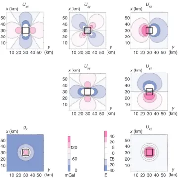
The gravity field and its derivatives are calculated for a rectangu-lar body of 10⫻10 km horizontal dimensions, stretching down from 2 to 30 km and having a density contrast equal to 1 g/cm3.
Figure 4 shows the tensor components and gzassociated with this structure. Figure 5 shows the amplitudes of the analytic signal deriv-atives Ax共Figure 5a兲, Ay共Figure 5b兲, and Az共Figure 5c兲, the first 共Figure 5d兲 and second 共Figure 5e兲 invariants of the tensor, and the invariant ratio共Figure 5f兲. Figure 5a and b demonstrate the selective directional sensitivity of the Axand Aycomponents, which allows
x (km) y (km) –10 0 10 20 –1600 –1200–800 –400 0 –2000 2000 6000 10000 0 10 –10 0 20 40 0 10 –10 0 20 40 0 10 –10 0 10 –10 0 10 –10 0 10 20 10 0 20 10 0 20 10 0 20 10 0 20 10 0 20 10 0 x (km) y (km) Ax x (km) y (km) E
a)
b)
Ayc)
Az E E x (km) y (km) x (km) y (km) I1 x (km) y (km) E2 E3d)
e)
I2f)
I 0 0.25 0.5 0.75 1Figure 2. Amplitude of the analytic signal derivatives, invariants of the gravity gradient tensor, and invariant ratio I for the example shown on Figure 1.共a兲, 共b兲, and 共c兲 The amplitude of the analytic sig-nals derivative Ax, Ay, Azin Eötvös units;共d兲 and 共e兲 show the first and second nonzero invariants共in E2for I
1and E3for I2兲; and 共f兲
shows the dimensionless invariant ratio I. Notice the selective sensi-tivity of these various transforms.
x (km) y (km) 10 0 1 2 1 2 4 10 20 10 0 Tensor solutions Depth in km 1.9 to 2 2 to 2.3
a)
x (km) y (km) –10 0 1 2 1 2 4 10 20 10 0 Tensor + clustering Depth in km 1.9 to 2 2 to 2.3c)
x (km) y (km) –10 0 1 2 1 2 6 10 20 10 0 Euler + clustering Depth in km 1.9 to 2 2 to 2.3 2.3 to 4.3b)
–Figure 3. Comparison of tensor and Euler deconvolution for the ex-ample illustrated by Figures 1 and 2.共a兲 The results of tensor decon-volution,共b兲 the Euler solutions after selection and clustering, and 共c兲 the tensor solutions selected by clustering.All figures are with the gravity field gzin the background. Blue squares, red crosses, and black triangles indicate different depth intervals in kilometers. No-tice that Euler solutions共b兲 form a wider cloud than the tensor solu-tions共a兲. Tensor solutions 共a兲 are located close to the sources. After the clustering of the tensor solutions共c兲 all point sources are recog-nized, though the outermost solutions are shifted to smaller x values with respect to the corresponding point sources. The depths of the solutions are then very close to the real depth of 2 km.
improved outlines of the different edges of the causative bodies. We can also notice the variation of the invariant ratio I above the vertical sides of the prism共Figure 5f兲.
First we add Gaussian random noise with zero average and stan-dard deviations of 1 mGal and 1 E to the gravity field and to all FTG
components, respectively共Figure 6兲. Then we investigate the effect of noise with larger standard deviations, 3 mGal and 7 E, respec-tively共Figure 7兲.
Figure 6 shows the results of our method 共Figure 6a兲 and of conventional Euler deconvolution共Figure 6b兲 with window size 3⫻3 km. For the tensor deconvolution, solutions were selected us-ing two criteria:
1兲 Solutions are required to have positive depth
2兲 Solutions whose horizontal distance from the observation point is K-times larger than their depth are rejected共we used K = 1, thus looking for solutions situated below the observation point, within the cone with top angle 90°兲
For the low-noise example, we restricted the conventional Euler de-convolution method, used as a comparison, by applying both routine selection and clustering. This was necessary because Euler solutions were more widely dispersed.
Figure 6a and b demonstrate that our method better locates the center of the anomalous body, whereas conventional Euler solutions better identify its edges. This suggests that these methods are com-plementary and can be applied simultaneously to better locate caus-ative bodies. The tensor solutions are, however, better at determin-ing a more accurate depth for the causative body modeled here.
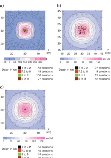
When the level of noise increases共Figure 7a-c兲 the depth accuracy of the conventional Euler solutions increases drastically, and the edges of the body are not well outlined共Figure 7b兲. Though almost the same selection criterion are applied in the cases shown on Fig-ures 6a and 7a, the tensor solutions remain very densely clustered in the center of the body, being distributed in a narrow depth range. To better outline the causative source by conventional Euler and clus-tering, we applied stronger selection criteria, thus considerably re-ducing the number of solutions共Figure 7b兲. Very strong selection criteria applied to extended Euler deconvolution 共LCT software, structural index 2, and window size 36⫻36 points兲 result in a very dense deep cluster situated within a narrow depth interval共Figure
x (km) y (km) 10 20 30 40 50 50 40 30 20 10 10 20 30 40 50 50 40 30 20 10 10 20 30 40 50 50 40 30 20 10 10 20 30 40 50 50 40 30 20 10 10 20 30 40 50 50 40 30 20 10 10 20 30 40 50 50 40 30 20 10 10 20 30 40 50 50 40 30 20 10 x (km) y (km) Uxx Uxy Uxz x (km) y (km) x (km) mGal E y (km) 120 60 0 gz Uzz x (km) y (km) 40 20 5 0 ñ 5 –20 –40 x (km) y (km) Uyy Uyz x (km) y (km)
Figure 4. FTG components U␣共in E兲 and gravity field gz共in mGal兲 caused by a rectangular body of horizontal dimensions 10⫻10 km. The top is at 2 km and the bottom at 30 km, excess density is 1 g/cm3. The solid square on the plots shows the contour of the
caus-ative body. x (km) y (km) 10 0 40 80 120 160
–6E+004 –4E+004 –2E+004
20 30 40 50 50 40 30 20 10 10 20 30 40 50 50 40 30 20 10 10 20 30 40 50 50 40 30 20 10 x (km) y (km) Ax x (km) y (km) E E
a)
b)
Ayc)
Az 0 80 160 240 E 0 80 160 240 E x (km) y (km) 10 20 30 40 50 50 40 30 20 10 10 20 30 40 50 50 40 30 20 10 10 20 30 40 50 50 40 30 20 10 x (km) y (km) I1 x (km) y (km) E2 E3d)
e)
I2f)
I 0 2E+006 4E+006 0.94 0.96 0.98 1Figure 5. Same as Figure 2, except for the example shown on Figure 4. The solid square shows the contour of the causative body. Notice that the transform Axoutlines the boundaries that are perpendicular to the x-axis and Aythe ones perpendicular to the y-axis. Because the gravity field is isometric, the behavior of the invariants is similar to that of transform Az. As a result, the invariant ratio I is everywhere close to 1. x (km) y (km) 15 20 25 30 35 40 –40 0 40 80 120 160 200 240 280 45 E 45 40 35 30 25 20 15 Tensor solutions Depth in km
a) b)
0 to 5 (no solutions) 5 to 7 (3 solutions) 7 to 9 (123 solutions) 9 to 12 (158 solutions) x (km) y (km) 15 20 25 30 35 40 0 25 50 75 100 125 150 45 45 40 35 30 25 20 15 Euler + clustering Depth in km 0 to 5 (130 solutions) 5 to 7 (40 solutions) 7 to 9 (37 solutions) 9 to 12 (80 solutions) mGalFigure 6. Results of tensor共a兲 and Euler 共b兲 deconvolution of data in the presence of noise. A random Gaussian noise with zero average and standard deviation of 1 mGal and 1 E was added to the gravity field and all FTG components. Color scales show fields without noise关Uzzon共a兲 and gzon共b兲兴, whereas isolines show the noisy fields. Colored symbols show the depth intervals for the solutions. See the text for more details.
7c兲. This example indicates that our method is robust to the noncova-riant Gaussian noise, even when applied to structures that do not obey the Euler equation. In this paper, we do not address the question of a possible covariance of noise in the FTG components.
Example 3: Combination of interfering sources
We now show on Figure 8 a synthetic example involving three bodies:
1兲 Athin dike at the top of the figure with its top at 0.5 km depth 2兲 Arectangular block 共bottom right兲 with its top at 1 km 3兲 Arectangular block 共bottom left兲 with its top at 2 km
The lower boundaries of the three bodies are at 10-km depth. The ex-cess density of the dike is two times larger than that of the other blocks, but its total mass is nearly three times smaller, so the anoma-ly共image background兲 of the dike is considerably less prominent than those of rectangular bodies. We can notice the coalescence of anomalies from the rectangular blocks at the bottom.
Figure 8a and b show the results of the tensor deconvolution meth-od, with the two following selection criteria:
1兲 Figure 8a: rejecting solutions whose distances from the obser-vation point are larger than twice their depth共␣ = 26°兲 2兲 Figure 8b: rejecting solutions whose distances from the
obser-vation point are larger than their depth共␣ = 90°兲. For this ex-ample, the clustering of the solutions method was also applied Figure 8c and d show the results of the extended Euler deconvolution method, with window size 5 km and structural index 1 and 2, respec-tively. Note that the extended Euler depth estimations were per-formed independently, and that no a priori knowledge of the source body depth, shape, or distribution was provided.
Though different rejection criteria were used 共even additional clustering for Figure 8b case兲, the results presented on plots for Fig-ure 8a and b are close to each other. Tensor solutions clearly show the central parts of the rectangular blocks and demonstrate that they are well separated. The thin dike at the top of the figure is also well out-lined. Solutions also show that the dike is shallower than the blocks and that the block to the right is shallower than its neighbor on the left. The extended Euler solutions共Figure 8c and d兲 are more widely dispersed, showing edges of the causative bodies. The position of the thin dike at the top, as well as the separation of the two blocks at the bottom, is less clear than in the tensor solutions case. This indicates that the tensor deconvolution method may be more stable to the in-terference of signals from close causative bodies.
20 30 40 –50 0 50 100 150 200 250 300 E 40 30 20 Depth in km
a) b)
1 to 7.2 no solutions 7.2 to 8 19 solutions 8 to 9 138 solutions 9 to 11 77 solutions 20 30 40 mGal 40 30 20 Depth in kmc)
1 to 7.2 no solutions 7.2 to 8 no solutions 8 to 9 14 solutions 9 to 11 22 solutions 15 20 25 30 35 40 0 30 60 90 120 150 0 30 60 90 120 150 45 45 40 35 30 25 20 15 Depth in km 1 to 7.2 27 solutions 7.2 to 8 9 solutions 8 to 9 15 solutions 9 to 11 42 solutions mGal y (km) y (km) y (km)Figure 7. The same as Figure 6, but with a higher level of noise 共ran-dom Gaussian noise with zero average and standard deviation of 3 mGal and 7 E兲. 共a兲 Tensor solutions 234 and 共b兲 Conventional Eu-ler solutions 93 after clustering.共c兲 The results of extended Euler de-convolution after strong selection共only 36 solutions left兲. The depth interval of the solutions is smaller than on Figure 6 because of the strong selection. 0 20 40 mGal 60 80 km km 80 60 40 20 0 80 60 40 20 0
a)
b)
1.9 to 3 3 to 6 6 to 11 11 to 18.5 0 20 40 mGal 60 80 km km 80 60 40 20 0 80 60 40 20 0 1.9 to 3 3 to 6 6 to 11 11 to 18.5 0 20 40 mGal 60 80 km km 80 60 40 20 0 80 60 40 20 0c) d)
1.6 to 3 3 to 6 6 to 11 11 to 22 0 20 40 mGal 60 80 km km 80 60 40 20 0 80 60 40 20 0 1.6 to 3 3 to 6 6 to 11 11 to 22Figure 8.共a兲 and 共b兲 Results of tensor deconvolution with different rejection criteria applied for the selection of the solutions;共c兲 and 共d兲 extended Euler deconvolution for a combination of three sources, in the absence of noise. Square box legends with symbols indicating the depth of the solutions in kilometers are given for each plot. The colored backgrounds stand for gzin mGal. Though different criteria were used for the selection of the solutions, the results of tensor de-convolution on共a兲 and 共b兲 remain close to each other; 共c兲 and 共d兲 show solutions obtained using extended Euler deconvolution共LCT software兲 with a window size of 5⫻5 points and a structural index of 1共c兲 and 2 共d兲. The bodies are better separated by the tensor solutions when their edges are better outlined by the traditional Euler solu-tions, so these methods are complementary.
CONCLUSION
We have described here our new method to locate causative sourc-es from gravity gradiometry data. As it is analogous to the Euler de-convolution method and uses all full tensor gravity gradient compo-nents, we call it tensor deconvolution. It must be noted again that several improvements of the traditional Euler deconvolution method have been proposed, such as the extended Euler deconvolution method or Euler deconvolution of the analytic signal. Our aim was not to develop a method that improves Euler deconvolution, but to develop a method suited to the interpretation of gravity gradiometry data, and taking advantage of the complete set of components of the gravity gradient tensor measured by a gradiometer. The tensor de-convolution method is therefore complementary to the traditional Euler deconvolution method rather than its enhancement. Several differences between our approach and several routine Euler decon-volution methods must, however, be outlined:
• Tensor deconvolution provides a solution at every observation point, without using a sliding window, and thus is not sensitive to the size or the location of such a window.
• It determines the structural index automatically from the data, and as a consequence, the structural index follows the variations of the field morphology.
• It uses the gravity field and all components of the measured full gradient tensor. Because gravity gradiometry measurements are performed independently from gravity ones, and because the ten-sor components are considered simultaneously, errors caused by any random noise are likely to be reduced. The robustness of ten-sor deconvolution共compared with traditional Euler deconvolu-tion兲, applied to increasingly noisy data has been demonstrated. • The gravity field derivatives are used through the scalar
invari-ants of the tensor. Because the invariinvari-ants are by definition inde-pendent from the basis on which they are computed, the results should be insensitive to the orientation of measuring devices. Further work with real data will allow us to investigate this prom-ising property of the invariants.
Note that even if sliding windows are not necessary, they could be useful, especially in the presence of noise. The use of sliding win-dows actually allows the introduction of an unknown constant in equation 14, writing共gz− A兲 instead of gz. The possibility of intro-ducing such a constant is useful because real measurements provide relative values of the gravity anomaly. We do not recommend intro-ducing independent constants for every sliding window, because in this case, one subtracts, not a constant level, but some continuous field component that changes共sometimes dramatically兲 from one point to another. Introducing one constant for the whole study area or for relatively large domains is therefore preferable. Moreover, if the measured field contains components with different wavelengths, we recommend prior simultaneous filtering of the gravity field and its FTG components, allowing for the fact that they are derivatives of the same potential function U. An equivalent sources technique may be used for this filtering.
Lastly, clusters of tensor solutions localize the center of causative bodies, whereas the Euler solutions traditionally better outline their edges. Thus, these methods should best be combined to better identi-fy the sources and estimate their depths. Clustering of solutions, as
proposed by Mikhailov et al.共2003兲, is indeed a powerful tool, espe-cially useful for noisy data or if signals from various sources inter-fere.
ACKNOWLEDGMENTS
Our paper greatly benefited from a very extensive revision by nine reviewers. We thank Ed Biegert, Horst Holstein, Xiong Li, Laust Pedersen, Alan Reid and four anonymous reviewers for their helpful comments and suggestions that allowed us to greatly improve the original version of this manuscript. V. Mikhailov acknowledges fi-nancial support of Russian Foundation for Basic Research共grant 06-05-64629兲. G. Pajot benefited from a DGA grant, and this study was supported by the French Space Agency CNES. This is IPGP contri-bution N 2225.
APPENDIX A
RELATIONSHIPS BETWEEN THE TENSOR INVARIANTS AND THE ANALYTIC SIGNAL
According to Roest et al.共1992兲, the gravity analytic signal is
A共x,y,z兲 = gxex+ gyey+ igzez, 共A-1兲
where i is the complex unit, and共ex,ey,ez兲 are unit vectors in direc-tions x, y, and z respectively. The amplitudes of the directional deriv-atives of the analytic signal are
Ax=
冑
Uxx 2 + Uxy 2 + Uxz 2 , Ay=冑
Uxy2 + Uyy2 + Uyz2, Az=冑
Uxz 2 + Uyz 2 + Uzz 2 , 共A-2兲and, thus, may be calculated using rows of the full gravity gradient tensor. Those amplitudes possess a selective sensitivity in different directions, and can be used for tracing faults or close to vertical sides of causative bodies.
Considering the expressions of the three amplitudes Ax, Ay, and
Azgiven in equation A-2, we infer from equation 10b by Pedersen and Rasmussen共1990兲 that the first nonzero scalar invariant can be written as I1= −共Ax 2 + Ay 2 + Az 2兲/2. 共A-3兲
The synthetic examples in the text illustrate the contouring proper-ties of the derived transforms. We give a comparative analysis of the morphology of the three amplitudes of the directional derivatives of the analytic signal and of the invariants when discussing these examples.
REFERENCES
Barbosa, V. C. F., J. B. C. Silva, and W. E. Medeiros, 1999, Stability analysis and improvement of structural index estimation in Euler deconvolution: Geophysics, 64, 48–60.
Bell, R. E., R. Anderson, and L. Pratson, 1997, Gravity gradiometry resurfac-es: The Leading Edge, 16, 55–59.
Bell, R. E., and R. O. Hansen, 1998, The rise and fall of early oil field technol-ogy: The torsion balance gradiometer: The Leading Edge, 17, 81–83. Blakely, R. J., 1995, Potential theory in gravity and magnetic applications:
Cambridge University Press.
Condi, F., and M. Talwani, 1999, Resolution and efficient inversion of
ty gradiometry: 69th Annual International Meeting, SEG, Expanded Ab-stracts, 358–361.
ESA, 1999, ESA gravity field and steady-state ocean circulation explorer, Reports for mission selection, the four candidate earth explorer core mis-sions: SP-1233.
Fairhead, J. D., K. J. Bennett, D. R. H. Gordon, and D. Huang, 1994, Euler: Beyond the “black box”: 64th Annual International Meeting, SEG, Ex-panded Abstracts, 422–424.
Fitzgerald, D., A. Reid, and P. McInerney, 2004, New discrimination techniques for Euler deconvolution: Computers and Geosciences, 30, 461–469.
Gordin, V. M., B. O. Mikhailov, and V. O. Mikhailov, 1980, Physical aspects of anomalous fields approximation and filtration: Izvestiya, Physics of the Solid Earth, 16, 52–61.
Jekeli, C., 1993, A review of gravity gradiometer survey system data analy-sis: Geophysics, 58, 508–514.
Jorgensen, G. J., and J. L. Kisabeth, 2000, Joint 3-D inversion of gravity, magnetic and tensor gravity fields for imaging salt formations in the deep water Gulf of Mexico: 70th Annual International Meeting, SEG, Expand-ed Abstracts, 424–426.
Keating, P., and M. Pilkington, 2004, Euler deconvolution of the analytic sig-nal and its application to magnetic interpretation: Geophysical Prospect-ing, 52, 165–182.
Li, X., 2003, On the use of different methods for estimating magnetic depth: The Leading Edge, 22, 1090–1099.
Li, Y., 2001a, Processing gravity gradiometer data using an equivalent source technique: 71st Annual International Meeting, SEG, Expanded Abstracts, 1466–1469.
——–, 2001b, 3-D inversion of gravity gradiometer data: 71st Annual Inter-national Meeting, SEG, Expanded Abstracts, 1470–1473.
Lyrio, J., L. Tenorio, and Y. Li, 2004, Efficient automatic denoising of gravity gradiometry data: Geophysics, 69, 772–782.
Martelet, G., P. Sailhac, F. Moreau, and M. Diament, 2001, Characterization of geological boundaries using 1D-wavelet transform on gravity data: Geophysics, 66, 1116.
Mikhailov, V. O., A. Galdeano, M. Diament, A. Gvishiani, S. Agayan, S. Bo-goutdinov, E. Graeva, and P. Sailhac, 2003, Application of artificial intelli-gence for Euler solution clustering: Geophysics, 68, 168–180.
Mushayandebvu, M. F., P. van Driel, A. B. Reid, and J. D. Fairhead, 1999, Magnetic imaging using extended Euler deconvolution: 69th Annual In-ternational Meeting, SEG, Expanded Abstracts, 401–402.
Nabighian, M. N., and R. O. Hansen, 2001, Unification of Euler and Werner deconvolution in three dimensions via the generalized Hilbert transform:
Geophysics, 66, 1805–1810.
O’Brien, J., A. Rodriguez, D. Sixta, M. A. Davies, and P. Houghton, 2005, Resolving the K-2 salt structure in the Gulf of Mexico: An integrated ap-proach using prestack depth imaging and full tensor gravity gradiometry, The Leading Edge, 24, 404–409.
Pawlowski, B., 1998, Gravity gradiometry in resource exploration: The Leading Edge, 17, 51–52.
Pedersen, L. M., and T. M. Rasmussen, 1990, The gradient tensor of potential anomalies: Some implications on data collection and data processing of maps: Geophysics, 55, 1558–1566.
Press, W. H., S. A. Teukolsky, B. P. Flannery, and W. T. Vetterling, 1992, Nu-merical recipes in Fortran: the Art of Scientific Computing, 2nd ed.: Cam-bridge University Press.
Reid, A. B., J. M. Allsop, H. Grancer, A. J. Millett, and I. W. Somerton, 1990, Magnetic interpretation in three dimensions using Euler deconvolution: Geophysics, 55, 80–91.
Roest, W. R., J. Verhoev, and M. Pilkington, 1992, Magnetic interpretation using the 3D analytic signal: Geophysics, 57, 116–125.
Routh, P., G. J. Jorgensen, and J. L. Kisabeth, 2001, Base of the salt mapping using gravity and tensor gravity data: 70th Annual International Meeting, SEG, Expanded Abstracts, 1482–1484.
Slack, H. A., V. M. Lynch, and L. Langan, 1967, The geomagnetic gradiome-ter: Geophysics, 32, 877–892.
Stavrev, P. Y., 1997, Euler deconvolution using differential similarity trans-formations of gravity or magnetic anomalies: Geophysical Prospecting,
45, 207–246.
Steenland, N. C., 1968, Discussion on: “The geomagnetic gradiometer,” H. A. Slack, V. M. Lynch, and L. Langan, authors: Geophysics, 33, 681–683. Szabó, Z., 1998, Three fundamental papers of Loránd Eötvös: Eötvös Loránd
Geophysical Institute of Hungary.
Telford, W. M., L. P. Geldart, and R. E. Sheriff, 1990, Applied Geophysics: Cambridge University Press.
Thompson, D. T., 1982, EULDPH: A new technique for making computer-assisted depth estimates from magnetic data: Geophysics, 47, 31–37. While, J., A. Jackson, D. Smit, and E. Biegert, 2006, Spectral analysis of
gravity gradiometry profiles: Geophysics, 71, no. 1, J11–J22.
Zhang, C., M. F. Mushayandebvu, A. B. Reid, J. D. Fairhead, and M. Ode-gard, 2000, Euler deconvolution of gravity tensor gradient data: Geophys-ics, 65, 512–520.
Zhdanov, M. S., R. Ellis, and S. Mukherjee, 2004, Three-dimensional regu-larized focusing inversion of gravity gradient tensor component data: Geophysics, 69, 925–937.