Development and validation of empirical and analytical reaction wheel disturbance models

Development and Validation of Empirical and Analytical

Reaction Wheel Disturbance Models

by

Rebecca A. Masterson

S.B. Mechanical Engineering (1997)

Massachusetts Institute of Technology

Submitted to the Department of Mechanical Engineering

in partial fulfillment of the requirements for the degree of

Master of Science in Mechanical Engineering

at the

MASSACHUSETTS INSTITUTE OF TECHNOLOGY

June 1999

@

Massachusetts Institute of Technology 1999. All rights reserved.

A uthor .. .. ...

A r

_{Department of Mechanical Engineering}

May 24, 1999

C ertified by

...

...

David W. Miller

Associate Professor

Thesis Supervisor

C ertified by ...

Warren P. Seering

Professor/Director

Departmental Reader

Am A. Sonin

Chairman, Department Committee on Graduate Students

Development and Validation of Empirical and Analytical Reaction Wheel

Disturbance Models

by

Rebecca A. Masterson

Submitted to the Department of Mechanical Engineering on May 24, 1999, in partial fulfillment of the

requirements for the degree of

Master of Science in Mechanical Engineering

Abstract

Accurate disturbance models are necessary to predict the effects of vibrations on the perfor-mance of precision space-based telescopes, such as the Space Interferometry Mission (SIM) and the Next-Generation Space Telescope (NGST). There are many possible disturbance sources on such a spacecraft, but the reaction wheel assembly (RWA) is anticipated to be the largest. This thesis presents three types of reaction wheel disturbance models. The first is a steady-state empirical model that was originally created based on RWA vibration data from the Hubble Space Telescope (HST) wheels. The model assumes that the disturbances consist of discrete harmonics of the wheel speed with amplitudes proportional to the wheel speed squared. The empirical model is extended for application to any wheel through the development of a MATLAB toolbox that extracts the model parameters from steady-state RWA data. Experimental data obtained from wheels manufactured by Ithaco Space Sys-tems are used to illustrate the empirical modeling process and provide model validation. The model captures the harmonic disturbances of the wheel quite well, but does not include interactions between the harmonics and the structural modes of the wheel which result in large disturbance amplifications at some wheel speeds. Therefore the second model, an ana-lytical model, is created using principles from rotor dynamics to model the structural wheel modes. The model is developed with energy methods and captures the internal flexibili-ties and fundamental harmonic of an imbalanced wheel. A parameter fitting methodology is developed to extract the analytical model parameters from steady-state RWA vibration data. Data from an Ithaco E type wheel are used to illustrate the parameter matching pro-cess and validate the analytical model. It is shown that this model provides a much closer prediction to the true nature of RWA disturbances than the empirical model. Finally, an extended model, which combines features of both the empirical and analytical models, is introduced. This model captures all the wheel harmonics as well as the disturbance am-plifications that occur due to excitation of the structural wheel modes by the harmonics. In addition, preliminary analyses that explore the dynamic coupling between RWA and spacecraft are presented and a plan for laboratory testing to gain insight into the effects of coupling and provide disturbance model validation is outlined.

Thesis Supervisor: David W. Miller Title: Associate Professor

Acknowledgments

The author was supported in part by a fellowship from TRW Space and Electronics Group. This work was performed for the Jet Propulsion Laboratory under JPL Contract #961123 (Modeling and Optimization of Dynamics and Control for the NASA Space Interferometry Mission and the Mirco-Precision Interferometer Testbed) with Dr. Robert Laskin as Tech-nical/Scientific Officer, Dr. Sanjay Joshi as Contract Monitor and Ms. SharonLeah Brown

as MIT Fiscal Officer.

Many people have contributed to the this work. My advisor, Prof. Dave Miller, was a great source of knowledge and support. He provided valuable insights throughout the research process and spent long hours helping me through technical issues and searching for that "sign error." It was a pleasure working for him. I also worked closely with Bob Grogan

(JPL) throughout the development of these models. He provided the Ithaco B Wheel data

and was always available for questions and advice. He also wrote some great MATLAB files for data processing.

I'd like to thank everyone in the Space Systems and the Active Materials and Structures

Laboratories for making my two years in graduate school a fun experience. The following people, in particular, deserve special mention: Homero Gutierrez for being my mentor when

I first arrived in the lab and teaching me everything I know about PSDs and RMS. He's

also a wealth of MATLAB and LATEX knowledge. This thesis could not possible look this good without him! Greg Mallory, for teaching me how to design my tachometer control loop, guiding me in the lab and on the analytical model, and singing 80's songs in the "Sun Room". Sean Kenny provide me with some valuable Lagrangian methods Maple code that made my life much happier. Special thanks to him for accepting a 20+ page fax and checking it meticulously for a sign error that didn't exist, keeping me company while spinning wheels in the lab, and for being a wealth of knowledge and support. My office mate, Alice Liu, was very supportive and listened to me babble about Euler angles and patiently watched me draw that wheel diagram on the board over and over again... .Her modeling insights were quite valuable throughout the analytical modeling process. Olivier deWeck aided in the final stages of the development of the RWA DADM toolbox and helped solve the mystery of the units on amplitude spectra. My UROP, Sarah Carlson, was very helpful in the lab. She designed and machined all our interfaces and spent hours taking data. She also bakes

wonderful chocolate things and laughs at all my jokes. Alvar Saenz Otero answered my million and one lab questions, made sure I didn't blow anything up and was invaluable in closing my control loop. Laila Elias spent hours running models with me over and over again and did a great job proofreading some chapters for me. Tim Glenn, the graphics guru, guided me through the scary world of .eps, .gif, .jpeg and Adobe Photoshop.

Special thanks goes to those people whose support carried me through the whole re-search/thesis writing process. I owe any sanity I have left to Patrick Trapa and Malinda Lutz. Trapa, thanks for all the games of Cruisin' World, lunches and dinners at Chicago Pizza and Bertuccis, taking me to McD's and making sure I got my weekly quota of french fries, solving every little trauma that occurred and always being able to make me smile. Malinda, thanks for eating countless lunches and dinners with me, going for numerous chocolate breaks, being my Marathon training partner, listening to me babble about re-action wheels and any other topic I could come up with and being a great source of Xfig

and LATEX wisdom. I'd like to recognize the Marathon D League Team - Mindy, Wicked,

Stopper and Warlock. Nothing beats stress like a rocket launcher! I'd also like to thank my roommates Corinne Ilvedson and Lindsay Dolph for their support and for putting up with my mood swings! Thank you to SharonLeah Brown for always being there and to Justin Panchley being a great friend and a great source of encouragement. And, of course,

A

big

in your thoughts, believing in me and understanding when I didn't always call you back. Dad, thanks for encouraging me to be an engineer in the first place and for proofreading this whole thing!

Contents

1 Introduction 17

1.1 Motivation . . . . 17

1.2 Reaction Wheel Assembly . . . . 18

1.3 Disturbance Modeling . . . . 21

1.4 Thesis Overview . . . . 22

2 RWA Vibration Testing 27 2.1 Spectral Analysis ... ... 28

2.1.1 Root Mean Square . . . . 29

2.1.2 Example . . . . 31

2.2 Ithaco RWA Disturbance Data . . . . 32

2.2.1 B Wheel . . . . 33

2.2.2 E Wheel . . . . 37

2.3 Structural Wheel Modes . . . . 38

2.4 Summary . . . . 41

3 Empirical Model 43 3.1 RWA Data Analysis and Disturbance Modeling Toolbox . . . . 44

3.1.1 Overview . . . . 45

3.1.2 Identifying Harmonic Numbers . . . . 49

3.1.3 Calculating Amplitude Coefficients . . . . 54

3.1.4 Model Validation: Comparing to Data . . . . 61

3.2 Examples . . . . 65

3.2.1 Ithaco B Wheel Empirical Model . . . . 66

3.2.2 Ithaco E Wheel Empirical Model . . . . 73

3.2.3 Observations . . . . 89

3.3 Summary . . . . 92

4 Analytical Model 93 4.1 Model Development . . . . 94

4.1.1 Balanced Wheel: Rocking and Radial Modes . . . . 94

4.1.2 Static Imbalance . . . . 100

4.1.3 Dynamic Imbalance . . . . 102

4.1.4 Extended Model: Additional Harmonics . . . . 106

4.2 Model Simulation . . . . 108

4.2.1 Analytical Solutions of EOM . . . . 108

4.3 Choosing Model Parameters . . . . 120

4.3.1 Stiffness Parameters . . . . 123

4.3.2 Static and Dynamic Imbalance Parameters . . . . 126

4.3.3 Damping Parameters . . . . 128

4.3.4 Preliminary Results: Ithaco E Wheel . . . . 130

4.4 Summary . . . . 132

5 Model Coupling 135 5.1 Motivating Example . . . . 136

5.2 Component Modeling . . . . 139

5.2.1 Example . . . . 141

5.3 RWA Coupling Analyses . . . . 146

5.3.1 Case #1: No Compliance in RWA or Test Fixture . . . . 147

5.3.2 Case #2: Internal Compliance in RWA Only . . . . 151

5.3.3 Capturing the Coupled Dynamics . . . . 156

5.4 Coupling Experiments . . . . 159

5.4.1 Test Setup . . . . 159

5.5 Summary . . . . 161

6 Conclusions and Recommendations 165 6.1 Thesis Summary . . . . 165

6.2 Recommendations for Future Work . . . . 169

A Coefficient Curve Fit Plots 173 A.1 Ithaco B Wheel . . . 173

A.1.1 Radial Force . . . . 173

A.1.2 Radial Torque . . . . 176

A.1.3 Axial Force . . . . 179

A.2 Ithaco E Wheel . . . . 180

A.2.1 Radial Force . . . . 180

A.2.2 Radial Torque . . . . 182

A.2.3 Axial Force . . . . 184

B Derivation of Empirical Model Autocorrelation 187

List of Figures

1-1 Ithaco Type B Reaction Wheel . . . . 19

1-2 Ithaco Type E Reaction Wheel . . . . 20

1-3 Performance Assessment and Enhancement Framework . . . . 22

1-4 RWA Disturbance Models . . . . 25

2-1 Time and Frequency Domain Representations of Stochastic Process, X(t) . 32 2-2 Comparison of Noise and Disturbance Data (at 500 rpm) for Ithaco B Wheel (FUSE Flight Unit) . . . . 34

2-3 Waterfall Plot of Ithaco B Wheel F, Disturbance Data . . . . 35

2-4 RWA Disturbance Data - Ithaco B Wheel . . . . 36

2-5 Wheel Speeds Corresponding to Quasi-Steady State Time Slices . . . . 38

2-6 RWA Disturbance Data - Ithaco E Wheel . . . . 39

2-7 Structural Wheel Modes . . . . 40

2-8 Disturbance Amplification from Structural Wheel Modes . . . . 41

3-1 RWA Data Analysis Process for Axial Force Disturbance . . . . 47

3-2 RWA Data Analysis Process for Radial Force Disturbance . . . . 48

3-3 RWA DADM Toolbox Function iden-harm.m and Sub-functions . . . . 50

3-4 Frequency Normalization of Ithaco B Wheel F_ Data (3400 rpm) . . . . 51

3-5 Disturbance Peak Identification in Ithaco B Wheel F Data (3400 rpm) . . 52

3-6 RWA DADM Toolbox Function find-coeff.m . . . . 55

3-7 Amplitude Coefficient Curve Fits for Ithaco B Wheel Radial Force Data . . 58

3-8 Amplitude Coefficient Curve Fit Showing Low Confidence Fit: hi = 12.38 (Ithaco B Wheel Radial Force) . . . . 59

3-9 Effects of Internal Wheel Modes on Amplitude Coefficient Curve Fit: h2 = 1.99 (Ithaco B Wheel Radial Torque) . . . . 60

3-10 RWA DADM Toolbox Function remove-mode.m . . . . 60

3-11 RWA DADM Toolbox Function comp.model.m . . . . 61

3-12 Waterfall Plot Comparison of Radial Force Model to F_ Data (Ithaco B Wheel) 64 3-13 PSD Comparison of Radial Force Model to F Data (Ithaco B Wheel) with Cumulative RMS at 3000 rpm . . . . 65

3-14 Waterfall Comparison of Radial Force Model and Ithaco B Wheel F, Data . 67 3-15 RMS Comparison of Empirical Model and Ithaco B Wheel Data: Radial Force (with and without noise floor) . . . . 68

3-16 Elimination of Rocking Mode Disturbance Amplification from Calculation of C 3 (h3 = 3.16) . . . . 69 3-17 Waterfall Comparisons of Radial Torque Model and Ithaco B Wheel Data . 70

3-18 RMS Comparison of Empirical Model and Ithaco B Wheel Data: Radial

Torque (with and without noise floor) . . . . 71

3-19 Elimination of Axial Mode Disturbance Amplification from Amplitude Coef-ficient Calculations: Ithaco B Wheel Axial Force . . . . 72

3-20 Waterfall Comparison of Axial force Model and Ithaco B Wheel Fz Data. . 73 3-21 RMS Comparison of Empirical Model and Ithaco B Wheel Data: Axial Force (with and without noise floor) . . . . 74

3-22 Amplitude Coefficient Curve Fit for Radial Force Harmonic, hi = 1.0 . . . . 76

3-23 Waterfall Comparison of Radial Force Model and Ithaco E Wheel F Data Showing Modal Excitation . . . . 78

3-24 Elimination of Disturbance Amplification from Amplitude Coefficient Calcu-lations: Ithaco E Wheel Radial Force (1) . . . . 79

3-25 Elimination of Disturbance Amplification from Amplitude Coefficient Calcu-lations: Ithaco E Wheel Radial Force (2) . . . ... 80

3-26 Waterfall Comparison of Radial Force Model and Ithaco E Wheel Data . . 81

3-27 RMS Comparison of Empirical Model and Ithaco E Wheel Data: Radial Force 81 3-28 Waterfall Comparison of Radial Torque Model and Ithaco E Wheel T, Data Showing Modal Excitation . . . . 83

3-29 Elimination of Disturbance Amplification from Amplitude Coefficient Calcu-lations: Ithaco E Wheel Radial Torque . . . . 84

3-30 Waterfall Comparison of Radial Torque Model and Ithaco E Wheel Data. . 85 3-31 RMS Comparison of Empirical Model and Ithaco E Wheel Data: Radial Torque 85 3-32 Waterfall Comparison of Axial Force Model and Ithaco E Wheel F, Data Showing Modal Excitation . . . . 87

3-33 Elimination of Disturbance Amplification from Amplitude Coefficient Calcu-lations: Ithaco E Wheel Axial Force . . . . 88

3-34 Waterfall Comparison of Axial force Model and Ithaco E Wheel Fz Data . . 89

3-35 RMS Comparison of Empirical Model and Ithaco E Wheel Data: Axial Force 90 3-36 Model/Data Comparison Plots with Cumulative RMS Curves . . . . 91

4-1 Model of Balanced Flywheel on Flexible Supports . . . . 95

4-2 Euler Angle Rotations and Coordinate Frame Transformations for Balanced Wheel ... ... 96

4-3 Model of Static Wheel Imbalance . . . . 100

4-4 Model Dynamic Wheel Imbalance . . . . 103

4-5 Analytical RWA Model . . . . 105

4-6 Incorporation of Harmonic Disturbances into Analytical Model . . . . 107

4-7 Extended Analytical Model Simulation . . . . 120

4-8 Frequency of Rocking Mode Whirls and Fundamental Harmonic as Function of W heel Speed, w,=70 Hz . . . . 122

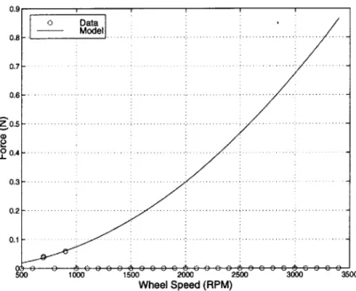
4-9 Setting Analytical Model Parameter, k, Using Ithaco E Wheel Radial Force D ata . . . . 125

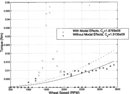
4-10 Setting Analytical Model Parameter, dk, Using Ithaco E Wheel Radial Torque D ata . . . .. .. . . . . 127

4-11 Setting Imbalance Parameters for Analytical Model Using Ithaco E Wheel Data for Fundamental Harmonic . . . . 128

4-12 Setting Damping Parameters for Analytical Model Using Ithaco E Wheel Radial Torque Data for Fundamental Harmonic . . . . 129

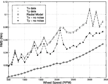
4-13 RMS Comparison of Ithaco E Wheel Radial Torque Data and RWA

distur-bance Models, frequency bandwidth: [0, 1.3Q] . . . .

5-1 Spring Mass Models . . . .

5-2 Coupled spacecraft and RWA system . . . .

5-3 Connection of two components through feedback . . . .

5-4 Example system containing two subsystems . . . .

5-5 Isolated components in free-free form . . . .

5-6 Coupled system for Case #1 . . . .

5-7 Component Models for Case #2 . . . .

5-8 System Model for Case #2 . . . .

5-9 Comparison of Exact Solution and Current Methods Using

Param eters. . . . .

5-10 Representative Reaction Wheel Hard-mounted to Load Cell

Varying Model

5-11 Block Diagram Representation Data Acquisition Configuration for Wheel . 5-12 Full View of Flexible Truss Testbed . . . . 5-13 Representative Reaction Wheel Mounted to Flexible Testbed . . . .

A-1 Coefficient A-2 Coefficient A-3 Coefficient A-4 Coefficient A-5 Coefficient A-6 Coefficient A-7 Coefficient A-8 Coefficient A-9 Coefficient A-10 Coefficient A-11 Coefficient A-12 Coefficient A-13 Coefficient

Curve Fits - Ithaco B Wheel Radial Force (1)

Curve Fits - Ithaco B Wheel Radial Force (2)

Curve Fits - Ithaco B Wheel Radial Force (3)

Curve Fits - Ithaco B Wheel Radial Torque (1)

Curve Fits - Ithaco B Wheel Radial Torque (2)

Curve Fits - Ithaco B Wheel Radial Torque (3)

Curve Fits - Ithaco B Wheel Axial Force . . .

Curve Fits - Ithaco E Wheel Radial Force (1)

Curve Fits - Ithaco E Wheel Radial Force (2)

Curve Fits - Ithaco E Wheel Radial Torque (1)

Curve Fits - Ithaco E Wheel Radial Torque (2)

Curve Fits - Ithaco E Wheel Axial Force (1)

Curve Fits - Ithaco E Wheel Axial Force (2)

C-1 Schematic Diagram of Representative Reaction Wheel Showing Flywheel and

Motor ... ...

C-2 Fitting Plant Transfer Function for Open Loop System . . . . C-3 Block Diagram of Tachometer Control Loop . . . .

C-4 Circuit Diagram of Tachometer Controller . . . . 131 136 137 139 141 141 148 152 152 156 160 160 161 163 173 174 175 176 177 178 179 180 181 182 183 184 185 191 193 193 194

List of Tables

2.1 Frequencies and Amplitudes of X(t) . . . .

2.2 Ithaco TORQWHEEL Design Specifications . . . .

2.3 Frequencies of Ithaco Structural Wheel Modes . . . . .

3.1 3.2 3.3 3.4 3.5 3.6 3.7 3.8 3.9 4.1 4.2 5.1 5.2 5.3 5.4

Ithaco B Wheel F, Data Set . . . .

Bin Statistics for Ithaco B Wheel Radial Harmonics(fLim

Empirical Model Parameters for Ithaco B Wheel . . . .

Empirical Model Parameters for Ithaco E Wheel . . . .

Inputs for Ithaco E Wheel Radial Force Modeling . . . .

Disturbance Amplification in Radial Force Harmonics Disturbance Amplification in Radial Torque Harmonics

Inputs for Ithaco E Wheel Axial Force Modeling . . . .

Disturbance Amplification in Axial Force Harmonics . . Model Parameters and Fitting Methodologies . . . .

Parameters for Analytical Model of Ithaco E Wheel . .

Plant M odels . . . . Compliance conditions for RWA Disturbance Models . . RWA/Spacecraft Coupling Analysis . . . . Summary of Results . . . . . . . . . . . . = 200 Hz) . . . . 31 33 40 49 54 66 74 75 77 83 86 87 . . . . 121 . . . . 130 . . . . 146 . . . . 146 . . . . 147 . . . . 162

Nomenclature

DADM Data Analysis and Disturbnace Modeling

EOM equations of motion FEM finite element model

FFT fast Fourier transform

GSFC Goddard Space Flight Center

HST Hubble Space Telescope

JPL Jet Propulsion Laboratory

NGST Next Generation Space Telescope

PSD power spectral density RMS root mean square RWA reaction wheel assembly

SIM Space Interferometry Mission

Symbols A

A, B, C, D

C

Fpeak, Fbin, Fstat

F H I M, m R, r Rx~r) S T U

us

amplitude coefficient (with modal effects) data set

expected value force

harmonic number identification matrics Fourier transform operator

transfer function inertia Lagrangian mass radius autocorrelation

power spectral density torque, kinetic energy position in inertial frame static imbalance

dynamic imbalance potential energy, voltage work

X(t) stochastic process

XYZ ground-fixed reference frame

a acceleration

d distance

c damping coefficent

cO torsional damping coefficient

f

h harmonic number

i harmonic index, V~T

j

k stiffness

ko torsional stiffness

n number of harmonics in model

s Laplace variable

t, T time variables

u position in body-fixed frame

v translational velocity

x, y translational displacement

xyz body-fixed reference frame

transformation matrix

Q wheel speed

a phase angle

o

damping ratio

0,

#,

y mean

generalized coordinate

o7 2 variance

a

W frequency variable (rad/s), natural frequency, angular velocity

CD RWA disturbance frequency

Subscripts and Superscripts

(.)

()* normalized quantity

(.)H Hermitian (complex-conjugate tanspose)

(.)T transpose

()axi indicates axial force disturbance

()h homogeneous solution

(-)ij (i,j) entry of a matrix (.), particular solution

()rad indicates radial force disturbance

()tor indicates radial torque disturbance

Chapter 1

Introduction

1.1

Motivation

NASA's Origins program is a series of missions planned for launch in the early part of

the 2 1st century that is designed to search for Earth-like planets capable of sustaining life

and to answer questions regarding the origin of the universe. The first generation missions include the Space Interferometry Mission (SIM), which is a space-based interferometer with

astrometry and imaging capabilities [1], and the Next-Generation Space Telescope (NGST),

a near-infrared telescope

1.

improvements in angular resolution and image quality and to meet the goals of high

res-olution and high sensitivity imaging and astrometry [2]. The ability of the missions to

accomplish their objectives will depend heavily on their structural dynamic behavior. SIM and NGST pose challenging problems in the areas of structural dynamics and control since both instruments are large flexible, deployed structures with tight pointing stability requirements. The optical elements on SIM must meet positional tolerances on the order of 1 nanometer across the entire 10 meter baseline of the structure to meet astrometry requirements [3], and those on NGST must be aligned within a fraction of

a wavelength to meet optimal observation requirements [4]. Disturbances from both the

orbital environment (atmospheric drag, gravity gradient, thermal "snap" [5], solar pressure), and on-board mechanical systems and sensors (reaction wheels, optical delay lines, cryo-coolers, mirror drive motors, tape recorders) are expected to impinge on the structure

1

causing vibrations which can introduce jitter in the optical train exceeding the performance requirements. It is expected that the largest disturbances will be generated on-board and will be dominated by vibrations from the reaction wheel assembly (RWA) [3].

1.2

Reaction Wheel Assembly

When maneuvering on orbit, spacecraft generally require an external force, or torque, which is sometimes provided by thrusters. As an alternative, RWA can counteract zero-mean torques on the spacecraft without the consumption of precious fuel and can store momentum induced by very low frequency or DC torques. [6]. They are often used for both spacecraft attitude control [7] and performing large angle slewing maneuvers [8]. Other applications include vibration compensation and orientation control of solar arrays [9]. A typical RWA consists of a rotating flywheel suspended on ball bearings encased in a housing and driven

by an internal brushless DC motor. Ithaco type B and E Wheels are shown in Figures 1-1

and 1-22. The Ithaco B Wheel is the larger of the two wheels pictured in Figure 1-1(a). The smaller wheel is the Ithaco type A wheel and is not discussed in this thesis. The cross-sectional views show that the flywheel is designed such that its mass is concentrated on the outer edges to provide maximum inertia for minimum mass. Alternative RWA designs include the use of magnetic bearings to replace traditional ball bearings [10, 11].

During the manufacturing process, RWAs are balanced to minimize the vibrations that occur during operation. However, it has been found that the vibration forces and torques emitted by the RWA can still degrade the performance of precision instruments in space

[8, 12, 13, 14, 15]. These vibrations generally result from four main sources: flywheel

imbalance, bearing disturbances, motor disturbances and motor driver errors [16]. Flywheel imbalance is generally the largest disturbance source in the RWA and causes a disturbance force and torque at the wheel's spin rate, that is referred to as the fundamental harmonic. There are two types of flywheel imbalances, static and dynamic. Static imbalance results from the offset of the center of mass of the wheel from its spin axis, and dynamic imbalance is caused by the misalignment of the wheel's principle axis and the rotation axis. Bearing disturbances, which are caused by irregularities in the balls, races, and/or cage [17], produce disturbances at both sub- and super-harmonics of the wheel's spin rate. Low frequency

2

(a) External View

Aluminum Aluminum _{Access Panel Bearing Cover}

Housing Flywheel /

I /

Ironless Armature Brushless DC Motor

(b) Cross-Section

(a) External View

Floating Bearing

Pair Ironless Armature

Brushless DC Motor

(b) Cross-Section

disturbances are generally a result of lubricant dynamics, while high frequency disturbances are caused by the bearing irregularities. The torque motor in a RWA is another possible disturbance source. Brushless DC motors exhibit both torque ripple and cogging which generate very high frequency disturbances [16].

1.3

Disturbance Modeling

In general, isolation systems are used to reduce the effects of RWA disturbances on the spacecraft [8, 12, 14, 18]. Models of the disturbances are created for use in disturbance analysis to predict the effects of the vibrations on the spacecraft and allow the development of suitable control and isolation techniques. The most commonly used RWA disturbance model was created to predict the effects of RWA induced vibrations on the Hubble Space Telescope (HST) [15]. The model is based on induced vibration testing performed on the

HST flight wheels and assumes that the disturbances are a series of harmonics at discrete

frequencies with amplitudes proportional to the wheel speed squared. The model is fit to the vibration data and provides a prediction of the disturbances at a given wheel speed. However, during operation it is often necessary to run the RWAs at a range of speeds. Therefore the discrete frequency model was used to create a stochastic broad-band model that predicts the power spectral density (PSD) of RWA disturbances over a given range of wheel speeds [18]. The model assumes that the wheel speed is a random variable with a given probability density function. Both the discrete frequency and stochastic models capture the disturbances of a single RWA. However, in application, multiple RWAs are used to provide multi-axis torques to the spacecraft and for redundancy. Therefore a model was developed which predicts the disturbance PSDs of multiple RWAs in a specified orientation based on a frequency domain disturbance model of a single wheel [4, 19]. The multiple wheel model transforms the RWA disturbances from a frame attached to the RWA to the general spacecraft frame allowing a disturbance analysis.

A performance assessment and enhancement methodology was developed to incorporate

disturbance, sensitivity and uncertainty analyses into a common framework [19]. The ap-proach is presented in block diagram form in Figure 1-3. A disturbance model, generally created from experimental data, d, is used to drive a model of the spacecraft, or plant.

redesign options

d Distutace W + design

disturbance closedl orp) performance margin

data prediction performance

assessment

disturbance plant uncertainty _uncertty

Figure 1-3: Performance Assessment and Enhancement Framework

spacecraft/controller design. The accuracy of the results obtained from this methodology depends heavily on the quality of the disturbance model. If the disturbances are modeled

incorrectly the performance output, z, will not correctly predict the performance of the

spacecraft when exposed to the disturbance environment. Therefore, in order to meet the stringent performance requirements on next generation telescopes, such as SIM and NGST, accurate disturbance models are necessary. Thus, the focus of this thesis is the development of RWA disturbance models for incorporation into the overall performance assessment and enhancement framework and is represented by the shaded block in Figure 1-3.

1.4

Thesis Overview

Figure 1-4 provides a detailed view of the disturbance model block in Figure 1-3. The input,

d, represents RWA vibration data that is used to develop a model, w, for a given wheel.

The five blocks within the dashed line represent the RWA disturbance models that can be used for disturbance analysis. The first block, labeled "Empirical", is based on the discrete frequency HST model. The empirical model extends the HST model for application to any RWA through the development of a MATLAB toolbox that extracts the model parameters from steady-state RWA disturbance data. The empirical model can be represented in either the time or the frequency domain, and can be directly input to the multi-wheel model to predict the disturbances of multiple wheels or can be combined with other models as shown in Figure 1-4. The empirical model alone only captures the disturbances at discrete wheel speeds. In order to predict the broadband behavior of the wheels over a range of speeds

the empirical model parameters are input to the stochastic model (block (e)) to produce a disturbance PSD that can be input to the multi-wheel model. The form of the broadband model also allows easy transformation from PSDs (frequency domain) to state space models

[19].

A second drawback of the empirical model is that it does not capture the internal

flexibility of the RWA. Therefore, it can be combined with an analytical model (block (d)) to produce a more complete extended model (block (f)). The analytical model is the second model discussed in this thesis and captures the physical behavior of an unbalanced rotating flywheel. The model is developed using principles from rotor dynamics and accounts for the structural modes of the RWA which cause disturbance amplification in the vibration data that are not captured by the empirical model.

Although the analytical model captures the internal flexibility of the wheel it is not a complete disturbance model because only the fundamental harmonic is included. Therefore, the analytical and empirical model are combined to create the third model, the extended model. Both the analytical and extended model can be represented in either time or fre-quency domain. Although the models are nonlinear, they can be linearized to obtain time-variant state-space models at discrete wheel speeds. When left in their nonlinear form, the models can be used to explore the transient disturbance behavior of the RWA as it sweeps through wheel speeds.

Both models can be input to the multi-wheel model to produce a disturbance model that can be used in a disturbance analysis. The extended model is the most complete RWA model available, but it is also the most costly to create. Parameter extraction from disturbance data must be performed to obtain both the empirical and analytical model parameters. Therefore, during early stages of design, the use of either the empirical or analytical model may provide a good approximation to the disturbance behavior of the RWA.

The flexibilities of the spacecraft and RWA result in dynamic coupling between the two systems that is not captured in the models discussed above. Therefore it may be necessary to include a final coupling block in Figure 1-4 before the multi-wheel model or between the

multi-wheel model and the disturbance, w. This additional block would incorporate the

effects of dynamic coupling between the RWA and the spacecraft increasing the accuracy of the disturbance models.

subject of Chapter 2. Methods of processing the time domain data are discussed and the details of vibration tests performed on wheels manufactured by Ithaco Space Systems are presented. The empirical model is presented in Chapter 3. The toolbox functions that were developed to extract the model parameters from the steady-state data are discussed in detail, and the vibration data from the Ithaco wheels is used to validate the model. The subjects of Chapter 4 are the analytical and extended models. The development of the models are presented and a parameter matching methodology that fits the analytical model parameters to RWA disturbance data is developed. The Ithaco E Wheel is used to validate the analytical model through comparison with data and the empirical model. Chapter 5 discusses the coupling of a RWA disturbance model to a spacecraft model. Preliminary analyses of the coupling effects and a testing plan for development and validation of a coupling model are presented. In the final chapter of the thesis, Chapter 6, the work is summarized and recommendations are made for future work.

Empirical Stochastic Multi-Wheel w Specifications D a (M)o .itrac Exteded Comments (a) from isolated vibration tests. generally steady-state.

Chapter 2

(b) physical wheel parameters

from manufacturer.

(c) from RWA DADM toolbox.

wheel harmonic only. steady-state model. discrete wheel speeds.

Chapter 3

(d) physical model.

fundamental harmonic and structural wheel modes. steady-state or transient

Chapter 4

(e) assumes wheel speed is a random variable.

broadband disturbances over range of speeds.

by J. Melody

(f) combines empirical and

analytical models. all harmonics and structural wheel modes steady-state or transient

Chapter 4

(g) multiple wheel model.

n wheels at specified orientations.

spacecraft reference frame

by H. Gutierrez

Figure 1-4: RWA Disturbance Models

Chapter 2

RWA Vibration Testing

RWA vibration data are used throughout this thesis to illustrate modeling and parameter matching methodologies and to validate the disturbance models. Both the form and param-eters of the empirical model are based solely on vibration data, and the analytical model parameters are determined using such data. The data are obtained from isolated tests in which the RWA is hardmounted to a fairly rigid test fixture and either spun at discrete

speeds or allowed to spin through a range of speeds. Time histories of the disturbances that result are obtain through load cells mounted at the interface of the wheel and the test fixture. Spectral analysis techniques are used to process the time histories into frequency domain data and gain insight into the nature of RWA disturbances through examination of their frequency content.

The data that will be used for model validation were obtained from wheels manufac-tured by Ithaco Space Systems and tested at Orbital Sciences Corp. and NASA Goddard Space Flight Center (GSFC). This chapter begins with a discussion of the spectral analysis techniques used to process the data. Then, the details of the RWA vibration tests performed

by Orbital and GSFC, and the data that were obtained, are presented. It will be shown

that the data contain disturbance amplifications resulting from flexibility within the wheel. The chapter concludes with a discussion of the structural dynamics of the wheel and its dominant vibration modes.

2.1

Spectral Analysis

In general, a signal can be characterized as either purely deterministic or stochastic (ran-dom). A deterministic signal is one that is exactly predictable over the time period of

interest, such as x(t) = 10sin(27rt). A stochastic signal, on the other hand, is one that

has some random element associated with it. One example of a stochastic process is a sine

wave with random phase: X(t) = 10 sin(27rt + a) where a is evenly distributed between 0

and 27r

[201.

or non-deterministic. The example, X(t), given above is a deterministic stochastic process because it is deterministic in form, but has some random element. Pure white noise, on the other hand, is a nondeterministic stochastic process, since it is purely determined by chance and has no particular structure at all.

RWA disturbances are generally modeled as deterministic random processes similar to the second example given above. Such a process can be characterized by its autocorrelation function, which describes how well the process is correlated with itself at two different times and is defined as:

Rx(r) = Rx (t, t + r) = E[X(t)X(t + r)] (2.1)

where X(t) is a stationary random process and E[-] is the expectation operator. A random process is described as stationary if its probability density functions are time invariant. The autocorrelation function contains information about the frequency content of the process.

If Rx(r) decreases rapidly with time, then the process changes rapidly with time, and

conversely if Rx(T) decreases slowly with time, the process is changing slowly [20]. Taking the Fourier transform of Equation 2.1 produces the power spectral density function, Sx (w)

and transforms the time domain signal to the frequency domain:

Sx(w) = [Rx(T)]

= Rx()ei-idr (2.2)

where F[.] indicates Fourier transform. Conversely, the autocorrelation can be recovered from the spectral density:

1 +Co

1

-- Sx(w)ewrdw (2.3)

Note that the factor - appears in the definition of the inverse Fourier transform. There

is an alternative definition that includes this factor in the Fourier transform [21]. Both definitions are correct and will yield the same results if used consistently. The power spectral density (PSD) provides information about the frequency content of the random signal, and is generally plotted versus frequency.

Another useful frequency domain representation of a stochastic process is the amplitude spectrum. It provides an estimate of the signal amplitude as a function of frequency and is defined as:

1T

Ax(w) =27rT J X(t)eiwtdt (2.4)

where T is the length of the time history. The units of Ax(w) are the same as those of

X(t). If the random signal is X(t) = Ai sin(wot + a) the value of the amplitude spectrum

at the frequency of the sinusoid is equal to the amplitude of the sinusoid: Ax(wo) = A1.

In engineering practice both the power spectral density and the amplitude spectrum are generally plotted against a frequency axis in units of hertz (Hz). Therefore the following transformations are made:

Sx(f) 27rSx(w) (2.5)

Ax(f) 27rAx (w) (2.6)

where Sx

(f)

(f)

have units of X(t)2/Hz and x(t), respectively.

2.1.1 Root Mean Square

The mean, px(t), and variance, ux(t) of a random process, X(t), are defined as

PX(t)= E [X(t)] (2.7)

The mean square, ri is defined as the expected value of the square of the random process and can be expressed in terms of the mean and variance through Equation 2.8:

r2= E [X(t)2]

= 2 + pX (2.9)

The square root of the mean square is referred to as the root mean square (RMS) and is a useful metric for validating the disturbance models through data comparison. It is easy to see from Equation 2.9 that for a zero-mean process the RMS is simply equal to the square root of the variance. For simplicity, the assumption is made that all stochastic disturbances presented in this thesis are zero-mean.

The mean square can also be obtained from the autocorrelation function. Evaluating Equation 2.1 at -r = 0 and using the relationship in Equation 2.9 results in:

Rx(O) = E [X(t)2] = (2.10)

An alternative definition for Rx (0) can be obtained by substituting r = 0 into Equation 2.3

and transforming Sx(w) to Sx(f):

Rx(0) J Sx(f)df (2.11)

Equations 2.10 and 2.11 suggest a relationship between the variance of a random process and its PSD:

+oo

i

J

Therefore, the RMS of a zero-mean, stationary process is simply the square root of the area under the PSD over the frequency band of interest. Equation 2.12 is a powerful result and is used extensively throughout the RWA disturbance modeling and validation processes.

Another metric that is useful in the model validation process is the cumulative RMS, 0xc(fo). It is defined as:

(+fO 2

0-xc

(2f

frmin)

where fo E [fmin, fmax] and fmin and fma are the upper and lower limits of the frequency

Table 2.1: Frequencies and Amplitudes of X(t)

Harmonic Frequency (Hz) Amplitude (N)

1 10 1

2 25 1.5

3 40 4

PSD. In practice, the cumulative RMS of a signal is calculated by dividing its PSD into

smaller segments. The RMS of each of these PSD segments is calculated by integrating over the frequency bandwidth of each segment to obtain the variance of the segment. A running total of the segment variances is computed, and the cumulative RMS is the square root of this total. The cumulative RMS curve is most useful when plotted with the corresponding

PSD or amplitude spectra of the signal. It allows identification of the frequencies at which

significant contributions to the total RMS occur.

2.1.2 Example

A simple example is used to illustrate the concepts presented above and demonstrate their

application. Consider a random process, X(t), that consists of three harmonics:

3

X(t) = Ai sin(wit + ai) (2.14)

i=1

where Ai is the amplitude of the ith harmonic in Newtons (N), wi is the frequency in rad/s,

and ai is a random phase uniformly distributed between 0 and 27r. The signal frequencies and amplitudes used for this example are listed in Table 2.1. The time history of the signal is created in MATLAB using a time vector of length 2048 with a resolution of .01 seconds. This time spacing corresponds to a sampling rate of 100 Hz. A portion of the resulting signal is shown in Figure 2-1(a). It is difficult to determine the frequencies and amplitudes of the sinusoids that generated this signal from the time history. Therefore the signal is transformed to the frequency domain using Equations 2.2 and 2.4.

The resulting amplitude spectra and PSD are plotted in Figure 2-1(b). In this form the frequency content of the signal is obvious. Both functions consist of peaks at the frequencies listed in Table 2.1. Note that the magnitudes of the peaks in Ax correspond to the magnitudes of the sinusoids at each of the frequencies. The magnitudes of the peaks in the PSD, Sx, on the other hand, do not directly present any information about the

0 5 10 20 25 30 35 40 45 so

U)2

--0 0.1 0.2 0.3 0.4 0 5 0.6 0.7 0.8 0.9 1 0 5 10 10 20 20 30 35 40 40 0

Time (s) Frequency (Hz)

(a) Time Domain (b) Frequency Domain

Figure 2-1: Time and Frequency Domain Representations of Stochastic Process, X(t)

amplitudes of X(t). The PSD does however, allow calculation of the RMS of the signal through integration. The bottom plot in Figure 2-1(b) is the cumulative RMS of the signal. Note that the curve is a series of "steps" and that each step occurs at one of the frequencies listed in Table 2.1. Also note that the largest step is at 40 Hz, which is the frequency of the sinusoid with the greatest amplitude. The cumulative RMS can be used in this manner to identify the dominant frequencies in a signal. The final value of the cumulative RMS in this example is 3.1024 N. This value also results from taking the square root of the area under the PSD and is the total RMS of the signal.

2.2

Ithaco RWA Disturbance Data

RWA vibration data from two types of wheels manufactured by Ithaco Space Systems are used in this thesis to illustrate the parameter extraction methodologies for both the empirical and analytical model and to validate the models through data comparison. The wheels that were tested are type B and E Ithaco TORQWHEELs, with model numbers TW-16B32 and TW-50E300. In both cases the wheels were off-the shelf standard catalog products that had not yet been balanced for minimum vibration operation. Pictures of typical Ithaco B and E wheels are shown in Figures 1-1 and 1-2 and the design specifications for the models that were tested are listed in Table 2.2. Notice that the Ithaco E Wheel can

Table 2.2: Ithaco TORQWHEEL Design Specifications Model Number TW-16B32 TW-50E300 Speed Range (rpm) ±5100 +3850 Momentum Capacity (N-m-s) > 16.6 > 50 Reaction Torque (mN-m) > 32.0 > 300 Tachometer (Pulses/Rev) 72 72 Static Imbalance (g.cm) < 1.5 < 1.8 Dynamic Imbalance (g.cm2) < 40 < 60 Peak Power (W) < 50.0 < 280

Mass Reaction Wheel (kg) < 5.9 < 10.6

Mass Motor Driver (kg) included < 3.3

Wheel Diameter (cm) < 25.5 < 39.3

Wheel Height (cm) < 9.3 < 16.6

Motor Driver (cm) included < 21x18x9

provide a significantly greater reaction torque than the Ithaco B Wheel. However, it is also a much larger and much heavier wheel. Both the pictures and the information listed in the table were obtained from the Ithaco Space Systems website (www.ithaco.com).

2.2.1 B Wheel

An Ithaco B Wheel, model TW-16B32, was tested at Orbital Sciences Corp. in German-town, MD in February and April of 1997. Vibration tests were run on two wheels, an engineering and a flight unit for the FUSE mission. Only the data from the flight unit will be presented in this thesis. Vibration data were obtained from a Kistler 9253A force/torque table, which is a steel plate containing four 3-axis load cells. The table was mounted directly to a large granite block that sat upon foam rubber pads. The reaction wheel was mounted to the Kistler table such that the z-axis of the table corresponded to the spin axis of the wheel. The output signals of the load cells were combined to derive the six disturbance forces and torques at the mounting interface between the wheel and the table. Data were taken for approximately 8 seconds once the wheel had reached steady-state spin at every

100 rpm from 500 to 3400. A sampling rate of 1kHz was used, and anti-aliasing filters were

set at 480 Hz. In addition, data was taken with the wheel actively controlled to 0 rpm to provide a measure of sensor and electrical noise.

The data were processed using MATLAB to obtain PSDs and amplitude spectra of the time histories of the wheel disturbances at each speed and the noise data. Figure

2-U- c N M 100 I -10, Frequency (Hz) Frequency (Hz)

(a) Forces (b) Torques

Figure 2-2: Comparison of Noise and Disturbance Data (at 500 rpm) for Ithaco B Wheel (FUSE Flight Unit)

2 compares the noise data to the disturbance data taken at the lowest wheel speed (500

rpm). The three forces, F2, Fy and Fz are shown in Figure 2-2(a) and the three torques,

T, T. and Tz are shown in Figure 2-2(b) Note that in general, the noise data is well

below the disturbance data at frequencies greater than 10 Hz. The only case for which this observation is not true is the Tz data. This torque is the axial disturbance torque and is negligible. Therefore, the Tz disturbance lies very close to the noise floor. Since the wheel disturbances increase as the wheel speed increases, it can be concluded that the noise floor has a negligible effect on the five significant disturbances, F, Fy, Fz, Tz, and Ty.

Frequency domain data can be plotted side-by-side in a 3-dimensional plot called a waterfall plot. Plotting the data in this form allows the identification of disturbance trends across both frequency and wheel speed. An example of a waterfall plot is shown in Figure 2-3(a). The data shown are the Ithaco B Wheel F2, or radial force, disturbances. Note that the dominant disturbances appear as ridges at around 300 Hz and 460 Hz. These disturbances are independent of wheel speed and occur at frequencies corresponding to the resonances of the test fixture. Since these effects are caused by amplification of wheel harmonics by the test fixture dynamics they should not be included in a disturbance model. The second plot, Figure 2-3(b), shows the same data plotted to 200 Hz. Note that now diagonal ridges of disturbances are visible in the data. The frequencies of these disturbances are linearly

0.04 30, - 0.035, z -0.02, 1s,-s 0.01 3 2 0 0 0 0 o0 S oS 2 0 0 01 5 200 s100 200 002 00 15 100 s 1000 100 1000 50

Wheel Speed (RPM) Frequency (Hz) Wheel Speed (RPM) Frequency (Hz)

(a) All Frequencies: Test Stand Mode (b) Truncated: Harmonic Disturbances

Figure 2-3: Waterfall Plot of Ithaco B Wheel F Disturbance Data

dependent on the wheel speed. As the speed of the wheel increases the disturbances slide along the frequency axis. These disturbances are the wheel harmonics that were introduced in Section 1.2. The largest ridge visible in this plot is the fundamental harmonic. Recall that the fundamental harmonic corresponds to disturbances that occur once per revolution and is caused by static and dynamic imbalance of the flywheel. Also note that smaller diagonal ridges are visible. These are super-harmonics caused by bearing imperfections and other disturbance sources within the wheel.

Waterfall plots of all six Ithaco B Wheel disturbance PSDs are presented in Figure 2-4. The signals are truncated at 200 Hz to remove the effects of the test stand resonance and the z-axis on all the plots is kept at the same scale to allow comparison among the directions. The F, and F, data are both radial force disturbances and differ only by 90' of phase. The PSD contains no phase information so, since the RWA is axi-symmetric, the data from these two disturbance directions are nearly identical. Figures 2-4(c) and 2-4(d) are the radial torque disturbances, T and T.. These disturbances are also identical due to the symmetry of the wheel. The final two sub-figures, Figure 2-4(e) and 2-4(f) are the axial force and torque disturbances, respectively. Note that all of the disturbances in the Fz data are amplified around 70 Hz. The source of these amplifications will be discussed in Section 2.3. Also it is clear from Figure 2-4(f) that the axial torques are insignificant in comparison to the other disturbances. The waterfall plot supports the earlier claim that disturbance torques in this direction can be neglected.

2000 ISO 2000

160100 1500 100

1000

~0

Wheel Speed (RPM) Frequency (Hz) Wheel Speed (RPM) Frequency (Hz)

(a) Radial Force, x-direction (b) Radial Force, y-direction

2520

000

150 Wheel Speed (RPM) 500 0 Frequency kHz)

(c) Radial Torque, x-direction

0.04 0.025-.03 a - 0.0s-0.01 0.005,

Wheel Speed (RPM) Frequency (Hz)

(e) Axial Force, z-direction

250o

2000 150

150 10

Wheel Speed (RPM) 500 Frequency (Hz)

(d) Radial Torque, y-direction

2500

boo 10 0

Wheel Speed (RPM) 500 0 Frequency (Hz)

(f) Axial Torque, z-direction

Figure 2-4: RWA Disturbance Data - Ithaco B Wheel

200

2.2.2

E Wheel

An Ithaco E Wheel, model TW-50E300 was tested at the NASA Goddard Space Flight

Center (GSFC). The wheel was integrated into a stiff cylindrical test fixture and hard-mounted to a 6-axis Kistler force/torque table. In this test, the wheel was started at 0 rpm and full torque voltage was applied to the motor until the wheel saturated around 2400 rpm. The data was sampled at 3840 Hz for 390 seconds and 8 channels of load cell data were obtained. These channels were combined to derive the disturbance forces and torques at the mounting interface between the wheel and the table. Note that this vibration test was not conducted at steady-state speeds like the Ithaco B Wheel test performed at Orbital. Therefore, in order to use the data to obtain a steady-state empirical model, a technique was developed to obtain steady-state frequency domain data from the continuous time histories.

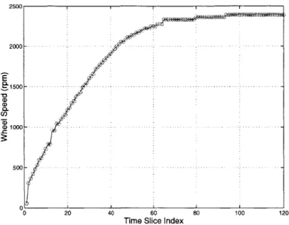
The spin-up of the wheel occurred at a relatively slow rate, so the resulting time history can be subdivided into time slices that are considered to be quasi-steady state. Each time slice has a sample length of 2.133 seconds and contains 8192 points. These time histories are then transformed to the frequency domain through the PSD and amplitude spectra. The frequency content of the signal is used to determine the average wheel speed of each time slice by assuming that the fundamental harmonic causes the most significant disturbance. Based on this assumption, the frequency at which the maximum disturbance occurs in a given time slice is also the average speed of the wheel. In Figure 2-5 the average wheel speeds are plotted versus the time slice number. The data were processed into 120 time slices, and the curve indicates that the assumption used to identify the wheel speeds is a valid one. As the time slice index increases the wheel speed also increases until the wheel saturates around 2400 rpm [22].

When processed as described above, the Ithaco E Wheel data can be treated as steady-state data similar to the Ithaco B Wheel data. The waterfall plots of the six disturbance PSDs are shown in Figure 2-6. The test fixture that the Ithaco E Wheel was mounted to is stiffer than that used for the Ithaco B Wheel. Therefore, the data are not corrupted by test stand resonances and can be plotted up to 300 Hz. The orientation of the wheel was such that F, and F are the radial forces, T and T. are the radial torques, and Fz and Tz are the axial forces and torques, respectively. The fundamental harmonic is clearly visible in the

0 20 40 60 80 100 120

Time Slice Index

Figure 2-5: Wheel Speeds Corresponding to Quasi-Steady State Time Slices

radial forces and torques and the axial force. The two radial force plots, Figures 6(a) and

2-6(b), show that the number and shape of the harmonics visible in these disturbances are

similar. The same observation can be made with regard to the radial torques, Figures 2-6(c) and 2-6(d). Also note that, like the Ithaco B Wheel data, the axial torque (Figure 2-6(f)) is negligible when compared to the other disturbances. Finally, similar to the Ithaco B Wheel Fz data, there are regions of disturbance amplification visible at low frequencies in all five of the Ithaco E Wheel disturbances. Since the test stand resonance was greater than 300 Hz for this test, another explanation for the amplifications must be found. These resonant effects are the subject of the following section.

2.3

Structural Wheel Modes

The RWA can be modeled as having five degrees of freedom, translation in the axial direc-tion, translation in the two radial directions and rotation about the two radial axes. This model results in three dominant vibration modes: axial translation, radial translation and radial rocking. These modes are depicted schematically in Figure 2-7. The natural frequen-cies of the three modes reported by Ithaco for type B and E TORQWHEELS are listed in Table 2.3 [16]. The radial rocking mode consists of two whirl modes, the positive whirl and the negative whirl, which have natural frequencies that are dependent on the speed of

0.04, 0.035 - 0.03,- 0.025,-Z0.02, 00.015,-0.01 0.005 0, 2000 1500 1000

Wheel Speed (RPM) Wheel Speed (RPM)

(a) Radial Force, x-direction

0.04. 0.035, 0.03, 0.025, E 0.02. 0.015, C. 0.01. 0.005. 1500 1000 0 Wheel Speed (RPM) 1002 Frequency (Hz)

(c) Radial Torque, x-direction

Wheel Speed (RPM)

(b) Radial Force, y-direction

250

0 0

100

Frequency (Hz)

(d) Radial Torque, y-direction

0.04, 0.035 --0.03, N 0.025, E 0.02, z 0.015, C. 0.01. 0.005. 1500 1000 500 Wheel Speed (RPM) 50 100F Frequency (Hz) 1000 500 Wheel Speed (RPM) 150 200 50 Frequency (Hz)

(e) Axial Force, z-direction (f) Axial Torque, z-direction

Figure 2-6: RWA Disturbance Data -Ithaco E Wheel

0.04-0.035, 0.03,- 0.025,-Z 0.02-0.015, 0.01 --0.005, 250 200 100F Frequency (Hz) 1500 250 0 0 100 Frequency (Hz) 0.04. 0.035,. 0.03. N 0.025, E 0.02. 0.015, CL 0.01. 0.005. 0. 0.04. 0.035. 0.03,. 10.025. Z 0.02. 00.015. 0.01. 0.005. 0-2000 300 1000 2000 1500