An iterative study of time independent induction effects in magnetohydrodynamics

HAL Id: hal-00492367

https://hal.archives-ouvertes.fr/hal-00492367

Submitted on 15 Jun 2010

HAL is a multi-disciplinary open access

archive for the deposit and dissemination of

sci-entific research documents, whether they are

pub-lished or not. The documents may come from

teaching and research institutions in France or

abroad, or from public or private research centers.

L’archive ouverte pluridisciplinaire HAL, est

destinée au dépôt et à la diffusion de documents

scientifiques de niveau recherche, publiés ou non,

émanant des établissements d’enseignement et de

recherche français ou étrangers, des laboratoires

publics ou privés.

An iterative study of time independent induction effects

in magnetohydrodynamics

Mickaël Bourgoin, Philippe Odier, Jean-François Pinton, Yanick Ricard

To cite this version:

Mickaël Bourgoin, Philippe Odier, Jean-François Pinton, Yanick Ricard. An iterative study of time

independent induction effects in magnetohydrodynamics. Physics of Fluids, American Institute of

Physics, 2004, 16 (7), pp.2529-2547. �10.1063/1.1739401�. �hal-00492367�

An iterative study of time independent induction effects

in magnetohydrodynamics

M. Bourgoin, P. Odier, and J.-F. Pintona)

Laboratoire de Physique, CNRS UMR#5672, E´ cole Normale Supe´rieure de Lyon, 46 alle´e d’Italie, F-69007 Lyon, France

Y. Ricard

Laboratoire des Sciences de la Terre, CNRS UMR#5570, E´ cole Normale Supe´rieure de Lyon, 46 alle´e d’Italie, F-69007 Lyon, France

共Received 31 October 2003; accepted 23 March 2004; published online 2 June 2004兲

We introduce a new numerical approach to study magnetic induction in flows of an electrically conducting fluid submitted to an external applied field B0. In our procedure the induction equation

is solved iteratively in successive orders of the magnetic Reynolds number Rm. All electrical quantities such as potential, currents, and fields are computed explicitly with real boundary conditions. We validate our approach on the well known case of the expulsion of magnetic field lines from large scale eddies. We then apply our technique to the study of the induction mechanisms in the von Ka´rma´n flows generated in the gap between coaxial rotating disks. We demonstrate how the omega and alpha effects develop in this flow, and how they could cooperate to generate a dynamo in this homogeneous geometry. We also discuss induction effects that specifically result from boundary conditions. © 2004 American Institute of Physics. 关DOI: 10.1063/1.1739401兴

I. INTRODUCTION

When a magnetic field is applied to a flow of an electri-cally conducting fluid, complex induction mechanisms occur and induced currents and magnetic field are generated. For certain particular flows, this induction process may generate an instability where the induced magnetic field adds up to the initial one such that a large-scale field can grow. This phe-nomenon, known as the magnetohydrodynamic 共MHD兲 dy-namo instability, is thought to be the source of cosmic bod-ies’ magnetic fields, as originally suggested by Larmor in 1919.1

Experimentally, dynamo action has first been produced by the controlled motion of solid metal rotors. The setup designed by Lowes and Wilkinson2uses two metal cylinders with their axis at an angle. The differential rotation generated by each rotating cylinder inside a stationary conductor con-verts a poloidal field into an azimuthal one. A loop-back instability mechanism is created because the azimuthal in-duced field proin-duced by each cylinder plays the role of an axial field for the other rotating conductor. Fluid dynamos have also been demonstrated experimentally by the Karlsruhe and Riga experiments.3,4 These experiments have been built so that the mean fluid flow mimics model 共lami-nar兲 configurations where dynamo action has been analyti-cally calculated.5,6 In each case, observations have shown that the experimental dynamo onset is very close to that cal-culated from the laminar mean flow alone.7,8 In order to study the backreaction and the time dynamics of fluid dyna-mos above threshold, it would be desirable to build less

con-strained flows that are capable of self-generation. In this quest, several groups have focused on swirling flows gener-ated by the rotation of coaxial impellers in a closed volume.9 These flows possess differential rotation and helicity, two ingredients that play a central role in dynamo self-generation.10Kinematic simulations have shown that dy-namo action is a possibility in these flows,11,12but a dynamo loop-back mechanism has been clearly identified, as it was for instance for the Lowes and Wilkinson dynamo.

The understanding of this mechanism is of crucial im-portance for experimentalists. Indeed, kinematic simulations show that for any experimental configuration, the critical value for the control parameter共magnetic Reynolds number, Rm, see next section兲 is always very close to the maximum value achievable in the experiment. If one wants to increase the magnetic Reynolds number, a strong limiting factor is the cost in power consumption P of the engines driving the flow which scales like Rm3.15,19The success of an experimental dynamo relies therefore on a proper identification of the loop-back mechanism and of the geometry of the magnetic field and electrical currents in the experimental vessel to op-timize the design of the experiment.

The purpose of this paper is to study in detail the induc-tion mechanisms that occur in von Ka´rma´n 共VK兲 swirling flows, generated inside a cylinder by the rotation of one or two coaxial disks. However, the method could be easily ex-tended to other types of geometries, some of which more appropriate for geophysical applications.

We consider the induced magnetic and electrical re-sponse of the flow when an external field is applied. Tradi-tional techniques to solve the equation governing the behav-ior of the magnetic field in a fluid 关Eq. 共1兲, Sec. II A兴 use a decomposition on special functions and express boundary a兲_{Author to whom correspondence should be addressed. Electronic mail:}

pinton@ens-lyon.fr

PHYSICS OF FLUIDS VOLUME 16, NUMBER 7 JULY 2004

2529

conditions as nonlocal spectral conditions, therefore only al-lowing the treatment of simple boundary geometries, such as spherical or cylindrical vessels. We propose here a quasi-static perturbative approach in which complex boundary con-ditions 共close to experimental reality兲 can be conveniently implemented. The net magnetic induction is expressed as the result of an iterative process where the flow subjected to a given field of order Bkinduces the next order Bk_⫹1. For each

iterative step we compute all electromagnetic quantities in-volved in the induction process: induced electromotive force

共e.m.f.兲, currents, and magnetic field. In this approach

suc-cessive iterations correspond to the onset of new couplings as Rm increases. An experimentalist can therefore identify these couplings and understand how they cooperate to favor or hinder the dynamo action and also understand the role of the boundary conditions 共see Figs. 9, 10, and 13兲. This pro-vides a useful guidance for the design and optimization of experiments. Actually, the work described in this paper was originally motivated by the necessity for experimentalists to better understand the path of electrical currents, without which, for instance, the effects related to the boundary con-ditions共see Fig. 13兲 cannot be understood.

The paper is organized as follows: in Sec. II, we present in detail our iterative approach, its links with more tradi-tional kinematic simulations, the implementation of bound-ary conditions and numerical strategies. In Sec. III, we revisit the process of expulsion of magnetic field lines by a large eddy as a test case for the iterative method. We then consider the induction due to differential rotation共Sec. IV兲 and helical motion 共Sec. V兲 in VK flows. In Sec. VI, we discuss the possible generation of an ␣–␻ dynamo in this geometry. Section VII is devoted to the study of an induction mecha-nism in VK geometry that is mainly due to the boundary conditions at the lateral wall of the flow.

II. A QUASISTATIC ITERATIVE APPROACH

Our aim is to describe and understand the induction ef-fects that take place in a stationary flow of an electrically conducting fluid submitted to an external magnetic field, when the magnetic Reynolds number is increased 共Rm is defined as the ratio of induction to Joule dissipation effects兲. The iterative procedure consists in solving step by step the induction equation, and obtain the induced field as a series in Rm. One computes to first order in Rm the magnetic field B1

induced from the applied field B0; the procedure is repeated

to compute the field B2induced from B1at first order, and so

forth. Since the induction equation is linear, the net magnetic field is the sum over all contributions. As we will see, this approach converges strictly only at small Rm, but it can be extended to larger values and the results are in remarkable agreement with experimental data.

A. Induction equation and boundary conditions In the MHD approximation,10the magnetic response of a flow with velocity u共r兲 to an applied uniform field B0 is

governed by

⳵tB⫽ⵜÃ关uÃ共B⫹B0兲兴⫹␭⌬B, 共1兲

“"B⫽0, 共2兲

where␭⫽1/␮0␴ is the fluid magnetic diffusivity共electrical

conductivity ␴兲. The flow velocity u共r兲 is assumed to be stationary. MHD experiments being usually conducted in liq-uid metals, we also assume that the flow is incompressible,

“"u⫽0. We further assume that Lorentz forces remain small

compared to inertial and pressure forces, i.e., the magnetic field never grows strong enough to perturb the prescribed hydrodynamic velocity field—the interaction parameter re-mains small, N⫽␴LB₀2/␳U where ␳ is the fluid’s density, and U, L characteristic velocity and size of the flow. The problem considered here is of the same nature as addressed by kinematic simulations in which the flow is fixed and one studies its magnetic response.

The induction Eq. 共1兲 must be supplemented with boundary conditions. Their choice depends on the definition of the MHD ‘‘system.’’ One simple and elegant solution is to consider the system as being the unbounded space, in which case the condition is that of vanishing magnetic field at in-finity共Dirichlet兲. In this case, the inhomogeneities of electri-cal conductivity are taken into account as an additional term in the induction equation

⳵tB⫽“关uÃ共B⫹B0兲兴⫹␭⌬B⫹共“ÃB兲⫻“␭. 共3兲

This formulation yields a well posed problem, although not practical for numerical implementations. One thus reverts to a finite homogeneous system with specific conditions at the flow walls: in the case of insulating outer walls, Eq. 共1兲 is then supplemented by the condition of continuity of the mag-netic field at the wall共absence of outgoing currents兲. B. The iterative scheme

In order to compute the induced magnetic field for a given applied field, conventional techniques as used in kine-matic simulations would directly solves Eq. 共1兲. This would yield a complete solution, including its time dependence. However, we are interested in understanding how the system reaches a steady-state equilibrium between diffusion and in-duction, a process that we call an ‘‘induction mechanism.’’ We wish to analyze the role of the various components of the velocity field and their gradients, and the role of the bound-ary conditions. We thus develop an approach in which suc-cessive contributions to the net induction共linear in Rm, then quadratic, cubic, etc.兲 are individually identified and their relative importance estimated as Rm is varied.

For a given velocity distribution u共r兲 and applied field B0, we search for steady solutions of the induction equation

B⫽B0⫹Bind, Bind⫽

兺

k⫽1

⬁

Bk, 兩Bk兩⬃O共Rmk兲. 共4兲

In the numerical computation the magnetic Reynolds number Rm is defined as

Rm⫽UL/␭, 共5兲

where U⫽maxr(兩u(r)兩) and L are characteristic integral

ve-locity and length scales of the flow共for example L can be the radius R of the cylinder in VK flows兲. As we look for

sta-tionary solutions, contributions at each order are obtained as solutions of a hierarchy of Poisson equations

⌬Bk⫹1⫽⫺Rm“Ã共uÃBk兲, 共6兲

in which lengths, velocities, and magnetic fields have been nondimensionalized, respectively, by, L, U, and B0.

Each step described by Eq. 共6兲 can be interpreted as usual in terms of distorsion and transport of the magnetic field lines by the velocity gradients of the flow. Even without resolving numerically this set of equations, one has here a way, if the magnetic Reynolds number remains moderate, to picture the mechanisms involved in the induction of mag-netic field, in relation with the main velocity gradients of the flow, as well as a good insight on the spatial structure of the magnetic field.

C. Calculation at each order

Solving Eq.共6兲 by a simple Poisson solver is not trivial as it would imply writing the boundary conditions for the magnetic field at the surface of a cylinder. Instead we start from electric potential and induced currents. The fields at each order are thus considered successively, using the fol-lowing sequence.

共1兲 The electromotive force 共e.m.f. in units of UB0) induced

by the flow motion is computed as

ek_⫹1⫽uÃBk. 共7兲

共2兲 Since the electrical current, given by Ohm’s law j⫽␴共⫺“␾⫹e兲, is divergence free, the electric potential is obtained as a solution the Poisson equation

⌬␾k⫹1⫽“"共uÃBk兲. 共8兲

In the case of an insulating boundary, the condition of vanishing outgoing currents can then be written as n"“␾

⫽n"共uÃB兲. The earlier Poisson equation can then easily

be solved as a von Neuman problem, for any kind of geometry. Note that in real flows the hydrodynamic boundary layer is very small since the magnetic Prandtl number of liquid metals is less than 10⫺5; as a result the viscous sublayer is of negligible extend compared to magnetic scales. A free slip rather than no-slip boundary condition for the velocity is appropriate and the bound-ary condition at the wall, n"“␾is therefore nonzero.

共3兲 The induced currents 共in units of␴UB0) are then

com-puted as

jk⫹1⫽⫺“␾k⫹1⫹ek⫹1. 共9兲

共4兲 Finally, the magnetic field can be computed from Biot–

Savart formula Bk⫹1共r兲⫽ Rm 4␲

冕

_⬘

⬘

⬘

⬘

In practice, the integral is only computed at the boundary and used to provide boundary conditions to solve the Dirichlet problem⌬B_k⫹1⫽Rm“Ãj_k⫹1.

共5兲 The magnetic Reynolds number only enters in the final

step, where all contributions are collected and the fields are obtained as integer series

␾k共Rm兲⫽␾k共1兲Rmk⫺1⇒␾共Rm兲⫽

兺

兺

兺

This approach is valid when the series converges, that is for a low enough value of Rm共Rm⬍Rm*_{兲. Numerically}

we observe that Rm*⬃5–30 in the cases considered in

our study. This range covers a significant fraction of magnetic Reynolds numbers that have been explored in experiments using liquid gallium14,15 and liquid sodium.16,18,19One may also recall that the integral mag-netic Reynolds number 共i.e., defined on large scale physical parameters兲 is an upper limit for the actual mag-netic Reynolds number of the flow 共as a number which actually measures the strength of induction effects兲.20 For higher magnetic Reynolds number values, one needs to extrapolate the series expansion outside its strict con-vergence radius. We use Pade´ approximants,21which has become traditional in these problems共see, for example, Ref. 22兲. It yields strikingly good results when compared to analytical solutions or measurements, as will be shown in the next sections.

D. Numerical implementation

As explained, our study concentrates on the von Ka´rma´n flows, although the approach could be easily applied to other geometries. In experimental configurations, von Ka´rma´n flows are generated inside a cylinder by the rotation of one or two discs whose axis of rotation coincides with the axis of the cylinder. Two regimes are of particular interest.

共1兲 Single disk 共SD兲: a single disk is rotated at frequency ⍀,

the other being held at rest. In this case the time-averaged flow is strongly helical: it has a toroidal com-ponent, and a recirculation poloidal loop, created by the pumping effect towards the center of the rotating disc. In Duddley and James terminology,11it is a s1t1-like flow. 共2兲 Double disk 共DD兲: the disks are counter-rotated at equal

rates⍀. In this case, the mean flow is made of two cells with opposite toroidal velocities and two recirculation loops, with a strong shear zone in-between. Using again Duddley and James terminology,11it is a s2t2-like flow.

In our numerical studies the flow is a synthetic velocity field that mimics the main properties of the experimental mean flows. The aspect ratio of the flow is one, i.e., the height of the cylinder is equal to its diameter 共and will re-main so throughout our study兲. We choose simple harmonic functions for the radial and azimuthal velocities ur and

2531 Phys. Fluids, Vol. 16, No. 7, July 2004 An iterative study of induction effects

u_␪ and deduce the vertical component u_z from the incom-pressibility condition. For the共SD兲 case we use

ur共r,z兲⫽⫺sin␲r cos ␲共z⫹1兲 2 , u_␪共r,z兲⫽2共P/T兲⫺1sin␲r, 共14兲 u_z共r,z兲⫽ 1 ␲rsin ␲共z⫹1兲 2 共␲r cos␲r⫹sin␲r兲,

where (r,␪,z) are the cylindrical polar coordinates, and P/T the ratio of the amplitude of poloidal to toroidal speeds. For the counter-rotating 共DD兲 flow configuration the velocity field is ur共r,z兲⫽⫺sin␲r cos␲z, u_␪共r,z兲⫽2共P/T兲⫺1sin␲z 2 sin␲r, 共15兲 uz共r,z兲⫽ 1

␲rsin␲z共␲r cos␲r⫹sin␲r兲.

In sharp contrast with experimental works,18the flows stud-ied here are smooth and laminar. The effect of turbulent fluc-tuations 共always present in real liquid metal flows at finite Rm兲 cannot be directly computed with this numerical scheme, and other approaches are needed.23

Figure 1共a兲 shows the synthetic flow profile in the 共SD兲 case. One observes poloidal recirculation loops 共arrows兲 as the fluid is drawn to the disk near the axis of the cylinder and ejected towards the lateral wall at the disk outer rim. The toroidal velocity is close to solid body rotation up to r

⯝0.5. The main motion of the flow is helical. The 共DD兲 flow

is shown in Fig. 1共b兲. Two poloidal recirculating loops are now created, since in each half of the cylinder the fluid near the axis is drawn to the closer disk. The toroidal motions are also of opposite directions, so that helicities add up in each half of the cylinder. In addition, there is a strong differential rotation and a shear layer/stagnation point in the middle of the cylinder. In both cases, the velocity boundary condition is that of no outgoing flow, with free slip at the surface. This latter condition is justified because the thickness of the hy-drodynamic boundary layer in liquid metal flows is very small. The ratio P/T of the intensity of the poloidal to toroi-dal velocities is adjustable in the synthetic flows; it is set to 0.8 in the examples shown in Fig. 1, and in most studies here.

Numerically, the crucial part of the scheme lies in the solution of the Poisson equations for the electric potential and for the magnetic field inside the volume. They are then solved using standard programs in the Overture24 library us-ing the mixed Cartesian-cylindrical grid shown in Fig. 1共c兲. In order to reproduce induction effects that do occur in experiments, we have also used in Sec. VII velocity fields obtained by time averaging local velocity measurements in laboratory flows. These fields have been provided by our colleagues at Commissariat a` l’Energie Atomique 共CEA兲 in Saclay, from measurements in a VK flow in water.25

E. Iterative approach and dynamo action

Induction computed with the iterative approach can be linked to dynamo self-generation as follows. Let us rewrite the magnetic field induced at order k⫹1 from the field at order k as

Bk⫹1⫽⫺Rm⌬⫺1关“Ã共uÃBk兲兴⫽Rm G共Bk兲, 共16兲

where we introduce the operatorG:

G•⫽⌬⫺1_{关“Ã共uÕ兲兴. 共17兲}

Let us assume further that an induction loop back mechanism may be identified for a given velocity field and geometry, i.e., that there exists a magnetic field distribution at order k, Bk, such that after n induction iterations, the

resulting magnetic field is similar in geometry with the initial B_k:

B_k⫹n共Rm兲⫽Rmn共G兲n共B_k兲⫽␥RmnB_k, 共18兲 with␥a constant factor that depends on the flow and on the initial magnetic field geometry. At a given magnetic Rey-nolds number the net amplification factor is thus␥Rmn 关i.e.,

␥Rmn and B are eigen value and eigen vector of the opera-tion (G)n]. Positive ␥ values lead to a growth of the mag-netic field mode Bkand thus may lead to a dynamo

instabil-ity if␥Rmn⬎1, the critical magnetic Reynolds number being

Rmc⫽␥⫺n 共19兲

共note again that only stationary dynamos can be captured

using this procedure兲. Negative values of ␥ correspond to processes where the induced magnetic field opposes the ap-plied one. Such situation occur for example in the expulsion of magnetic field lines from eddies26,27—this case will be discussed in detail in Sec. III.

When a positive loop-back mechanism exists, the geom-etry of the marginal mode can also be identified, in much the same manner as in kinematic dynamo studies. Indeed, in kinematic approaches, the neutral mode satisfies

NRmc共B_marginal兲⫽0, 共20兲

with Rmc the critical magnetic Reynolds number, and the operatorN_Rmdefined as

NRm•⫽Rm“Ã共u共r兲Õ兲⫹⌬•. 共21兲

Comparing the definition of the operators G and NRm 关Eqs. 共17兲 and 共21兲兴, Eq. 共20兲 can be interpreted as an n ⫽1 loop-back induction

Bmarginal⫽RmcG共Bmarginal兲⫽Rmc␥Bmarginal, 共22兲

with again the condition Rmc␥⫽1. If the iteration procedure has identified a positive loop-back mechanism in n steps, (B0,B1,...,Bn), one can easily show that there exists a linear

combination Bmarginal⫽⌺k⫽0...n⫺1␭kBk such that GBmarginal ⫽␥Bmarginal 共in fact Bmarginal is an eigenvector of the

sub-space stable under G兲. The neutral mode is thus obtained from the structure of the magnetic field induced at each step in a loop-back mechanism. The occurrence of such processes and its applications to dynamo action in VK flows will be discussed in Sec. VI.

III. COROTATING FLOW: EXPULSION BY LARGE SCALE EDDIES

We first apply the iterative approach to a case that has been well studied analytically28and experimentally:27the ex-pulsion of magnetic field lines by large eddies. To this end, the computational cylinder is divided into a region in solid body rotation (ur⫽uz⫽0, u␪⫽⍀r, up to radius R⫽1)

sur-rounded by a region at rest共up to R⫽2); the medium within the cylinder has uniform electrical conductivity␴and is sur-rounded by insulating material. The cylinder is periodized in

the z direction, so the system is quasi-two-dimensional. An external magnetic field B₀⫽B₀xˆ is applied perpendicular to

the cylinder axis, along the x axis. The solution to this prob-lem can be found analytically.28In cylindrical polar coordi-nates, one has for the stationary state

Br/B0⫽r⫺1兵R关 f共r,p兲cos␪兴⫺I关 f 共r,p兲sin␪兴其,

B_␪/B₀⫽⫺⳵_rI关 f共r,p兲兴, 共23兲

FIG. 1. Flow geometry.共a兲 One rotat-ing disk at the top end of the cylinder (z⫽1): poloidal 共left, arrows兲 and to-roidal共right, gray-scale兲 in the 共SD兲 case; 共b兲 idem for counter-rotating disks;共c兲 numerical grid used for the finite-difference calculations. The co-ordinate system shown is used throughout the text: z is the axis of the cylinder, (x,y ) are transverse and the origin O is set in the middle of the cylinder. The height of the cylinder is equal to its radius共aspect ratio one兲.

2533 Phys. Fluids, Vol. 16, No. 7, July 2004 An iterative study of induction effects

f共p,r兲⫽DJ1共pr兲, r⬍R, f共r,p兲⫽r⫹C/r, r⬎R, 共24兲 p⫽共i⫺1兲

冑

冑

functions兴. Physically, the initially transverse field lines are advected and stretched by the solid body rotation, thus ‘‘be-ing pushed away’’ to the sides of the cylinder while the inner core field decreases under diffusion. From an equivalent point of view, the applied field is time periodic in the refer-ence frame of the rotating core and thus can penetrate only as far as the skin depth␦⫽R/

冑

We now show how this behavior is described by the iterative approach. At first order the induced e.m.f.

e1⫽uÃB0⫽⫺r⍀B0cos␪zˆ⫽⫺x⍀B0zˆ 共26兲

is purely axial and divergence-free. As a result the induced current density j1 has no potential contribution and is

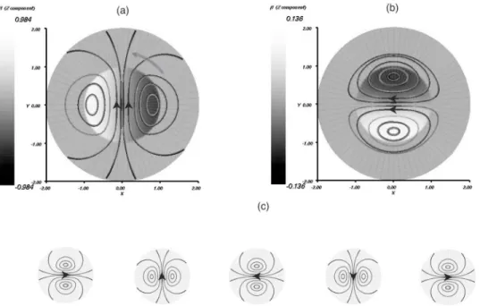
iden-tical to the e.m.f. distribution关see Eq. 共9兲兴. It is thus made of axial currents that flow in opposite directions on each side of the y Oz plane, as shown in Fig. 2共a兲. The resulting induced magnetic field at first order B1has a dipole structure, aligned

with the y axis: the main effect of the rotation is to induce a field component perpendicular to the applied one. The sec-ond order induction just repeats this sequence: as B1 lies in

the (x,y ) plane, the second order electric potential is diver-gence free and the second order currents are j2⫽e2 ⫽uÃB1. They flow axially in opposite direction on either

side of the xOz plane—Fig. 2共b兲. The resulting induced magnetic field is a dipole along the x axis and opposite to B0. This two-step process thus tends to reduce the applied

field, it is the essential mechanism of the expulsion of the magnetic field from the core of the rotating motion—as an illustration, the induction steps 20–24 are displayed in Fig. 2共c兲 showing the stability of the order-two cycle of induction patterns. In fact the two modes, ‘‘x-axis dipole’’ b₁ and ‘‘y-axis dipole’’ b₂, form a stable subspace underG, such that

G共b1兲⫽␥1b2, ␥1⫽1.697⫻10⫺1, 共27兲 G共b2兲⫽␥2b1, ␥2⫽⫺1.697⫻10⫺1, 共28兲 G2_共b

1,2兲⫽␥b1,2, ␥⫽␥1␥2⫽⫺2.879⫻10⫺3. 共29兲

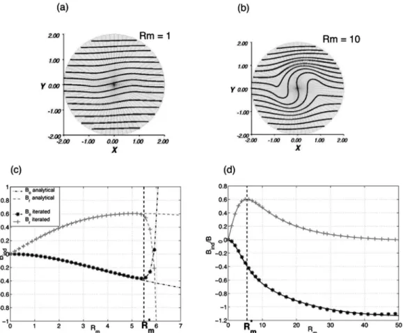
The negative value of␥ leads to the expulsion process. We show in Figs. 3共a兲 and 3共b兲 the profile of magnetic field lines obtains after the iteration of 40 steps. At low magnetic Reynolds number关Rm⫽1 in 共a兲兴 the raw series is computed; in 共b兲 the Reynolds number is equal to 10, larger than the radius of convergence of the series and Pade´ resummation has been used to ensure convergence. The results are in very good agreement with the original numerical calculations by Weiss.26 To be more quantitative, we plot a comparison of the numerical and analytical variations with Rm in Figs. 3共c兲 and 3共d兲. In 共c兲 the raw series up to order 40 is used; the series diverges for Rm⬎Rm*_{⯝5.5, but below the agreement}

is excellent. If Pade´ resummation is applied, as in 共d兲, one gets an excellent agreement at least up to Rm⯝40. Note that the observed radius of convergence of the series is very well approximated by Rm*⫽1/

冑

inferred by starting the iteration process with one of the stables modes (b1,b2): the net induced field is obtained as a

series in powers of ␥1␥2Rm2.

IV. OMEGA EFFECT AND FIELD EXPULSION

In this section we consider the 共DD兲 case of the VK flow, generated when counter-rotation at equal rates is

FIG. 2. Expulsion by rotation.共a兲 First order induction; currents are shown as a gray scale, while the lines give selected magnetic field paths; note that a domain of radius 2R, twice the cylinder size, is represented.共b兲 Idem for second order induction; 共c兲 iteration steps of order 20–24, left to right.

imposed—Fig. 1共b兲. We consider in the section the response of the fluid to an applied field, homogenous and aligned with the cylinder axis 共z direction兲. At low Rm, the differential rotation 共velocity gradients ⳵zu␪) generates an azimuthal

magnetic field, via the␻effect. In the poloidal recirculation loops, the velocity gradients⳵zurand⳵zuz also induce axial

and radial magnetic fields. At high Rm, expulsion occurs and induction decreases.

A. First order induction

In this geometry, experiments14 have shown that the magnetic induction varies linearly with Rm at low Rm, so that first order calculations should give the main features. The first order e.m.f., e₁⫽uÃB₀, gives rise to an electric potential that solves

⌬␾1⫽B0"␻, 共30兲

关from Eq. 共8兲兴 where ␻⫽“Ãu is the vorticity of the flow.

The advantage of this notation is to emphasize the role played by vorticity in the induction process. Note that VK flows have a vorticity field that has the same topological structure as the velocity; in this sense they are very similar to Beltrami flows. Contrarily to the case considered in the pre-vious section, the electric potential must be nonzero to en-sure that currents remain divergence free. Its topology is shown in Fig. 4: it has essential contributions on the cylinder

axis and near the outer rims of the ends of the cylinder. Indeed, on the axis the vorticity is aligned with the applied field, with opposite signs at each end; this leads to the axial potential difference. Near the outer rims of the cylinder, the axial vorticity is reversed compared to that on the axis; it generates in this region a radial potential difference. The in-duced currents result from the potential distribution and local induction j1⫽⫺“␾1⫹e1; their geometry is quite complex,

but two limiting cases can be identified.

共i兲 One case is shown in Fig. 4共a兲. The axial potential

difference drives an axial current 共actually all axial currents are necessarily of potential origin since B0 is axial兲 from one

end of the cylinder to the other. Then currents are transported away from the axis by the induction e.m.f. uÃB0—note that

this is done against the radial potential difference, explaining why the current spirals radially outward 共respectively in-ward兲 in this region. When at the outer wall, the current can again flow axially under the action of the outer axial poten-tial difference. The results is the formation of poloidal cur-rents on a torus, which generate a toroidal magnetic field. This is the␻effect, usually described in terms of torsion of axial magnetic field lines, interpreted here in terms of electric potential and current paths.

共ii兲 Another limiting case corresponds to purely

azi-muthal currents which can only be generated from the induc-tion e.m.f. uÃB₀ since the flow is axisymmetric. In the

me-FIG. 3. Expulsion by rotation.共a兲 and 共b兲 Magnetic field lines computed using the iterative approach, respectively at Rm⫽1 and Rm⫽10. 共c兲 and 共d兲 Detailed comparison of the magnetic profiles B␪(r) and Br(r) obtained in the analytical solution and in the numerical, iterative scheme共lines with symbols兲. In 共c兲,

terms in series up to order 40 have been computed: the divergence of the series is clearly visible for Rm⬎Rm*. In共b兲 and 共d兲 the Pade´ resummation is used.

2535 Phys. Fluids, Vol. 16, No. 7, July 2004 An iterative study of induction effects

dian plane, the radial velocity drives an azimuthal current— Fig. 4共b兲. It the creates a poloidal magnetic field, parallel to the applied field along the axis and with the opposite direc-tion near the cylinder outer wall. This effect corresponds to the stretching of the applied magnetic field lines by the po-loidal recirculation loops of the flow.

The general current distribution induced at first order combines features of these limiting cases, see Fig. 4共c兲. This generates a first order magnetic field that has both toroidal and poloidal components.

B. Higher orders

At second order, one important effect is that the toroidal field induced at first order is advected by the radial flow, due to the⫺ur⳵rB1,␪ induction term—see Refs. 10 and 15 for a

detailed discussion of the 共u"“兲B and 共B"“兲u induction terms that stem from Eq.共1兲. Since B1,␪(r) in the bulk of the

cylinder is maximum for r⯝0.5, the second order azimuthal field locally opposes the first order induction except near the axis of the cylinder—compare the toroidal fields in Figs. 5共a兲 and 5共b兲. The effect of the poloidal flow is thus to reduce the initial ␻ effect.共Another induction process yields the same result: the differential rotation acting on the axial component

B1,z generated at first order by the poloidal velocity.兲 One

thus expects that as the magnetic Reynolds number is in-creased, the efficiency of the conversion of the applied axial field into a toroidal component will decrease. This can also been viewed as the result of the progressive expulsion of the applied magnetic field by the poloidal flow: as Rm increases, the axial magnetic field concentrates along the axis of the cylinder, away from regions where the differential rotation generates efficiently a toroidal component. This behavior is indeed observed as iterations of the induction are summed into the net magnetic field. Figure 5共c兲 shows the evolution with Rm of all components of the field measured in the mid-plane at r⫽0.5. The induction of a toroidal component 关in the figure it corresponds to ⫺Bx at the location (x⫽0, y

⫽0.5, z⫽0)] increases up to Rm⯝12, and then saturates and

even decreases as Rm is further increased. The same phe-nomenon occurs for the axial component: as the applied field is progressively expelled from the poloidal recirculation loops, it can no longer be distorted by the axial velocity gradients. This is further evidenced in Fig. 5共d兲, where the variations with Rm of the axial induced field are compared for points at increasing radial distances: the axial stretching remains only in the immediate vicinity of the axis. Indeed, as

r gets larger than about 0.2, the induction actually tends to

oppose the applied field (Bind→⫺1 as Rm→⬁兲, so that the

net axial magnetic field inside the poloidal recirculation loops tends to zero.

At large orders, the dominant role of field expulsion is clearly evidenced by the fact that the iteration of the induc-tion process yields a negative loop-back mechanisms. Steps 31–34 are shown in Fig. 6. In three steps, a magnetic field structure with a sign opposite to the starting one is obtained. Numerically, one finds B34⯝␥B31, with ␥⫽⫺3.87⫻10⫺5;

the scalar product of the two fields,兰 d3rB31"B34, is equal to ⫺0.99 when B31and B34are normalized. One can thus

con-struct from the family (B₃₁,B₃₂,B₃₃) a stable subspace and an eigenmode with a negative eigenvalue ␥˜⫽␥1/3_⫽⫺3.38 ⫻10⫺2_{. This value correctly gives the radius of convergence} of the integer series Rm*⫽1/␥˜_{⫽29.6 共observed numerically,}

but not shown in Fig. 5 where Pade´ approximants have been plotted兲.

At a large magnetic Reynolds number, we thus observe that a mechanism as efficient as the differential rotation can ultimately be masked by the effect of expulsion by large scale eddies. The expulsion of the axial field could be less-ened with a lower poloidal to toroidal ratio of characteristic

FIG. 4. Axial applied field.共a兲 Effect of differential rotation 共toroidal flow兲: isopotential surfaces共their signs are opposite at top and bottom locations on the axis, and again between inner and outer radial rims—cf. text兲, example of induced current path and resulting induced field line;共b兲 effect of poloidal flow;共c兲 intermediate current lines.

velocities. However, in the search for a dynamo mechanism, the poloidal velocity component is essential to give the flow a strong helicity and to generate a large scale ‘‘␣’’ effect. V. HELICITY AND ‘‘ALPHA’’ EFFECT

We consider now the SD case of a VK flow correspond-ing to the rotation of one disk in the experimental setup. We study its response to an external field applied perpendicularly to the cylinder axis 共in this configuration axisymmetry is broken兲. We show that the main induction mechanism corre-sponds to the stretching and twisting of the imposed field lines 共respectively by the axial and azimuthal velocities兲, as originally described by Parker.29 At second order, one

ob-serves that the induced current has a strong component in the direction of the applied field; we thus call this effect an ‘‘␣’’ effect, written with quotes to recall that although a result of flow helicity, it is not the ␣ effect introduced in the mean-field hydrodynamics approach to model small scale contributions.30As contributions at higher orders in Rm are computed, one observes again that induction is ultimately dominated by field expulsion due to the flow global rotation. A. First and second order contributions

Let us begin with the first order contribution; it contains, when iterated, all the ingredients that lead to the ‘‘␣’’ effect. Figure 7共a兲 shows the electric potential␾1 in the flow

vol-FIG. 5. Axial applied field.共a兲 Merid-ian cross section of the first order in-duced field. Poloidal component shown in left figure共arrows兲 and tor-oidal component in right figure, on a gray color scale;共b兲 magnetic field in-duced at second order; 共c兲 variation with the Rm of the induced field at point (x⫽0, y⫽0.5, z⫽0) 共Pade´ ap-proximation is used兲; 共d兲 evolution with Rm of the induced axial field at increasing radial distances y⫽0.2 共dashed兲, y⫽0.5 共solid兲, y⫽0.8

共dash-dotted兲 from the axis.

2537 Phys. Fluids, Vol. 16, No. 7, July 2004 An iterative study of induction effects

ume, for an applied field along the x axis. As it is generated by the transverse part of the toroidal vorticity of the flow

共one still has ⌬␾1⫽B0"␻and B0is now perpendicular to the

cylinder axis兲, it tends to create in the midplane a potential difference that is transverse and perpendicular to B0, thus

aligned in the y direction. However, its global structure is helicoidal, as shown by the shape of iso-potential surface (␾1⫽0) in the figure. The induction e.m.f. e1 also has a y

component in the median plane 共due to the axial velocity兲, but its sign is such that it opposes the electric potential 共on the boundary they exactly compensate to ensure that the cur-rents remain confined inside the cylinder兲. In contrast with the geometries described previously, the current distribution does not simply result from clearly identified potential or

electromotive forces but stems from a delicate balance be-tween the two effects. However, two essential current paths can be identified.

共i兲 Currents that flow in the transverse y direction in the

median plane, and with helical trajectories on either side of it—see Fig. 7共b兲. These currents generate an axial magnetic field component in the xOz plane. Note that, whether of potential or electromotive origin, they are due to the poloidal part of the flow.

共ii兲 Currents that make a loop in the xOz plane—Fig.

7共c兲—and thus generate an induced magnetic field along the

y axis. They are mainly generated by the toroidal part of the

flow. These observation may be easier to understand from the

FIG. 6. Axial applied field. Induction iterations 31–34. Poloidal component shown in left figure共arrows兲 and toroidal component in right figure, on a

gray color scale. FIG. 7. Transverse applied field, 共SD兲 geometry: first order response. 共a兲 Potential, 共b兲 current and axial induced field, 共c兲 current and transverse induced field.

point of view of advection/stretching of the imposed mag-netic field lines. The poloidal flow deforms axially the ap-plied field lines and creates an axial induced field, via veloc-ity gradients such as⳵ruz. The toroidal flow tends to rotate

the applied field (⳵ru␪ gradients兲 and thus to induce a

mag-netic field component in the transverse direction perpendicu-lar to that of the applied field.

These processes are repeated at second order.

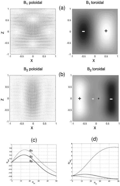
共i兲 The flow rotation acting on B1,yinduces a component B_2,xparallel but opposite to the applied field as shown in Fig.

8共a兲. This starts the expulsion of the transverse B₀ by the axial vorticity of the flow, in the same manner as described in Sec. III.

共ii兲 The action of the axial pumping on B1,y and the

action of the rotation on B1,z both lead to the induction of

poloidal magnetic field lines B2,z in the y Oz plane 关Figs.

8共b兲 and 8共c兲兴. They are generated by the induction current j2

which has a strong component in the direction of the applied field B0, as shown in Fig. 8共d兲. One thus has j2⬀B0 in the

FIG. 8. Transverse applied field,共SD兲 geometry: second order induction. 共a兲, 共b兲 Projection of the second order induced field in the xOz and yOz planes; 共c兲 magnetic field stream lines;共d兲 induced current; 共e兲 net magnetic field up to second order; the stream line is selected to emphasize the ‘‘␣’’-effect mechanism.

2539 Phys. Fluids, Vol. 16, No. 7, July 2004 An iterative study of induction effects

midplane of the flow—note that the currents are confined, so that near the walls of the cylinder they curl to loop inside the flow volume. j2is thus parallel to B0only in the center of the

cell. The proportionality constant is quadratic in Rm and results from helicity of the flow: both the axial and rotational flow components have been needed to produce this second order mechanism. We call this effect an ‘‘␣’’ effect, in anal-ogy with the name introduced in the development of mean-field hydrodynamics by Ra¨dler and Krause.30However, here it is not a result of small scale contributions, but a macro-scopic effect associated with the stretching and twisting of the applied field as originally proposed by Parker.29Adding the first and second order induced fields to the applied one, it

is actually possible to identify field lines that have the very topology proposed by Parker29—Fig. 8共e兲.

B. Evolution with Rm

We first discuss the behavior at low to moderate mag-netic Reynolds numbers, i.e., before field expulsion becomes dominant共Rm⭐5兲. As the applied field has broken the axi-symmetry, we treat induction separately for the xOz and

y Oz planes. We report the variations with Rm of the

mag-netic field computed at three different points in the flow vol-ume. In the y Oz plane, Figs. 9共a兲, 9共b兲, and 9共c兲, the induc-tion is dominated at low Rm by the ‘‘␣’’ mechanism. The x

FIG. 9. Transverse applied field,共SD兲 geometry: local induction vs Rm. Points on the y axis in the right figures, at y⫽0.25, 0.5, 0.75; and on the x axis in the left figures, at x⫽0.25, 0.5, 0.75.

and z components vary quadratically with Rm, while the y

component is mostly linear in Rm. The details of the Bind共Rm) curves depend on the point of measurement. The␣

effect decreases with r: compare the x and z components in Figs. 9共a兲, 9共b兲, and 9共c兲 where measurements are taken at distances 0.25, 0.50, and 0.75 from the rotation axis. In the

xOz plane关cf. Figs. 9共d兲, 9共e兲, and 9共f兲兴 the x component of

the induced field displays a mostly quadratic variation with Rm 共the expulsion effect兲 whereas the other two have a strong linear dependence. Qualitatively, these results are in very good agreement with the measurements made in flows having the same geometry.15,31

As the magnetic Reynolds number is further increased, the expulsion of the applied field from the core of the flow operates. Both the axial and toroidal vorticity components contribute to this expulsion. As a result the ‘‘␣’’-induction process is progressively cutoff from its source and its effi-ciency decreases. This evolution is also in good quantitative agreement with the measurements made in liquid sodium at Reynolds numbers up to 40: compare for example Fig. 5 in Ref. 31 and Fig. 9共b兲 here.

The predominance of expulsion at large Rm corresponds to a two-step negative loop-back mechanism at high orders of iteration. For example, we have observed that at large n, Bn⫹2⯝␥Bn with ␥⫽⫺3.63⫻10⫺2. The value Rm*

⫽1/

冑

conver-gence of the integer series 共the curves in Fig. 9 have been computed using Pade´ approximants兲.

VI. AN ALPHA–OMEGA COOPERATIVE MECHANISM We consider again the共DD兲 flow geometry, i.e., the von Ka´rma´n flow generated by the counter-rotation of the driving disks. In each half of the cylinder the mean flow geometry is very similar to the共SD兲 geometry where it is known that the ‘‘␣’’ effect generates an induced axial field from the applied transverse one. As the sign of the helicity is identical in both half cells, their contributions should add up. We thus expect in the共DD兲 case that when a transverse field 共perpendicular to the cylinder axis兲 is applied, an axial field is induced in a two-step 共quadratic兲 ‘‘␣’’ mechanism. This induced field is distorted by the ␻effect; in this process, a field component

parallel to the initial applied field is generated, in a three-step

共cubic兲 mechanism. This sequence—detailed in Fig. 10—

constitutes a positive induction loop, inducive of dynamo action.

A. The alpha–omega induction process

A transverse external field, B0 parallel to the x axis is

applied to the numerical 共DD兲 flow. Induced fields are com-puted iteratively at Rm⫽1, and shown in Fig. 11. The second order induced field B2—displayed in Fig. 11共a兲—has an

axial component in the y Oz plane. It is maximum in the regions of high helicity (z⫽⫾0.5), in the neighborhood of

y⫽⫾0.5 and has opposite direction on either side of the xOz

plane—as expected from the ‘‘alpha’’ mechanism described in the previous section. Note that, except for some magnetic diffusion, Fig. 11共a兲 is equivalent to twice the induction in Fig. 8共a兲. The third order induced field is shown in Fig. 11共b兲: one observes in the median plane the generation of a strong component of B3 along the x axis (xOz plane兲. It

corresponds to the torsion of the axial component of B2 by

the differential rotation, via the␻effect. One thus obtains an induced field component aligned with the applied field B₀, in agreement with the ‘‘␣’’–␻ picture qualitatively described earlier.

Such a third order induction process can only be ob-served if the magnetic Reynolds number of the flow becomes large enough. Figure 12 shows the development of the in-duced magnetic field as Rm increases, for a point in the median plane. The direct series summation diverges for Rm⬎Rm*⫽8.5 but was extrapolated by Pade´ approximants.

In Fig. 12共a兲 one observes that at low Rm, the x component of Bindis negative and linear: it is due to the compression of

the applied field by the radial flow 共directed towards the rotation axis in the midplane兲. The tendency is reversed at higher Rm, and the x component of Bindbecomes positive for

Rm⬎17.

A similar variation of the induced field in the case of an applied transverse field has been observed experimentally in the von Ka´rma´n sodium共VKS兲 experiment; in fact the evo-lution of B_ind,xin Fig. 12共a兲 is quite similar to that in Fig. 5 of Ref. 19.

FIG. 10. ‘‘Alpha’’–omega dynamo mechanism in the共DD兲 geometry: the applied transverse field 共left兲 gives rise to the axial field displayed the middle figure—the ‘‘␣’’ step; via the⍀ effect, a third order induced field B3is induced, parallel to B0.

2541 Phys. Fluids, Vol. 16, No. 7, July 2004 An iterative study of induction effects

B. An alpha–omega dynamo?

Starting from a initial transverse field, we have thus identified a three-step positive loop-back mechanism. It is tempting to associate this finding with the kinematic dyna-mos observed in von Ka´rma´n flows.11,12 It would provide a concrete mechanism for dynamo action—kinematic simula-tions address only the eventual existence of dynamo instabil-ity for a given flow, but do not explain how self generation is achieved. The knowledge of a dynamo mechanism is essen-tial from the experimental point of view because it yields the possibility to optimize the dynamo cycle and thus lower the critical magnetic Reynolds number. However, the identifica-tion of von Ka´rma´n dynamos with the ‘‘␣’’–␻ process de-scribed here should be made with some care.

Indeed, we have observed in our numerical study that when the iteration is carried to large orders, the dominant contribution comes from the expulsion of the magnetic field from the eddies in the flow. A two-step negative loop-back mechanism sets in. For example, at large n Bn⫹2 is parallel

and opposite to Bn, with ␥⫽⫺1.39⫻10⫺2. This gives a

critical value Rm*⫽1/

冑

ob-served critical value for the convergence of the numerical series.

It does not mean that the ‘‘␣’’–␻mechanism should be ruled out, but rather that it is not efficient enough in the flow geometry considered here to overcome the expulsion effect. To wit, let us return to Fig. 11共c兲: one may observe there that the generation of B3,xoccurs predominantly in the center of

the flow, where differential rotation is strongest. However,

B3,x tends to vanish near z⫽⫾0.5, in the regions of large

vorticity where the ‘‘␣’’ effect is strongest. The coupling be-tween the two effects is thus far from being optimal and it may explain why it does not survive at the large Rm.

The earlier considerations are consistent with the obser-vations that dynamo action in von Ka´rma´n flows is ex-tremely sensitive to the fine details of the flow geometry. For example, the ratio of the intensities of poloidal to toroidal velocity components ( P/T ratio兲 is known to play a funda-mental role. Duddley and James11in their kinematic

simula-FIG. 11. ‘‘␣’’–␻induced fields in the共DD兲 geometry; B0is applied along the x axis. 共a兲 Second order field B2; 共b兲 third order field B3 共the gray arrows serve as an eye-guide兲; 共c兲 three-dimensional view; selected second order and third order magnetic field lines are shown; the contour plot dis-plays B3,x.

FIG. 12. ‘‘Alpha’’–omega induced fields in the共DD兲 geometry; evolution of the induced field Bindwith the magnetic Reynolds number, computed using Pade´ approximants.共a兲 At (x⫽0, y⫽0.5, z⫽0); 共b兲 comparison of the induced x component for various values of the poloidal to toroidal speeds ratio; dashed line:

tions in a spherical geometry have observed that self-generation occurs when P/T⯝0.14, but not when P/T⫽0.1 or P/T⫽0.2. If the toroidal velocity becomes too large, ex-pulsion will surely dominate, but when it is too small the helicity and differential rotation are insufficient for an ‘‘␣’’–␻mechanism to develop. The results shown so far in our numerical study have been obtained for P/T⫽0.8, the optimal value as suggested by kinematic dynamo simulations.12This value also corresponds to the optimal ef-ficiency of the ‘‘␣’’–␻ mechanism, as pointed out in Fig. 12共b兲.

VII. INFLUENCE OF BOUNDARY CONDITIONS

One advantage of our iterative procedure is that various electrical boundary conditions can be considered. This is of importance because in real situations共natural or laboratory兲, the flow of conducting liquid is confined within walls whose electrical conductivity, magnetic permeability, thickness, etc., are important parameters in the induction process. The reason is that the magnetic diffusive length of liquid metals is often comparable to the integral length scale. For example,

it has been shown that a conductive layer at rest surrounding the flow lowers the dynamo threshold in experimental con-figurations as tested in Riga and Karlsruhe.13In this section, we first show that sizeable induction effects can result from the electrical boundary condition 共BC effect兲, giving rise to induced magnetic field contributions which must be added to the bulk effects.

A. BC effect for a transverse applied field

Let us consider the case of the counter-rotating von Ka´rma´n geometry 共DD flow兲, when an external field B₀ is applied perpendicular to the rotation axis, in the x direction. We start with the case of insulating boundary conditions at the flow wall and we will discuss later the generalization to other electrical conditions共note that it is the discontinuity of magnetic diffusivity that matters兲.

Let us first describe the BC effect in a qualitative man-ner. Because of the differential rotation, the B₀field lines are twisted to generate an induced component in the y direction in the median plane—see Figs. 13共a兲 and 13共b兲. Actually, this is the first step in the generation of the ‘‘␣’’ effect described

FIG. 13. Schematics of the BC effect for a transverse applied field B0along the x axis;共a兲 initial field and disks rotation; 共b兲 the radial differential rotation

generates a perpendicular component B1,y; 共c兲 corresponding induced current sheet j1,x; 共d兲 axial B1,BC,z generated at the wall (y⫽⫾R), due to the

discontinuity in the magnetic diffusivity.

2543 Phys. Fluids, Vol. 16, No. 7, July 2004 An iterative study of induction effects

in Sec. V. This field component B1,y is associated with a

current layer j1,x that flows parallel to the applied field, and

in opposite direction in the median plane. As the outside medium is electrically insulating, this current remains within the flow volume and is therefore tangent to the cylindrical vessel on the y axis—see Fig. 13共c兲. At the wall, the discon-tinuity in j1,x creates an axial magnetic field B1,BC,z outside

of the flow volume, cf. Fig. 13共d兲. This field penetrates inside the flow because the diffusion length (R/

冑

component B1,BC,z can also be viewed as a necessity for the

reconnection of the magnetic field lines of B1 at the lateral

walls. We thus observe that this effect cannot exist indepen-dently of bulk induction effects; discontinuities of electrical conductivity alone do not generate an induced field!

The schematic picture described above is supported by the numerical simulation. Figure 14共a兲 shows the induced current in the xOy plane, which lies parallel to the applied field in the middle of the cell. It is therefore tangent to the cylinder walls near y⫽⫾R. At these points the current dis-continuity generates the induced field B1,BC,z as shown in

Fig. 14共b兲. The evolution of this component inside the flow

volume is shown in Fig. 14共c兲: as expected it is maximum at the wall and decreases slowly away from it共its value is only halved at y⫽0.7). The BC effect is essentially linear as can be observed in Fig. 14共d兲 where the evolution of the induced magnetic field with the Reynolds number at point (x⫽0, y

⫽0.5, z⫽0) is reported: the dashed line shows the

contribu-tion of the first order induccontribu-tion alone, while the solid line has been computed summing all orders.

Finally, we should comment upon the symmetries of the field induced by this boundary effect: even symmetry with respect to the xO y plane and odd symmetry with respect to the xOz plane. No linear bulk induction mechanism has the same symmetries. Indeed, in the bulk, the axial field at first order is generated by the radial gradient of the axial flow共a

B0cos␪⳵ruzterm in the induction equation兲, a term which is

odd with respect to the xOy plane. Thus there is no linear bulk effect that can produce a field which is even in symme-try with respect to the xO y plane. However, the quadratic ‘‘␣’’ effect has the same symmetries as the BC effect. In actual experimental situations, both effects will occur simul-taneously; but if the induction is observed to vary mainly linearly with the magnetic Reynolds number one may con-clude that the effect of boundary conditions are dominant over the ‘‘␣’’ effect—as in the VKS measurements.17

We now discuss further some of the properties of this induction effect due to boundary conditions. As noted in Sec. II A, inhomogeneities in the magnetic diffusivity can be

in-FIG. 14. BC effect,共DD兲 geometry: simulations 共experimental flow field兲. 共a兲 First order induced current j1in the xOy at height z⫽0; 共b兲 corresponding magnetic field in the y Oz plane;共c兲 profile of the BC-induced field B1,BC,z(y ) in median plane;共d兲 evolution with the magnetic Reynolds number at (x

cluded in the induction equation 关Eq. 共1兲兴. To lowest order, as we have seen that the BC effect is mostly linear, it can be written as

␭⌬B1⫽⫺“Ã共uÃB0兲⫺关␭兴共S兲␦共S兲共“ÃB1兲⫻n, 共31兲

where S is the surface over which the magnetic diffusivity discontinuity occurs, n the outgoing normal, 关␭兴(S) is the

jump in magnetic diffusivity and ␦(S) a Dirac distribution

null everywhere except on S. This is a closed form in which B1 results both from the bulk and boundary effects. It is

possible to separate these contributions because the boundary effects stem from the bulk induction. First, we isolate the specific induction source term that generates the BC effect and express it in terms of the induced current j1:

I1,BC⫽⫺关␭兴共S兲␦共S兲j1Ãn. 共32兲

This current is mainly generated by the bulk induction, so that to lowest order it verifies the Poisson equation

⌬j1⫽⫺

1

␮0␭ 共

B0"“兲␻, 共33兲

where ␻⫽“Ãu is the flow vorticity and we have assumed that the applied field B0 is homogeneous. Using this

formu-lation one expects the BC effect to be quite sensitive to the precise structure 共vorticity distribution兲 of the flow. It is in-deed the case: the BC effect is weak in the numerical model field used in our study, but very strong in actual experiments.15,18The reason is that experimental flows have a stronger radial vorticity gradient in the vicinity of the cyl-inder lateral walls25 and thus promote a stronger induction

according to Eqs.共31兲–共33兲. This is why in order to enhance the BC effect, the curves in Fig. 14 have been computed using experimental flow profiles.

B. When the external walls are a thin conducting shell

As discussed earlier the source term of the BC effect

关Eq. 共31兲兴 is proportional to the jump in magnetic diffusivity

at the wall. It has opposite effects depending on whether the outside medium has a higher or lower electrical conductivity than the fluid. An interesting situation occurs when the flow walls are made of a shell of material with a higher conduc-tivity, surrounded by an insulating medium. For example, this would be the case for a sodium flow enclosed in a cop-per vessel, surrounded by air.

We consider the case of a von Ka´rma´n flow enclosed in a cylindrical vessel with thickness ep and conductivity ␴p

⫽␨␴—cf. Fig. 15共a兲. Note that in such a geometry, the equa-tion for the electric potential共8兲 must take into account the inhomogeneity of the magnetic diffusivity and thus be re-placed by

⌬␾k⫹1⫺“␭"“␾k⫹1⫽“Ã共uÃBk兲⫺“␭"共uÃBk兲, 共34兲

with the condition (“␾)n⫽0 at the outer insulating wall.

We concentrate on␨⫽1 共the walls have an electrical con-ductivity equal to that of the fluid兲 and ␨⫽4.5 共the ratio of electrical conductivities of copper and liquid sodium兲. In each case the variation of the axial field induced by the BC effect with the thickness of the vessel is shown in Fig. 15共b兲

关at point (x⫽0, y⫽0.5, z⫽0)].

FIG. 15. BC effect,共DD兲 geometry 共experimental flow field兲: influence of the vessel thickness and electrical conductivity. 共a兲 Sketch of the vessel geometry;

共b兲 evolution of the first order BC axial induced field, with the thickness of the vessel 共the dashed and solid lines are only meant as guide to the eye兲; 共c兲 and 共d兲 magnetic field topology in the case of a change of the sign of the discontinuity of the electrical conductivity at the wall 共left:␰⬍1; right␰⬎1兲.

2545 Phys. Fluids, Vol. 16, No. 7, July 2004 An iterative study of induction effects

共1兲 When␨⫽1, the boundary effect tends first to decrease as

the thickness of the vessel is increased, up to a thickness

ep equal to approximately 5% of the radius of the

cylin-der. Then for ep⬎0.05R, the magnitude of the

BC-induced field is roughly constant at a value equal to 60% of its amplitude at ep⫽0 共perfectly insulating outside

medium兲.

共2兲 When␨⫽4.5, the BC-induced field remains at a constant

level for ep⭐0.05R, but then decreases and changes its

sign for ep⬎0.13R. For higher values of ep the induced

field remains negative, as expected from a direct calcu-lation with a full external medium with electrical con-ductivity larger than that of the fluid.

We have already mentioned that the BC effect is associ-ated with the reconnection of the bulk magnetic field B1 on

either side of the median plane. We note here that the change of sign of the induced field corresponds to different recon-nection patterns, as shown in Figs. 15共c兲 and 15共d兲 and also observed in laboratory plasma experiments.32

VIII. CONCLUDING REMARKS

In this paper we have presented a new approach of in-duction in flows of conducting liquids, in which the contri-butions are computed iteratively. Its numerical implementa-tion is simple and gives access to the complete set of electromagnetic variables involved in the induction: electric potential, currents, and magnetic field. Realistic boundary conditions can be considered. This scheme proves to be very convenient to identify how induction mechanisms develop as the magnetic Reynolds number of the flow increases, and how they are related to the topology of the flow field. Inves-tigations of geometries that are relevant to geophysical situ-ations are currently underway. In addition, the method which is at present restricted to stationary flows, could be readily extended for simple time-periodic flows.

From a practical point of view our approach has enabled us a clear identification of important induction mechanisms in von Ka´rma´n flows. When compared to experimental mea-surements, our approach has lead to a very good quantitative agreement, without any adjustable parameter.33 The origin and development of the ‘‘␣’’ and ␻ effects have been de-scribed in detail, as well as their interaction with expulsion which seems to dominate when the magnetic Reynolds num-ber becomes large. We have also pointed out that boundary conditions may be essential in the induction process, particu-larly when the magnetic dissipation length is not small com-pared to the flow integral scale 共as is the case of most natural/experimental situations兲. As an example, we have shown that an external layer of conducting material behaves very differently than an external infinite conducting medium. In regards to the dynamo generation, it is viewed here as a positive loop-back mechanism in the iteration of the induc-tion process. A dynamo is identified if the operator G 共Rm independent兲 has a positive eigenvalue. The neutral mode then has the geometry of the associated eigenvector. As ex-plained, this approach has a firm link with the usual kine-matic dynamo framework. In the case of von Ka´rma´n flows,

we have identified a possible ␣–␻ mechanism, responsible for the self generation observed in kinematic simulations.11,12 However, we have also observed that at the highest orders of iteration, a negative feedback loops sets in, associated with the expulsion of the applied field by the large scale eddies of the flow. It shows that expulsion is the most efficient induc-tion mechanism at large Rm, and that it may mask other processes. In fact, the study of the evolution of the mean induced field in the presence of an externally applied mag-netic field may not allow a direct identification of the dy-namo threshold.

ACKNOWLEDGMENTS

The authors thank all members of the VKS team 共A. Chiffaudel, F. Daviaud, S. Fauve, L. Marie´, F. Pe´tre´lis, F. Ravelet, R. Volk兲 with whom we have had numerous fruitful discussions. They are particularly indebted to F. Ravelet for making his experimental flow fields available. They also ac-knowledge stimulating discussions with P. Frick.

1_{J. Larmor, ‘‘How could a rotating body such as the sun become a magnet,’’} Report of the 87th Meeting of the British Association for the Advancement of Science共John Murray, London, 1919兲, pp. 159–160.

2_{F. J. Lowes and I. Wilkinson, ‘‘Geomagnetic dynamo: A laboratory}

model,’’ Nature共London兲 198, 1158 共1963兲.

3_{R. Steglitz and U. Mu¨ller, ‘‘Experimental demonstration of a}

homoge-neous two-scale dynamo,’’ Phys. Fluids 13, 561共2001兲.

4_{A. Gailitis, O. Lielausis, S. Dement’ev, E. Platacis, A. Cifersons, G.}

Ger-beth, T. Gundrum, F. Stefani, M. Christen, H. Ha¨nel, and G. Will, ‘‘De-tection of a flow induced magnetic field eigenmode in the Riga dynamo facility,’’ Phys. Rev. Lett. 84, 4365共2000兲.

5

G. O. Roberts, ‘‘Dynamo action of fluid motions with two-dimensional periodicity,’’ Philos. Trans. R. Soc. London, Ser. A 271, 411共1972兲.

6_{Yu. B. Ponomarenko, ‘‘On the theory of the hydromagnetic dynamo,’’ J.}

Appl. Mech. Tech. Phys. 14, 775共1973兲.

7

A. Tilgner, ‘‘A kinematic dynamo with a small scale velocity field,’’ Phys. Lett. A 226, 75共1997兲.

8_{A. Gailitis, ‘‘Project of a liquid sodium MHD dynamo experiment,’’}

Mag-netohydrodynamics共N.Y.兲 1, 63 共1996兲.

9_{See, for example, L. Marie´, F. Pe´tre´lis, M. Bourgoin, J. Burguete, A.}

Chiffaudel, F. Daviaud, S. Fauve, P. Odier, and J.-F. Pinton, ‘‘Open ques-tions about homogeneous fluid dynamos: The VKS experiment,’’ Magne-tohydrodynamics 38, 163 共2002兲; W. L. Shew, D. R. Sisan, and D. P. Lathrop, ‘‘Mechanically forced and thermally driven flows in liquid so-dium,’’ ibid. 38, 121共2002兲, and references therein.

10

H. K. Moffatt, Magnetic Field Generation in Electrically Conducting

Flu-ids共Cambridge University Press, Cambridge, 1978兲.

11_{N. L. Dudley and R. W. James, ‘‘Time-dependent kinematic dynamos with}

stationary flows,’’ Proc. R. Soc. London, Ser. A 425, 407共1989兲.

12

L. Marie´, J. Burguete, F. Daviaud, and J. Le´orat, ‘‘Numerical study of homogeneous dynamo based on experimental von Ka´rma´n type flows,’’ Eur. Phys. J. B 33, 469共2003兲.

13_{R. Avalos-Zuniga, F. Plunian, and A. Gailitis, ‘‘Influence of}

electromag-netic boundary conditions onto the onset of dynamo action in laboratory experiments,’’ Phys. Rev. E 68, 066307共2003兲.

14_{P. Odier, J.-F. Pinton, and S. Fauve, ‘‘Advection of a magnetic field by a}

turbulent swirling flow,’’ Phys. Rev. E 58, 7397共1998兲.

15_{M. Bourgoin, R. Volk, P. Frick, S. Kripechenko, P. Odier, and J.-F. Pinton,}

‘‘Induction mechanisms in a von Ka´rma´n swirling flow of liquid gallium,’’ Magnetohydrodynamics 40, 13共2004兲.

16_{N. L. Peffley, A. B. Cawthrone, and D. P. Lathrop, ‘‘Toward a}

self-generating magnetic dynamo: The role of turbulence,’’ Phys. Rev. E 61, 5287共2000兲.

17

L. Marie´, J. Burguete, A. Chiffaudel, F. Daviaud, E. Ericher, C. Gasquet, F. Pe´tre´lis, S. Fauve, M. Bourgoin, M. Moulin, P. Odier, J.-F. Pinton, A. Guigon, J.-B. Luciani, F. Namer, and J. Le´orat, ‘‘MHD in von Ka´rma´n swirling flows,’’ in Dynamo and Dynamics: A Mathematical Challenge,