HAL Id: hal-00952233
https://hal.archives-ouvertes.fr/hal-00952233
Submitted on 26 Feb 2014
HAL is a multi-disciplinary open access
archive for the deposit and dissemination of sci-entific research documents, whether they are pub-lished or not. The documents may come from teaching and research institutions in France or abroad, or from public or private research centers.
L’archive ouverte pluridisciplinaire HAL, est destinée au dépôt et à la diffusion de documents scientifiques de niveau recherche, publiés ou non, émanant des établissements d’enseignement et de recherche français ou étrangers, des laboratoires publics ou privés.
PICARD
Abdanour Irbah, Mustapha Meftah, Alain Hauchecorne, Djelloul Djafer,
Thierry Corbard, Maxime Bocquier, Momar Cissé
To cite this version:
Abdanour Irbah, Mustapha Meftah, Alain Hauchecorne, Djelloul Djafer, Thierry Corbard, et al.. New space value of the solar oblateness obtained with PICARD. The Astrophysical Journal, American Astronomical Society, 2014, 785 (2), pp.89. �10.1088/0004-637X/785/2/89�. �hal-00952233�
Abdanour Irbah, Mustapha Meftah, Alain Hauchecorne
Laboratoire Atmosph`eres, Milieux, Observations Spatiales (LATMOS), CNRS : UMR 8190 - Universit´e Paris VI - Pierre et Marie Curie - Universit´e de Versailles
Saint-Quentin-en-Yvelines - INSU, 78280, Guyancourt, France
Djelloul Djafer
Unit´e de Recherche Appliqu´ee en Energies Renouvelables, URAER, Centre de D´eveloppement des Energies Renouvelables, CDER, 47133, Gharda¨ıa, Algeria
Thierry Corbard
Laboratoire Lagrange, UMR7293, Universit´e de Nice Sophia-Antipolis, CNRS, Observatoire de la Cˆote d’Azur, Bd. de l’Observatoire, 06304 Nice, France
Maxime Bocquier
and
E. Momar Cisse
Laboratoire Atmosph`eres, Milieux, Observations Spatiales (LATMOS), CNRS : UMR 8190 - Universit´e Paris VI - Pierre et Marie Curie - Universit´e de Versailles
Saint-Quentin-en-Yvelines - INSU, 78280, Guyancourt, France
ABSTRACT
The PICARD spacecraft was launched on June 15, 2010 with one of its sci-entific objectives the study of the geometry of the Sun. The measure of the solar oblateness remains difficult because images are affected by optical distortions. Rolling the satellite as performed in previous space missions, allows determi-nation of the telescope contribution by assuming the geometry of the Sun is constant during the observations. This supposes that the telescope optical re-sponse is time-invariant during the roll operations. It is not the case for PICARD since an orbital signature is clearly observed in the solar radius computed from its images. We take into account this effect and provide the new space value of the solar oblateness obtained from PICARD images recorded in the solar continuum at 535.7 nm in July 4-5, 2011. We obtain 8.4 ± 0.5 mas for the equator-pole radius difference, which corresponds to an absolute radius difference of 6.1 kilometers. It is in good agreement with the mean value of all solar oblate-ness measurements obtained during the two last decades from ground, balloons and space. It is also consistent with values determined from models using helioseismology data.
1. Introduction
The measurement of the solar diameter has been debated question since the possibility of an oblate Sun was first asked by Newcomb in 1865 when he wondered why Newtonian gravitational theory could not correctly predict the anomalous advance of Mercury perihelion (Newcomb 1865). He suggested that an oblateness of 500 milli-arcseconds (mas) would explain such a phenomena. If it is admitted today that Einstein’s theory of General Relativity well explains the advance anomalous of the Mercury perihelion, it remains that a good estimate of the solar oblateness is of great importance for this theory i.e. the gravitational moments of the Sun is still relevant for the Mercury perihelion (Chapman 2008). Moreover, they depend on the rotation of the inner layers of the Sun, which is estimated by mean of others techniques such as helioseismology (Mecheri et al. 2004). Constraints on solar oblateness have been developed from other studies in particular on the rotation of the solar core (Chapman 2008). Many attempts to measure the solar oblateness have been made since the first one by Auwers (1891). Several decades later in 1966, new measurements started at Princeton on Wilson Mount in 1983, 1984 and 1985 (Dicke et al. 1987). The obtained values of an equator-pole radius difference ranged from 5.6 to 41.9 mas. A measurement made during this period should be mentioned. It was obtained with the SCLERA (Santa Catalina Laboratory for Experimental Relativity by Astrometry) telescope under excellent weather conditions leading to 9.2 ± 6.3 mas (Hill & Stebbins 1975), which is consistent with the most recent experimental values. Let us focus on the measurements obtained with the Pic du Midi heliometer, which operated from 1996 to 2008 (see Rozelot and Lefebvre (2003) for a description) and the Solar Disk Sextant (SDS) campaigns from a stratospheric balloon (1992-1996). The SDS balloons flew at 340 km in New-Mexico and used a mechanically and optically stable Beam Splitting Wedge (BSW) in front of a telescope to make images of the Sun. The radius was measured in the 590-670 nm band (Egidi et al. 2005). For the oblateness analysis, the telescope rotates
around its optical axis for several cycles. The angular radius is band-pass filtered and fitted by a sine function which maximum and minimum provide the oblateness. The results obtained with these two instruments are plotted in Figure 7, and will be discussed in section 4.
When measurements are made from ground-based facilities, the results suffer from atmo-spheric blurring and incoherent distortion noise on the limb. In space, those distortions are mainly due to the spacecraft pointing and optical distortion which are coherent across the image, or temporally slowly varying, in a way that they can be removed more easily. The space measurements of the solar oblateness were made by three distinct instruments: the Michelson Doppler Imager (MDI) from the SOlar and Heliospheric Observatory (SOHO) satellite (Scherrer et al. 1995), the Reuven Ramaty High Energy Solar Spectroscopic Imager (RHESSI) spacecraft which provides images of high-energy radiation solar sources (Fivian et al. 2008) and the Helioseismic and Magnetic Imager (HMI) from NASA’s Solar Dynamics Observer (SDO) (Kuhn et al. 2012). (i) The SOHO spacecraft was launched on December 2, 1995. The analysis of the Solar shape were made in 1997 and in 2001 with a special roll procedure to remove instrumental influences. Two values are provided by the MDI instrument from the Limb Darkening Function (LDF) analysis : 8.7 ± 2.8 mas (1997) and 18.9 ± 1.9 mas (2001) (Emilio et al. 2007). Still, those values suffer from the defocus and blurring of the instrument optics. (ii) RHESSI is a solar observatory whose Sun images are provided by the Solar Aspect Sensor, a simple lens (4 cm diameter) imager working with a 12 nm band-pass at 670 nm. The oblateness is there determined with the asymmetric quadrupole term of the Fourier components of the limb position. Its value is 10.77 ± 0.44 mas obtained during the period June 29 to September 24, 2004 from a data set selected to avoid active regions. The solar magnetic activity at the limb is advanced by the authors to explain an excess of this previous value. The equator-pole radius difference is reduced to 8.01 ± 0.14 mas corresponding to a nonmagnetic Sun obtained
when a threshold is applied in the EUV data (Fivian et al. 2008). Chapman affirmed then that this result eliminated the possibility of a rapidly rotating core (Chapman 2008). (iii) SDO was launched on February 11, 2010. HMI observes the full solar disk at 617.3 nm with a resolution of 1 arc-second. The spacecraft does roll calibrations twice a year allowing the instrument to calculate the solar oblateness at the same time. A mean value of 7.20 ± 0.49 mas for the equator-pole radius difference was calculated from 6 roll-sequences after evaluating the LDF, correcting it from brightness and fitting the results with a quadrupole and fourth-order Legendre polynomials (Kuhn et al. 2012). The period to calculate the mean value extends from 2010 to 2012. The HMI measurement is significantly lower than the others space values.
It is in this context of the oblateness measurement that the PICARD value is ex-pected (Chapman 2008; Mecheri et al. 2004) from observations made by its onboard telescope, the Solar Diameter Imager and Surface Mapper (SODISM) (Meftah et al. 2014a). It was observing at the same period as HMI. We present in this paper a new space value of the solar oblateness obtained in July 4-5, 2011 with SODISM in the solar continuum at 535.7 nm. We begin first by giving an overview of the PICARD mission and its observations. We then present the method we use to process the solar images recorded with SODISM. We finish by giving the results we obtain and discuss them.
2. The PICARD mission and its observations
First, we give a brief description of the PICARD mission and its telescope SODISM. Then, we present the distortion mode and the observations, which indicates that the low spacecraft orbit required the development of additional analysis techniques.
2.1. The PICARD telescope
The PICARD solar mission was launched on June 15, 2010 and will continue to observe until early 2014. Its main objectives are the measurements of the diameter and the asphericity of the Sun at several wavelengths (215, 393.37, 535.7, 607.1 and 782.2 nm), the limb shape at the same wavelengths, the differential rotation, the Total Solar Irradiance (TSI), the Spectral Solar Irradiance (SSI) in UV, visible and IR, and to get images for helioseismologic studies to probe the inner Sun. The PICARD mission operates during the rising phase of the solar cycle 24, allowing us to study the variation of these quantities with the solar activity. The satellite is in a Sun synchronous Orbit with an ascending node at 06h00, an orbit inclination of 98 degrees, an altitude of 730 km and a period of about 100 minutes. Annual eclipses exist in such orbits, but they last for 20 minutes maximum (for instance in December). The total PICARD payload weight is about 125 kg. It includes absolute radiometers and photometers for the TSI and SSI measurements and SODISM, an imaging telescope developed to measure the diameter, the limb shape and the asphericity of the Sun. A detailed description of the PICARD telescope may be found in Meftah et al. (2014a). We recall here some of its main properties. SODISM images the whole solar disk on a CCD (Charge-Coupled Device) sensor. A window is set in front of the telescope to limit the solar energy to 5% of the total solar irradiance. Wavelengths are selected by interference filters on 2 wheels. Wavelength domains are chosen free of Fraunhofer lines (535.7, 607.1 and 782.2 nm). Active regions are detected in the 215 nm domain and the CaII (393.37 nm) line. Helioseismologic observations are performed at 535.7 nm (Corbard et al. 2013). The spacecraft pointing is stabilized to better than 36 arc-seconds. The telescope primary mirror stabilizes the solar image within 0.2 arc-second, using a proper piezo-electric system. An internal calibration system is used to determine scale factor variations induced by instrument deformations, which result from temperature fluctuations in orbit or others causes (Irbah et al. 2012; Assus et al. 2008). The diameter
measurements are referred to star angular distances by rotating the spacecraft towards some doublet stars several times a year. The instrument stability is ensured by the use of stable materials (Zerodur for mirrors, Carbon-Carbon and Invar for structure). The whole instrument temperature is stabilized within 1oC, the CCD around −7oC within 0.2oC.
2.2. The PICARD distortion mode and a preliminary analysis
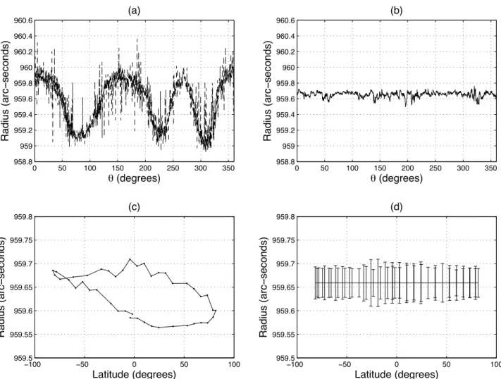
PICARD has several observation modes. The most important are the nominal, the distortion and the stellar modes. In this last mode, the telescope takes star images useful for the scale factor estimation. In the two first ones, the PICARD telescope records full and limb images of the Sun at all the wavelengths already mentioned. Full resolution solar images are 2048x2048 pixels size. The pixel size was estimated in space using the Venus transit, which occurred in June, 2012. It is equal to 1.064 arc-seconds (Meftah et al. 2014b). Limb images corresponding to 22 or 40 pixels wide limbs (Irbah et al. 2010) are obtained by masking the solar image to take only the pixels where the limb is imaged on the camera. The distortion mode or roll procedure was especially defined to measure the solar asphericity. The Figure 1(a) shows the mean azimuthal variations of the solar radius obtained from the limb image series recorded at 535.7 nm during the roll procedure of July 4-5, 2011. Angular variations of about one arc-second are clearly visible. They are essentially due to the instrument optical distortion. Special methods are then needed to estimate the solar oblateness. A similar roll procedure used for MDI on the spacecraft SOHO (Emilio et al. 2007) and later for HMI on the SDO spacecraft (Kuhn et al. 2012) was deployed for PICARD. The satellite is rotated around the SODISM line of sight by step of 30o. The solar image rotates in the focal plane
relative to the camera axis, which defines the reference frame for the calculations. The solar oblateness is then computed considering the polar and equatorial radii in images that
are collinear (see Figure 2). This is possible by selecting the appropriate images recorded at the different satellite rotation positions. We have here a differential measurement that overcome optical effects. Solar images series are taken during more than one and a half orbit in each angular position of the satellite during the roll procedure. The total time needed for one distortion mode is about 1.6 days. Thus, different pairs of radii such as RP and RE
in Figure 2, are separated by more than one day. The optical system has to remain time invariant during all this period. The Figure 1(b) plots the temporal variations of the mean solar radius extracted from the same limb image series as used before. Temporal variations of more than 0.1 arc-seconds are clearly observed on the radius suggesting that the optical system evolves in its environment. This is also well observed if we plot the mean solar radius versus the latitude when the satellite is in the nominal mode (rotation = 0o) and
rotated by 90o (see Figure 3). This preliminary analysis shows that the PICARD satellite is
affected by Earth atmospheric radiations due to its low orbit (Irbah et al. 2012). We have to be aware of these facts to calculate the solar oblateness.
3. The processing method for the PICARD image analysis
The solar radius versus the azimuthal angle in a polar coordinates system may be expressed as:
r(θ) = ˆRm+ dR(θ)
ˆ
Rm =< r(θ) >Θ=2π is the mean solar radius when the Sun is considered as a sphere and
dR(θ) its radius variation. < . >Θ denotes the average operation carried out on the angular
interval Θ.
The solar radius Rm(θ, t) computed from a PICARD image at t is expressed as:
I(θ) is the angular optical distortion of the PICARD telescope. A(t) introduces the time variation of the mean solar radius due to thermal fluctuations of the PICARD telescope on its orbit. It is given by:
A(t) = 1 + αΨ(2πt
P ) (2)
where α << 1 is the fluctuation amplitude reflecting the radius variations. Ψ(.) is a periodic function with P the period of the satellite (about 100 minutes).
We compute dR(θ) by correcting the radius Rm(θ, t) from I(θ) and A(t). The data used
are image series recorded at several spacecraft roll orientations by the SODISM instrument operating in distortion mode. The solar images rotates in the focal plane relative to the camera axis which is taken as the reference frame (see section 2.2). The optical distortion remains however the same if we consider the Sun as a sphere. Equation 1 becomes in this case:
Rm(θ − k π 6, t) =! ˆRm+ dR(θ − k π 6) " ×I(θ)×A(t) (3)
where k is the rotation number between 0 and 12. The upper value M brings back the satellite to the nominal mode.
We start with a time average of the solar radius computed from the whole N images in the distortion mode data-set:
# $ Rm(θ − kπ 6, tj) % j=1,N|k=1,M & T = I(θ)#A(tj)j=1,N$ ˆRm+ dR(θ − k π 6) % k=1,M & T = I(θ)! ˆRm+ # A(tj)j=1,N $ dR(θ − kπ 6) % k=1,M & T "
where tj is the date of the image j and #x(t)$T stands for the time average of x(t) over
interval T = tN − t1.
We can deduce I(θ) from this Equation:
I(θ) = # 'Rm(θ − k π 6, tj) ( j=1,N|k=1,M & T ˆ Rm since #A(tj)j=1,N $ dR(θ − kπ 6) % k=1,M & T ≈ 0 (4)
Equation 4 gives a first estimate of I(θ) = I1(θ) where ˆRm is a time and angular mean
computed over all the radius from the distortion mode data-set. Then, we use I1(θ) to
correct the solar radius series from optical distortion:
$ Rm1(θ − k π 6, tj) % j=1,N|k=1,M = 'Rm(θ − k π 6, tj) ( j=1,N|k=1,M I1(θ) = A(tj)j=1,N$ ˆRm+ dR(θ − k π 6) % k=1,M
We compute the angular mean of Rm1(θ, t):
# $ Rm(θ − k π 6, tj) % j=1,N|k=1,M & Θ=2π = #A(tj)j=1,N$ ˆRm+ dR(θ − k π 6) % k=1,M & Θ=2π = A(tj)j=1,NRˆm+ A(tj)j=1,N # $ dR(θ − kπ 6) % k=1,M & Θ=2π
A(t) is then deduced from this Equation:
A(tj)j=1,N = # 'Rm1(θ − k π 6, tj) ( j=1,N|k=1,M & Θ=2π ˆ Rm since # $dR(θ − kπ 6) % k=1,M & Θ=2π ≈ 0 (5)
In this Equation, ˆRm is computed as before: time and angular mean of the whole radius series. Equation 5 gives then the first estimate of A(t) = A1(t) that we use to correct the
radius from time variations:
$ Rm2(θ − k π 6, tj) % j=1,N|k=1,M = 'Rm1(θ − k π 6, tj) ( j=1,N|k=1,M A1(tj)j=1,N
This is the first step of an iterative process beginning from Equation 3 applied to Rm2(θ, t)
to correct the solar radius series from residual contributions of I(θ) and A(t). This process ends when Ip(θ) ≈ 1 and Ap(t) ≈ 1(α ≈ 0) (iteration p), leading to:
$ dR(θ − kπ 6) % k=1,M = # 'Rmp(θ − k π 6, tj) ( j=1,N|k=1,M & Θ=2π Ip(θ) × A1(tj)j=1,N − ˆRm (6)
The solar shape dR(θ) is then deduced from #'dR(θ − kπ
6)
(
k=1,M
&
T, which is shifted to
4. Results and discussion
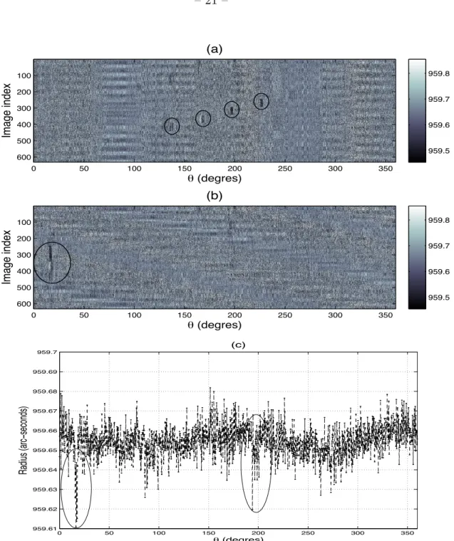
We estimate the oblateness of the Sun in the solar continuum at 535.7 nm using the method described in Section 3. We consider the solar image series taken during the distortion mode on July 4-5, 2011. It is composed of 80 limb images recorded every 2 minutes at each satellite rotation leading to a total number of 1040 images. At each rotation position, only images taken over a single satellite orbit are used in the calculations in order to satisfy Equation 2. The roll procedure lasted about 1.6 days (see section 2.2). Figure 4(a) plots the azimuthal variations of the radius extracted from one image of the data set, and Figure 4(b) the same radius corrected from the optical distortion with our processing method. The one arc-second peak-to-peak value we had in the azimuthal radius variations is lowered to about 30 mas where the solar oblateness signal is in the residual fluctuations. Figures 4(c) and 4(d) plot respectively the latitude dependence of the radius before (see section 2.2) and after corrections. There is no more latitude dependency after applying the processing method. The error bars in the Figure are the standard deviation of the radius values for the different satellite latitudes. We compute dR(θ) at the end of the whole process to obtain the solar oblateness (see section 3). Azimuthal radius variations extracted from all the image series are represented in Figure 5(a) and (b). They are coded in a gray-scale false color where each line is the azimuthal solar radius obtained from one image. Some solar structures shown inside the circles in the Figure affect the radius at several azimuthal angles. They are moving in an oblique direction as the satellite is rotated (see Figure 5(a)). The vertical structures are clearly optical signatures since they remain fixed. Figure 5(b) shows all azimuthal solar radius in the same reference frame i.e. the West Equator is the origin of the azimuthal angles for all lines. We notice that the solar structures surrounded by a circle in the Figure, are now spread along the same vertical direction since they are quasi fixed on the Sun surface having their temporal life. The Solar shape is then obtained taking the radius
median value for each azimuthal angle (see Figure 5(c)). The affected radius by the structures on the Sun surface are shown in the surrounded regions. Figure 6(a) plots the raw solar shape obtained by masking out the active regions. The angular sampling is 0.1o.
We express the solar shape as a linear combination of low order Legendre polynomials Pk(cos(θ)): r(θ) = ˆRm ! 1 + ) k=2,4 ckPk(cos(θ)) " (7)
where θ is the azimuthal angle. k = 2 and k = 4 leads respectively to the quadrupole and the octopole or hexapole distortion terms.
Equation 7 allows to calculate the oblateness: RE− RP ˆ Rm = − 3 2c2 − 5 8c4
Figure 6(b) shows the solar shape obtained after some filtering as well as the Legendre polynomial fit. The filtering consists in a simple data selection by thresholding the residues of a first cosine fit then applying a new angular sampling of 0.3o. The equator-pole
radius difference is found equal to 8.4 mas with an uncertainty of 0.5 mas corresponding to 95% confidence bounds of the fitted parameters. This also corresponds to the absolute radius difference of (6.1 ± 0.4) kilometers and to the solar oblateness coefficients c2 = (−5.71 ± 0.36) × 10−6 and c4 = (−0.36 ± 0.43) × 10−6. When we only correct
for the optical distortion, the equator-pole radius difference is 7.3 mas i.e. 5.3 kilometers for the absolute radius difference with the same uncertainty. This lower value is explained by the temporal variations of the distortion, which have different amplitudes at each satellite position (see Figure 1(b)). They introduce incoherent displacements of the solar limb at the different azimuthal angles leading to a degradation of the final solar shape as shown in Figure 5(c). A lower solar oblateness is then obtained with the degraded solar shape signal
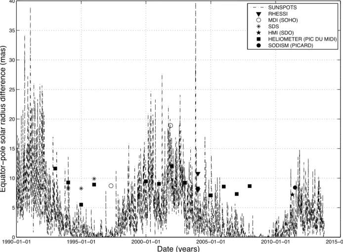
when we fit by polynomial functions. The solar shape is better estimated when we bring the temporal corrections to compensate from incoherent displacements of the solar limb positions. The residual noise due to the corrections and the edge detection leads to the 0.5 mas uncertainty due to the polynomial fit. Let us compare our solar oblateness result with the values previously calculated in the last two decades since there was too many disparities in data before. We consider some instruments operating in different environments during this period. The first one is the Pic du Midi heliometer, a ground-based instrument that provided a long-time series (R¨osch & Rozelot 1996; Rozelot & Bois 1997; Rozelot and Lefebvre 2003; Rozelot & Damiani 2009). The second is the Solar Disk Sextant on balloons, since it is an airborne instrument providing values between ground and space (Sofia, Heaps & Twing 1994; Lydon & Sofia 1996; Egidi et al. 2005). The latter are all space-based instruments from which the solar oblateness measurement was made (Kuhn et al. 1998; Emilio et al. 2007; Fivian et al. 2008; Kuhn et al. 2012). Figure 7 plots the equator-pole radius difference measured during these two last decades. The mean value computed over the considered period is also plotted in solid line as well as the PICARD oblateness value with its error bar. Our result is found very close to the mean value equal to 8.6 mas corresponding to an absolute radius difference of 6.2 kilometers. If we compare with space measurements considering only the c2 oblateness term since our c4 value is less well estimated, we see clearly that
we have a result close to the values obtain with MDI in March 1997 (Kuhn et al. 1998) at 676.8 nm and RHESSI from June to September 2004 at 670 nm (Fivian et al. 2008) even if our images are recorded at 535.7 nm. In addition, these measurements were made during minimum or medium solar activity (rising and falling phase of the solar cycle) (see Figure 8). It is however slightly greater than the mean value obtained with HMI on the SDO spacecraft during the period 2010 to 2012. (Kuhn et al. 2012). Finally, our result is compatible with both the observed surface rotation rate and the values of c2
based on internal rotation profiles estimated from helioseismology (Mecheri et al. (2004)). It is also consistent with the c2 value (c2 = −5.87 × 10⁻⁶) given by Armstrong &
Kuhn (1999) obtained from helioseismology data too .
5. Conclusion
A new space value of the solar oblateness is provided by the PICARD mission. It has been obtained from the images recorded in the solar continuum at 535.7 nm. The roll procedure of PICARD was deployed in July 4-5, 2011 allowing distortion corrections in the calculation of the solar oblateness. Some radiation incoming from the Earth affect however the observations since the PICARD satellite is on a low orbit. A method taking into account these effects has been developed and presented in this paper. It allows to process correctly the PICARD images and consequently estimate the solar oblateness. We obtain 8.4 mas for the equator-pole solar radius difference with an uncertainty estimated to 0.5 mas. This value corresponds to the absolute radius difference of (6.1 ± 0.4) kilometers. It is coherent with the mean value obtained from all oblateness measurements made during the two last decades with the Pic du Midi heliometer, with SDS on balloon flights and from space. The PICARD oblateness is also consistent with the values obtained from models that use helioseismology data.
This work has been supported by the French National Centre for Sciences (CNRS) and the French space Agency (CNES).
REFERENCES
Armstrong, J. & Kuhn, J. R., 1999, ApJ, 525, 1, 533
Assus, P., Irbah, A., Bourget, P., Corbard, T. & the PICARD team, 2008, Astron. Nachr., 329, 5, 517
Auwers, A., 1891, Astron. Nachr., 128, 361
Chapman, R., 2008, Science, 322, 535
Corbard, T., Salabert, D., Boumier, P., Appourchaux, T., Hauchecorne, A. et al, 2013, Journal of Physics: Conference Series, 440, 012025
Dicke, R. H., Kuhn, J. R. & Libbrecht, K. G., 1987, ApJ, 318, 451
Egidi, R., Caccin, B., Sofia, S., Heaps, W., Hoegy et al, 2006, Sol. Phys., 235, 410
Emilio, M., Bush, R.I., Kuhn, J., Sherrer, P., 2007, ApJ, 660, L161
Fivian, M., Hudson, H., Lin, R., Zahid, H., 2008, Science, 322, 560
Hill, H.A. & Stebbins, R.T., 1975, ApJ, 200, 471
Irbah, A., Dufour, C., Meftah, M., Meissonnier, M, Thuillier, G. et al., 2010, Astron. Nachr., 331, 9-10, 59
Irbah, A., Meftah, M., Hauchecorne, A., Cisse, M & Rouze, M., 2012, Proceedings SPIE 8442, Space Telescopes and Instrumentation 2012: Optical, Infrared, and Millimeter Wave, Amsterdam : Netherlands
Kuhn, J.R., Bush, R., Emilio, E., Scholl, I.F., 2012, Science 337, 1638
Lydon, T.J., Sofia, S., 1996, Physical Review letters, 76, 177
Mecheri, R., Abdelatif, T., Irbah, A., Provost, J., Berthomieu, G., 2004, Sol. Phys., 222, 2, 191
Meftah, M., Hochedez, J.F., Irbah, A., Hochedez, J.F. & Corbah, C., 2014a, Sol. Phys., 289, Issue 3, 1043
Meftah, M., Hauchecorne, A., Crepel,M., Irbah, A., Hauchecorne, A. et al., 2014b, Sol. Phys., 289, Issue 1, 1
Newcomb, S., 1865, Constants of astronomy, US GPO, Washington, DC, 111
R¨osch, J., Rozelot, J.P., 1996, C. R. Acd. Sci., Paris, s´erie II, 322, 637
Rozelot, J.P., Bois, E., 1997, New results concerning the solar oblateness and consequences on the solar interior, In: Balasubramaniam, K.S., Rabin, D.M. (Eds.), 18th NSO Workshop, Sacramento Peak, USA, Conference of the Pacific Astronomical Society, 140, 75
Rozelot, J.P., Lefebvre, S., 2003, The figure of the Sun, astrophysical consequences, In: The Sun’s surface and subsurface, Investigating shape and irradiance, Lecture notes in Physics, 599, 4
Rozelot, J.P., Daminani, C., 2009, ApJ, 703, 1791
Scherrer, P. H., Bogart, R. S., Bush, R. I., Hoeksema, J. T., Kosovichev, A. G et al., 1995, Sol. Phys., 162, Issue 1-2, 129
Sofia, S., Heaps, W., Twigg, L.W., 1994, ApJ, 427, 1048
0 50 100 150 200 250 300 350 958.8 959 959.2 959.4 959.6 959.8 960 960.2 960.4 960.6 θ (degrees) Radius (arc − seconds) (a)
Jul−04−2011 04:48 Jul−04−2011 14:24 Jul−05−2011 00:00 Jul−05−2011 09:36 Jul−05−2011 19:12 959.46 959.48 959.5 959.52 959.54 959.56 959.58 959.6 959.62 959.64 Date Radius (arc − seconds) (b)
Fig. 1.— Azimuthal variation of the mean solar radius obtained from the images recorded at 535.7 nm during the distortion mode of July 4-5, 2011 (a). The zero is the solar West Equator. The temporal variations of the mean radius extracted from each image is shown in (b) : fluctuations with the satellite orbit are clearly observed.
−100 −80 −60 −40 −20 0 20 40 60 80 100 959.56 959.58 959.6 959.62 959.64 959.66 959.68 959.7 959.72 Latitude (degrees) Radius (arc − seconds) (a) −100 −80 −60 −40 −20 0 20 40 60 80 100 959.5 959.55 959.6 959.65 959.7 959.75 Latitude (degrees) Radius (arc − seconds) (b)
Fig. 3.— PICARD distortion mode of July 4-5, 2011 : mean solar radius at 535.7 nm versus the latitude for a satellite rotation of 0o (top) and 90o (bottom).
0 50 100 150 200 250 300 350 958.8 959 959.2 959.4 959.6 959.8 960 960.2 960.4 960.6 θ (degrees) Radius (arc − seconds) (a) 0 50 100 150 200 250 300 350 958.8 959 959.2 959.4 959.6 959.8 960 960.2 960.4 960.6 θ (degrees) Radius (arc − seconds) (b) −100 −50 0 50 100 959.5 959.55 959.6 959.65 959.7 959.75 959.8 Latitude (degrees) Radius (arc − seconds) (c) −100 −50 0 50 100 959.5 959.55 959.6 959.65 959.7 959.75 959.8 Latitude (degrees) Radius (arc − seconds) (d)
Fig. 4.— Correction of the solar edge from the optical distortion with our processing method (the zero is the solar West Equator): before (a) and after (b) corrections. Same results for the radius dependance with the satellite latitude when the satellite rotation is 0o: before (c)
θ (degres) Image index (a) 0 50 100 150 200 250 300 350 100 200 300 400 500 600 θ (degres) Image index (b) 0 50 100 150 200 250 300 350 100 200 300 400 500 600 959.5 959.6 959.7 959.8 959.5 959.6 959.7 959.8 0 50 100 150 200 250 300 350 959.61 959.62 959.63 959.64 959.65 959.66 959.67 959.68 959.69 959.7 θ (degres) Radius (arc −seconds) (c)
Fig. 5.— Azimuthal variation of the solar radius extracted from the distortion mode of July 4-5, 2011. (a) : Each line is coded in a gray scale false color and represents the solar radius obtained from one image of the series. Some solar structures shown inside the circles affect the radius estimation at several azimuthal angles. They are moving as the solar axis when the satellite is rotated. The image vertical structures are clearly optical signature since they are fixed. (b) : All solar radius in the same reference axis i.e. the West Equator is the origin of the azimuthal angles for all lines. We notice that the solar structures are now on the same vertical (inside the circle) since they are fixed on the Sun surface and have their temporal life. (c) Solar shape affected by the structures on the Sun surface (surrounded regions).
0 50 100 150 200 250 300 350 959.61 959.62 959.63 959.64 959.65 959.66 959.67 959.68 959.69 959.7 θ (degres) Radius (arc − seconds) (a) 0 50 100 150 200 250 300 350 959.63 959.64 959.65 959.66 959.67 959.68 θ (degres) Radius (arc − seconds) (b)
Fig. 6.— (a) is the raw result of the solar shape obtained from the PICARD distortion mode of July 4-5, 2011 excluding the actives regions. (b) is the filtered solar shape with its fitted curve. The Legendre polynomial fit leads to a solar oblateness of 8.4 mas.
19902 1995 2000 2005 2010 2015 4 6 8 10 12 14 16 18 20 22 Date (years) Equator −
pole solar radius difference (mas)
Mean value of solar radius difference RHESSI MDI (SOHO) SDS HMI (SDO)
HELIOMETER (PIC DU MIDI) SODISM (PICARD)
Fig. 7.— The equator-pole solar radius difference measured since 1992 from a ground-based instrument (heliometer at the Pic du Midi in France), balloon and space. The mean value of all measurements is also represented as well as the value obtained with PICARD. The HMI (SDO) value is the mean of all measurements obtained during the period 2010-2012 (Kuhn et al. 2010-2012)
1990−01−010 1995−01−01 2000−01−01 2005−01−01 2010−01−01 2015−01−01 5 10 15 20 25 30 35 40 Date (years) Equator −
pole solar radius difference (mas)
SUNSPOTS RHESSI MDI (SOHO) SDS HMI (SDO)
HELIOMETER (PIC DU MIDI) SODISM (PICARD)
Fig. 8.— The measurements of the equator-pole radius difference considered in this study and the solar activity since 1990 (cycle 22) up today (current cycle 24) (the sunspot number giving the activity is divided by 200 for the needs of the representation. The Sunspot data comes from http://solarscience.msfc.nasa.gov)